Inertial Navigation Static Calibration
Slawomir Niespodziany
Abstract—Inertial navigation is a device, which estimates its position, based on sensing external conditions (such as acceleration or angular velocity). It is widely used in variuos applications. Its presence in a drone vehicle for example, allows flight stabilization, by position estimation and feedback-based regulation algorithm execution. A smartphone makes a use of inertial navigation by detecting movement and flipping screen orientation. It is a ubiquitous part of many devices of everyday use, but before using filters and algorithms allowing to calculate the position, a calibration must first be applied to the device. This paper focuses on a separate calibration of each of the sensors - an accelerometer, gyroscope and magnetometer. The further step requires a cross–sensor calibration, and the third step is implementation of data filtration algotithm.
Keywords—Inertial, navigation, imu, calibration
I. INTRODUCTION
Calibration is an important process for providing a reliable operation of almost every sensor. Some sensors come pre– calibrated, others are easy to calibrate. This paper describes a more complex application - a calibration of a 3D sensor. The complexity of this process comes from a few factors. Firstly, the sensor itself consists of three separate one dimensional units, but combined together they influence each other. Sec-ondly, calibration process requires a knowledge about both sensor input and sensor output, and based on comparsion of these values, a calibration value may be calculated, but in the case of the sensors discussed in this paper, it is difficult to know the exact sensor input value. The whole calibration process may be realized in different ways. The approach of this research was to ease this task as much as possible. The key assumption was to eliminate the need for using additional devices, such as rotating tables or other equipment [1].
II. HARDWARE PLATFORM
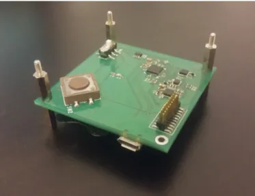
A hardware platform, consisting of all three sensors, has been designed to allow data samples acquisition. The de-vice consists of MAG31103 [2] - a 3D magnetometer and LSM6DS3 [3] - a 3D accelerometer and 3D gyroscope com-bined in one chip. The onboard microcontroller is programmed to obtain the maximum possible sample rate from each sensor and tag each sample with a precise timestamp value. The timestamp is required for each sample, as sensors operate with different frequencies (80Hz and 1666Hz). The timestamp al-lows for precise sample to sample alignment between sensors, which is necessary for the further cross–sensor calibration. The device communicates with a PC using a USB port for data transfer. Using bare hardware for data acquisition allows algorithm generalization, making the developed software im-plementation as universal as possible - it abstracts from the
Author is with the Institute of Computer Science, Warsaw University of Technology, Poland (e-mail: [email protected]).
hardware used and works on raw data, which makes it possible to be used in various applications. Picture of the hardware platform is shown in the Figure 1.
Fig. 1. Hardware platform for data acquisition.
III. CALIBRATION LEVEL
An inertial navigation is a device consisting of a few sensors (three in this case). In such application a two level calibration must be considered. At first, each of the sensors must be calibrated separately. The second step is a calibration which applies to the whole device. This paper focuses on the first stage of this process - a separate calibration for each of the three sensors:
• 3D Magnetometer
• 3D Accelerometer
• 3D Gyroscope
The second calibration step is a sensor–to–sensor orientation calibration. It is a misalignment compensation of the sensors, placed on a surface of printed circuit board. The second stage also includes a gain calibration for the gyroscope device. Its calibration in the first stage would require a usage of some ad-ditional equipment, allowing to apply a rotation of a precisely known angle. The presented algorithms have been prepared, so that they may be used without a need for additional tools. Higher precision algorithms may be developed, but they would require device leveling or a precise rotation, which is not discussed in this article.
IV. DEVICE DISORTION MODEL
At first, a device model must be defined. Separate calibra-tion of each, of the discussed devices, can take an advantage of
using the same model for each sensor, thus allowing to use a similar algorithm in each case. The main diffference between calibration of each sensor is the ammount of data samples collected and thus the number of parameters calculated for the model. In the case of accelerometer sensor, it is more difficult to obtain many samples, so the model must be simplified. Details are discussed further, but a universal model can be described as follows.
A 3D sensor produces a 3D vector at its output. This vector is subjected to two types of disortion. The first one is an independent constant disortion. The second one is a disortion dependent on the current device input value. These disortions combined together are applied by the device and its ambient and influence the produced samples.
Sp= (W ·S) +V0 (1)
Equation 1 shows how each sample is influenced by both disortions. The vector S represents the real value of the measured physical quantity. It is firstly influenced by the matrix W, representing the dependent disortion. This matrix is a symmetric matrix [4] (this implies that no rotation can be introduced to the sample vector, as a rotation matrix would not be symmetric). Its diagonal consists of values close to the value of 1. They represent a gain coefficient within each of the device axes. Rest of the matrix parameters represent non– orthogonalities between the device axes. These valuse are close to 0. The second, constant disortion is represented by vector
V0. It may be interpreted as an offset vector added to each
output sampleSp.
In a perfect situation, when no disortion is introduced, the model parameters would have neutral values as presented in Equation 2. Zero offset vector added to the sample, a matrix representing a unit gain within each axis and no non– orthogonalities between axes. However, a perfect situation will not occur, so these values will be slightly different in a real situation, but still close to the following:
W0= 1 0 0 0 1 0 0 0 1 ,V00= 0 0 0 (2)
A sensor having suchW0andV00values would be an ideal sensor, introducing no disortions (as shown in Equation 3).
Sp= (W0·S) +V00=S (3) Knowing the exact values of the disortion model allows to calculate the inverse of the model presented in Equation 1 and apply it to the samples collected. The inverse model is shown in Equation 4.
S=W−1·(Sp−V0) (4)
At this point it is necessary to obtain the values of W−1
andV0. Having these values allows to calculate the real signal
valueS, for a sampleSp, acquired by the sensor.
V. MODEL PARAMETER ESTIMATION
To estimate the disortion model parameters, an observation may be utilized, that the magnitudes of magnetic field and gravity vectors have fixed values. Regardless of the device orientation, these vectors always lie on a sphere of the radius equal to the vector magnitude and a middle in the point[0,0,0]T. This information is enough to estimate model
parameters. As the model introduces no rotation, there is no need to consider direction of the device. After applying the inverse disortion model (Equation 4) vector S has its origin in the point[0,0,0]T and a constant magnitude ofS. It must be considered that each collected sample was subjected to some noise, thus even after applying the inverse disortion model, it will not be a perfect representation of the physical field vector. This noise is represented as theri part of the Equation 5 and
states for the vector magnitude noise. In fact it is a squared magnitude error, but it is different for each sample i.
ri=STiSi−S2 (5)
Having many data samples collected from the sensor allows the algorithm to estimate the unknown model parameters by minimizing P - a sum of squared noise parts of N samples (Equation 6). P = N X i=1 r2i = = N X i=1 (STiSi−S2)2= = N X i=1 ((W−1·(Spi−V0))T·(W−1·(Spi−V0))−S 2)2= = N X i=1 ((Spi−V0)T ·W−2·(Spi−V0)−S 2)2 (6) W−1= w1 w4 w5 w4 w2 w6 w5 w6 w3 ,V0= x0 y0 z0 (7)
Equation 6 is true, as the matrix W−1 is symmetric (Equation 7). The unknown parameters in this model are [w1, w2, w3, w4, w5, w6, x0, y0, z0, S2]T. The total of 10 un-known parameters require at least 10 samples to be collected to give any results, although the more samples are provided, the more precise the model estimation is expected to be.
If all the unknown parameters are to be estimated, the analytical solution of this problem becomes nonlinear. Two methods have been presented to simplify the calculations. The first one is an analytical method divided into two steps and the second one is numerical solution. The process of collecting the appropriate set of samples, together with results, have been described in further sections.
A. Two–step analytical parameter estimation P = N X i=1 ((Bpi−V0)T ·W−2·(Bpi−V0)−B) 2 (8)
Altough the Equation 8 presents the full analytical definition of the problem, it is nonlinear, and thus not trivial to solve. Thus a different approach has been presented. The process of finding unknown parameters has been divided into two steps. At first theV0 vector and S parameters are estimated, while
temporarily assuming theW−1matrix to be a unit matrix. In the second step, having the first two parameters estimated, the non–linearity matrix is considered unknown, and calculated. These two problems are easier to solve separately. A general method for solving such problems has been described in [2]. Figure 2 presents the algorithm written as a Matlab script.
samples=sample_vector; % step #1
x=[samples,ones(size(samples,1),1)]; y=sum(samples.ˆ2,2);
beta=(x’*x)ˆ(-1)*x’*y;
% vector V0 and magnitude S estimation
V0=beta(1:3,:)./2; S=sqrt(beta(4)+V0’*V0);
% hard-iron calibration application samples=samples-V0’; % step #2 x=[samples.ˆ2, samples(:,1).*samples(:,2), samples(:,1).*samples(:,3), samples(:,2).*samples(:,3)]; y=ones(size(samples,1),1)*(Sˆ2); beta=(x’*x)ˆ(-1)*x’*y;
% matrix W_inv estimation
W_inv=[beta(1), beta(4)/2, beta(5)/2; beta(4)/2, beta(2), beta(6)/2;
beta(5)/2, beta(6)/2, beta(3)]ˆ(0.5);
Fig. 2. Parameters V0 (V0), S (S) and W inv (W−1) analytical estimation.
B. Numerical parameter estimation
The Equation 8 can also be solved numerically. The source code is presented in the Figure 3 and Figure 4. It assumes a fixed magnitude S value, calculated by the analytical method and the starting point for the minimization algorithm is also taken from the previous results.
VI. MAGNETIC FIELD SENSOR
A 3D magnetometer is a device, which measures the mag-netic field vector. The purpose of using a magnetometer in an
samples=sample_vector;
% V0 and S initial values taken
% from 2-step analytical method
beta=fminunc( @(x)performance_function(x, S, samples), [V0;1;1;1;0;0;0], optimoptions(’fminunc’, ’Algorithm’, ’quasi-newton’, ’MaxFunctionEvaluations’, 30000, ’MaxIterations’, 2000)); V0=beta(1:3);
W_inv=[beta(4), beta(7), beta(8); beta(7), beta(5), beta(9); beta(8), beta(9), beta(6)];
Fig. 3. Parameters V0 (V0) and W inv (W−1) numerical estimation. function p=performance_function(x, magnitude, data) v=repmat(x(1:3),1,size(data,1)); W_inv=[x(4),x(7),x(8); x(7),x(5),x(9); x(8),x(9),x(6)]; r=sqrt(sum((W_inv*(data’-v)).ˆ2,1))-magnitude; p=sqrt(r*r’/size(data,1));
Fig. 4. Performance function used in numerical algorithm.
inertial navigation device is to measure the Earths magnetic field. The measured value is altough not only the Earths magnetic field vector. Each sample is a result of superposition of different magnetic fields, caused by various sources. When considering a magnetic field sensor, two types of disortion must be considered [2]:
• The first is hard–iron disortion type. It is a constant
disortion, which is caused by the sensor chip die itsself, by the PCB on which the sensor is mounted and by other objects placed on the PCB. The hard–iron disortion is modelled as a constant offset vector V0, added to each sample produced by the sensor.
• The soft–iron disortion is on the other hand, a non– constant disotrion, dependent on the current orientation of the device. It consists of a gain difference within each of the three axes and a cross–axis non–orthogonality. It is represented by the matrix W in the general model.
A. Sample acquisition
Calibration algorithm requires a set of samples to be col-lected from the sensor. These samples must be colcol-lected in
a specific way, allowing an estimation of all the unknown parameters of the model.
• The first requirement is that each sample must represent a vector of constant magnitude (the magnitude must be constant among all the samples).
• The second requirement is that the collected samples should equally cover all the possible device orientations. This is obviously not a very critical condition, as all the samples are to be collected by rotating the device by hand, but the sample density should be spread among all the possible directions [5].
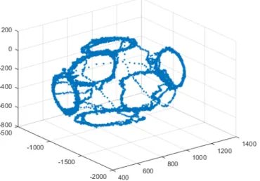
In the case of magnetometer both conditions are met when the samples are to be collected by hand. Regardless of the device orientation or rotation speed, the Earths magnetic field vector has always the same magnitude, so the first requirement is satisfied. To obtain a set of samples covering the whole device sensing range, it is necessary to rotate the device on a flat surface. This provides a sample set forming a circle on some plane within the sensor sensing scope. Repeating this process in each of the following device orientations provides a reasonable set of samples: axis facing the flat surface +X, -X, +Y, -Y, +Z, -Z.
Fig. 5. Magnetometer learning samples set.
Sample acquisition process described, results in the sample set presented in Figure 5.
B. Calibration results
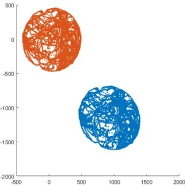
The calibration has been computed using a learning sample set and the algorithm described above. A separate - test sample set has been used for testing purposes. After calculating the magnetometer model parameters, a test has been held, to measure if the computed calibration gives resonable results. The Figure 6 and Figure 7 present the calibration results for both 2–step analytical calibration and numerical calibration.
Magnitude error has been computed for a test sample set (Figure 8), giving a magnitude relative mean squared error of:
• 0.0898 for 2–step analytical calibration
• 0.0929 for numerical calibration
S = 438.1713 V0 = 883.9 −1137.0 −304.9 W−1 = 0.9631 0.0589 −0.0147 0.0589 0.9965 0.0110 −0.0147 0.0110 1.0417
Fig. 6. Magnetometer 2–step analytical calibration results.
S = 438.1713 V0 = 884.7 −1135.1 −303.2 W−1 = 0.9619 0.0568 −0.0142 0.0568 1.0013 0.0113 −0.0142 0.0113 1.0463
Fig. 7. Magnetometer numerical calibration results.
VII. ACCELEROMETER CALIBRATION
Accelerometer is a sensor that measures the accelerations applied to it. Additionaly to the gravity vector it measures all the movement it is subjected to. Because of that, it requires different approach than magnetometer sensor, in terms of sample acquisition.
A. Sample acquisition
Samples for accelerometer calibration can only be collected when the device is in stable position (no movement). Ac-quisition while movement would cause measurement of the gravity vector together with this movement summed together. This would affect magnitude of the measured vector, which is expected to be constant throughout the measurement period. For this research, samples for accelerometer calibration have been collected in a few device orientations, while the device was not moved. The device had been tilted in four ways in a straight position and in an upside down position, giving the total of 8 orientations (Figure 9). In each orientation there have been a few hundreds samples collected. However, because of a little number of orientations covered, the number of unknown parameters had been reduced, to make estimation of the remaining parameters more reliable - the non–orthogonality parameters (w4,w5,w6) have been nulled [6].
B. Calibration and results
The results of both 2–step analytical and numerical calibra-tion are the same (Figure 10 and Figure 11). This is a result of little number of orientations covered. Both algorithms have easily found parameter values for a precise fit, for the given set of learning samples.
Magnitude error has been computed for the test sample set (Figure 12), giving a magnitude relative mean squared error of:
Fig. 8. Magnetometer test samples set (X-Y plane) - raw (blue) and after calibration (orange).
Fig. 9. Accelerometer learn samples set.
• 0.0037 for 2–step analytical calibration
• 0.0037 for numerical calibration
S = 8215.5 V0 = −15.5427 −17.7801 −45.0145 W−1 = 0.9992 0 0 0 1.0070 0 0 0 0.9939
Fig. 10. Accelerometer analytical calibration results.
S = 8215.5 V0 = −15.5427 −17.7801 −45.0145 W−1 = 0.9992 0 0 0 1.0070 0 0 0 0.9939
Fig. 11. Accelerometer numerical calibration results.
Fig. 12. Accelerometer test samples set (X-Z plane) - raw (blue) and after calibration (orange).
C. Comparsion to magnetometer calibration results
The error for accelerometer calibration is significantly lower than the computed error for magnetometer case. This is a result of two facors. At first, the number of orientations at which samples were collected for the accelerometer calibration was lower. Learning set and test set were both collected within the
Fig. 15. Gyroscope test samples set X, Y, Z output at zero rotation -calibration applied.
same orientations - this caused the non–orthogonality error to be excluded in this case. The second factor was that the samples for magnetometer calibration were spread around the coordinate system with different density. As a result, the algorithm fit the calibration model more in the areas containing more samples and less where the sample density was lower.
Both these factors refer to sample acquisition process, which requires some refinig to be done in further research.
VIII. GYROSCOPE CALIBRATION
As the gyroscope shows angular rotation speed, not the angular position, obtaining a constant vector at the output of the sensor would require applying a constant speed rotation to the device. This would require additional equipment, so the process of recognizing matrix W−1 has been ommited for the gyroscope. This parameter can be computed at the next calibration stage - cross sensor calibration - because it is required to know the angle of rotation applied to the device. This angle can be determined by other sensors (magnetometer in particular). Thus the gyroscope calibration at this stage only covers the offset calibration.
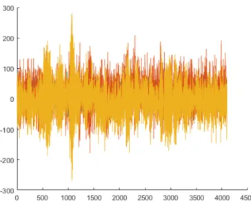
Samples for gyroscope calibration have been collected at a few static positions of the device. Learning sample set is presented in Figure 14. The offset calibrated gyroscope output is shown in the Figure 15 and the results are shown in Figure 13. V0= 883.9 −1137.0 −304.9
Fig. 13. Gyroscope calibration results.
Fig. 14. Gyroscope test samples set - X, Y, Z output at zero rotation - no calibration.
IX. SUMMARY
The presented calibration method is universal and can be applied to any 3D sensor, where a constant magnitude vector samples can be obtained. In the case of an IMU, a calibration of gyroscope gain is necessary to be done separately. This is a part of a second stage calibration - cross sensor calibration. Collecting more samples for the accelerometer calibration can also allow the non–orthogonality parameters to be computed.
REFERENCES
[1] Skog, Isaac, and Peter Hndel. ”Calibration of a MEMS inertial measure-ment unit.” XVII IMEKO World Congress. 2006.
[2] Freescale Semiconductor: Xtrinsic MAG3110 Three-Axis, Digital Mag-netometer
[3] STMicroelectronics: iNEMO inertial module: always-on 3D accelerome-ter and 3D gyroscope
[4] Ozyagcilar, Talat. ”Calibrating an ecompass in the presence of hard and soft-iron interference.” Freescale Semiconductor Ltd (2012).
[5] Pedley, Mark. ”High precision calibration of a three-axis accelerometer.” Freescale Semiconductor Application Note 1 (2013).
[6] Lee, Dongkyu, et al. ”Test and error parameter estimation for MEMS-based low cost IMU calibration.” International Journal of Precision Engi-neering and Manufacturing 12.4 (2011): 597-603.