A deterministic approach to regularized linear discriminant analysis
Alok Sharma
a,b,n, Kuldip K. Paliwal
aa
School of Engineering, Griffith University, Brisbane, QLD, Australia b
School of Engineering and Physics, University of the South Pacific, Suva, Fiji
a r t i c l e i n f o
Article history:Received 19 January 2014 Received in revised form 25 September 2014 Accepted 26 September 2014 Communicated by D. Tao Available online 8 October 2014 Keywords:
Linear discriminant analysis (LDA) Regularized LDA
Deterministic approach Cross-validation Classification
a b s t r a c t
The regularized linear discriminant analysis (RLDA) technique is one of the popular methods for dimensionality reduction used for small sample size problems. In this technique, regularization parameter is conventionally computed using a cross-validation procedure. In this paper, we propose a deterministic way of computing the regularization parameter in RLDA for small sample size problem. The computational cost of the proposed deterministic RLDA is significantly less than the cross-validation based RLDA technique. The deterministic RLDA technique is also compared with other popular techniques on a number of datasets and favorable results are obtained.
&2014 Elsevier B.V. All rights reserved.
1. Introduction
Linear discriminant analysis (LDA) is a popular technique for dimensionality reduction and feature extraction. Dimensionality reduction is a pre-requisite for many statistical pattern recognition techniques. It is primarily applied for improving generalization capability and reducing computational complexity of a classifier. In LDA the dimensionality is reduced fromd-dimensional space to
h-dimensional space (where hod) by using a transformation
WAℝdh. The transformation (or orientation) matrixWis found
by maximizing the Fisher’s criterion:Jð Þ ¼ jW WTS
BWj=jWTSWWj,
where SWAℝdd is within-class scatter matrix and SBAℝdd is
between-class scatter matrix. Under this criterion, the transforma-tion of feature vectors from higher dimensional space to lower dimensional space is done in such a manner that the between-class scatter in the lower dimensional space is maximized and within-class scatter is minimized. The orientation matrix W is computed by the eigenvalue decomposition (EVD) ofSW1SB[1].
In many pattern classification applications, the matrix SW
becomes singular and its inverse computation becomes impossi-ble. This is due to the large dimensionality of feature vectors compared to small number of vectors available for training. This is known as small sample size (SSS) problem [2]. There exist several techniques that can overcome this problem[3–11,19–34]. Among these techniques, regularized LDA (RLDA) technique[3]is
one of the pioneering methods for solving SSS problem. The RLDA technique has been widely studied in the literature[12–14]. It has been applied in areas like face recognition [13,14]and bioinfor-matics[15].
In the RLDA technique, theSW matrix is regularized to
over-come the singularity problem of SW. This regularization can be
done in various ways. For example, Zhao et al.[12,16,17]have done this by adding a small positive constantα(known as regularization parameter) to the diagonal elements of matrixSW; i.e., the matrix
SW is approximated by SWþαI and the orientation matrix is
computed by EVD of ðSWþαIÞ1SB. The performance of RLDA
technique depends on the choice of the regularization parameter
α. In the past studies [18], this parameter is chosen rather heuristically, for example, by applying cross-validation procedure on the training data. In the cross-validation based RLDA technique (denoted here as CV-RLDA), the training data is divided into two subsets: training subset and validation subset. The cross-validation procedure searches over afinite range ofαvalues andfinds anα
value in this range that maximizes the classification accuracy over the validation subset. In the cross-validation procedure, the estimate of α depends on the range over which it is explored. For a given dataset, its classification accuracy can vary depending upon the range ofαbeing explored. Since many values ofαhave to be searched in this range, the computational cost of this procedure is quite high. In addition, the cross-validation procedure used in the CV-RLDA technique is biased towards the classifier used.
In order to address these drawbacks of CV-RLDA technique, we explore a deterministic way for finding the regularization para-meterα. This would provide a unique value of the regularization Contents lists available atScienceDirect
journal homepage:www.elsevier.com/locate/neucom
Neurocomputing
http://dx.doi.org/10.1016/j.neucom.2014.09.051
0925-2312/&2014 Elsevier B.V. All rights reserved.
nCorresponding author.
parameter on a given training data. We call this approach as the deterministic RLDA (DRLDA) technique. This technique avoids the use of the heuristic (cross-validation) procedure for parameter estimation and improves the computational efficiency. We show that this deterministic approach computes the regularization parameter by maximizing the Fisher’s criterion and its classifi ca-tion performance is quite promising compared to other LDA techniques.
2. Related work
In a SSS problem, the within-class scatter matrixSW becomes
singular and its inverse computation becomes impossible. In order to overcome this problem, generally inverse computation ofSWis
avoided or approximated for the computation of orientation matrix W. There are several techniques that can overcome this SSS problem. One way to solve this problem is by estimating the inverse of SW by its pseudoinverse and then the conventional
eigenvalue problem can be solved to compute the orientation matrix W. This was the basis of pseudoinverse LDA (PILDA) technique [20]. Some improvements of PILDA have also been presented in [28,31]. In Fisherface (PCAþLDA) technique,
d-dimensional features arefirstly reduced toh-dimensional fea-ture space by the application of PCA [2,52,53] and then LDA is applied to further reduce features to k dimensions. There are several ways for determining the value ofhin PCAþLDA technique
[4,5]. In the Direct LDA (DLDA) technique[7], the dimensionality is reduced in two stages. In thefirst stage, a transformation matrix is computed to transform the training samples to the range space of
SB, and in the second stage, the dimensionality of this transformed
samples is further transformed by some regulating matrices. The Improved DLDA technique [11], addresses drawbacks of DLDA technique. In the improved DLDA technique, first SW is
decom-posed into its eigenvalues and eigenvectors instead ofSBmatrix as
of DLDA technique. Here, both its null space and range space information are utilized by approximatingSWby a well
determi-nistic substitution. Then SB is diagonalized using regulating
matrices. For the Null LDA (NLDA) technique[6], the orientation
W is computed in two stages. In the first stage, the data is projected on the null space ofSWand in the second stage itfinds
Wthat maximizesjWTSBWj. In orthogonal LDA (OLDA) technique
[8], the orientation matrix W is obtained by simultaneously diagonalizing scatter matrices. It has shown that OLDA is equiva-lent to NLDA under a mild condition [8]. The Uncorrelated LDA (ULDA) technique[21], is a slight variation of OLDA technique. In ULDA, the orientation matrix W is made uncorrelated. The fast NLDA (FNLDA) technique[25], is an alternative method of NLDA. In this technique, the orientation matrix is obtained by using the relationW¼STþSBY, whereYis a random matrix of rankc1, and
c is the number of classes. This technique is so far the fastest technique of performing null LDA operation. In extrapolation LDA (ELDA) technique[32], the null space ofSW matrix is regularized
by extrapolating eigenvalues of SW using exponential fitting
function. This technique utilizes range space information and null space information of SW matrix. The two stage LDA (TSLDA)
technique [34], exploits all four informative spaces of scatter matrices. These spaces are included in two separate discriminant analyses in parallel. In thefirst analysis, null space ofSWand range
space ofSBare retained. In the second analysis, range space ofSW
and null space of SB are retained. In eigenfeature regularization
(EFR) technique [10], SW is regularized by extrapolating its
eigenvalues in its null space. The lagging eigenvalues of SW is
considered as noisy or unreliable which are replaced by an estimation function. The general tensor discriminant analysis (GTDA) technique[48]has been developed for image recognition
problems. This work focuses on the representation and pre-processing of appearance-based models for human gait sequences. Two models were presented: Gabor gait and tensor gait. In[49], authors proposed a constrained empirical risk minimization fra-mework for distance metric learning (DML) to solve SSS problem. In double shrinking sparse dimension reduction technique[50], the SSS problem is solved by penalizing the parameter space. A detailed explanation regarding LDA is given in[51]and an over-view regarding SSS based LDA techniques is given in[47]. There are other techniques which can solve SSS problem and applied in various fields of research [54–62]. In this paper, we focus on regularize LDA (RLDA) technique. This technique overcomes SSS problem by utilizing a small perturbation to theSW matrix. The
details of RLDA have been discussed in the next section.
3. Regularized linear discriminant techniques for SSS problem
In the RLDA technique, the within-class scatter matrix SW is
approximated by adding a regularization parameter to make it a non-singular matrix [3]. There are, however, different ways to perform regularization (see for details,[3,12–14,16,17,30,33]). In this paper we adopted Zhao’s model[12,16,17]to approximateSW
by adding a positive constant in the following wayS^W¼SWþαI.1
This will make within-class scatter matrix a non-singular matrix and then its inverse computation would be possible. The RLDA technique computes the orientation matrixWby EVD of S^W1SB.
Thus, this technique uses null space ofSW, range space ofSWand
range space ofSBin one step (i.e., simultaneously).
In the RLDA technique, a fixed value of regularization para-meter can be used, but it may not give the best classification performance as shown inAppendix B. Therefore, the regulariza-tion parameter α is normally computed by the cross-validation procedure. The cross-validation procedure (e.g. leave-one-out or
k-fold) employs a particular classifier to estimateα and is con-ducted on the training set (which is different from the test set). We briefly describe below the leave-one out cross-validation proce-dure used in the CV-RLDA technique. Let½a;bbe the range ofαto be explored andα0 be any value in this range. Consider a case
when n training samples are available. The training set is first subdivided into training subset (consisting ofn1 samples) and validation subset (consisting of 1 sample). For this particular subdivision of training set, the following operations are required: (1) computation of scatter matricesSB,SW andS^W¼SWþα0Ifor
n1 samples in the training subset; (2) EVD ofS^W1SBto compute
orientation matrixW; and (3) classification of the left out sample (from the validation subset) by the classifier to obtain the classification accuracy. These computational operations are carried out for n1 subdivisions of the training set and the average classification accuracy over the n1 runs is computed. This average classification accuracy is obtained for a particular value ofα (namely α0). All the above operations will be repeated for
other values of α in the range ½a;b to get the highest average classification accuracy. From this description, it is obvious that the cross-validation procedure used in the CV-RLDA technique has the following drawbacks:
Since the cross-validation procedure repeats the above-mentioned computational operations many times for different values ofα, its computation complexity is extremely large.1
In the Friedman’s model[3],SWis estimated asSW^ ¼ð1αÞSWþαI. We have compared Zhao’s model and Friedman’s model of CV-RLDA and found that Zhao’s model exhibits comparatively better generalization capability (seeAppendix Afor details). Furthermore, we have considered Zhao’s model because it is relatively simpler for establishing deterministic approach of computingα(in DRLDA).
In our proposed DRLDA technique, we use a deterministic approach to estimateα parameter by maximizing the modified Fisher’s criterion. The proposed technique is described in the next section.
4. DRLDA technique 4.1. Notations
Let X ¼ fx1;x2;…;xngdenotesntraining samples (or feature
vectors) in ad-dimensional space having class labelsΩ¼ fω1;ω2;
…;ωng, whereωAf1;2;…;cgandcis the number of classes. The set
X can be subdivided intocsubsets X1, X2,…, Xcwhere Xjbelongs to
classjand consists ofnjnumber of samples such that:
n¼ ∑c
j¼1
nj
and XjX and X1[X2[…[Xc¼X.
Ifμjis the centroid of Xjandμis the centroid of X, then the total
scatter matrix ST, within-class scatter matrix SW and
between-class scatter matrixSBare defined as[1,35,36]
ST¼ ∑ xAχðxμÞðxμÞ T ; SW¼ ∑ c j¼1x∑Aχj xμj xμj T ; andSB¼∑cj¼1nj μjμ μjμ T .
Since for SSS problem d4n, the scatter matrices will be singular. It is known that the null space ofST does not contain
any discriminant information[19]. Therefore, the dimensionality can be reduced fromd-dimensional space tort-dimensional space
(wherert is the rank ofST) by applying PCA as a pre-processing
step. The range space ofST matrix,U1Aℝdrt, will be used as a
transformation matrix. In the reduced dimensional space the scatter matrices will be given by:Sw¼UT1SWU1andSb¼UT1SBU1.
After this procedureSwAℝrtrt andSbAℝrtrtare reduced
dimen-sional within-class scatter matrix and reduced dimendimen-sional between-class scatter matrix, respectively.
4.2. Deterministic approach to regularized LDA
In the SSS problem,Swmatrix becomes singular and its inverse
computation becomes impossible. In order to overcome this drawback, the RLDA technique adds a small positive constant α
to all the diagonal elements of matrixSwto make it non-singular;
i.e.,Sw is replaced byS^w¼SwþαI. In this section, we describe a
procedure to compute the regularization parameterα determinis-tically. In RLDA, the modified Fisher’s criterion is given as follows:
^
Jðw;αÞ ¼ wTSbw
wTðS
wþαIÞw ð
1Þ
wherewAℝrt1is the orientation vector. Let us denote a function f¼wTS
bw ð2Þ
and a constraint function
g¼wTðS
wþαIÞwb¼0 ð3Þ
whereb40 is any constant. Tofind the maximum offunder the constraint, let us define a functionF¼fλg, whereλis Lagrange’s multiplier (λa0). By setting its derivative to zero, we get
∂F ∂w¼2Sbwλð2Swwþ2αwÞ ¼0 or 1 λSbSw w¼αw: ð4Þ
Substituting value ofαwfrom Eq.(4)into Eq.(3), we get
g¼wTS
wwþwTð1λSbSwÞwb¼0
or wTS
bw¼λb: ð5Þ
Also from Eq.(3), we get
wTðS
wþαIÞw¼b: ð6Þ
Dividing Eq.(5)by Eq.(6), we get
λ¼ wTSbw
wTðS
wþαIÞw ð
7Þ
The right-hand side of Eq.(7)is same as the criterion^Jðw;αÞ
defined in Eq.(1). The left-hand side of Eq.(7)is the Lagrange’s multiplier (in Eq.(4)). Since our aim is to maximize the modified Fisher’s criterion ^Jðw;αÞ, we must set λ equal to maximum of
^
Jðw;αÞ. However, it is not possible tofind the maximum of^Jðw;αÞ
asαis not known to us. So, as an approximation we setλequal to the maximum of the original Fisher’s criterion (wTS
bw=wTSww). In
order to maximize the original Fisher’s criterion, we must have eigenvectorwto correspond to the maximum eigenvalue ofSw1Sb.
Since in SSS problem Sw is singular and non-invertible, we
approximate the inverse of SW by its pseudoinverse and carry
out the EVD of SwþSbtofind the highest (or leading) eigenvalue,
where Swþ is the pseudoinverse ofSw. Thus, if λmax denotes the
highest eigenvalue of^Jðw;αÞ, then
λmax¼ max w TS bw wTðS wþαIÞw max w TS bw wTS ww largest eigenvalue ofSwþSb ð8Þ
Thereby, the evaluation ofαcan be carried out from Eq.(4)by doing EVD of 1
λSbSw
, whereλ¼λmax. The EVD of 1λSbSw
will give rb¼rankðSbÞ eigenvalues. Since the highest eigenvalue will
correspond to the most discriminant eigenvector,αis the highest eigenvalue. Therefore, if EVD of 1
λSbSw is given by 1 λSbSw ¼EDbwET ð9Þ
where EAℝrtrt is a matrix of eigenvectors andD
bwAℝrtrt is a
diagonal matrix of corresponding eigenvalues. Now the α para-meter can be computed as
α¼maxDbw ð10Þ
After evaluating α, orientation vectorw can be obtained by performing the EVD ofðSwþαIÞ1Sb; i.e., from
ðSwþαIÞ1Sbw¼γw: ð11Þ
From the rb eigenvectors obtained by this EVD, h (rrb)
eigenvectors corresponding tohhighest eigenvalues are used to form the orientation matrixW.
It can be shown fromLemma 1that for DRLDA technique, its maximum eigenvalue is approximately equal to the highest (finite) eigenvalue of Fisher’s criterion.
Lemma 1. The highest eigenvalue of DRLDA is approximately equivalent to the highest (finite) eigenvalue of Fisher’s criterion. Proof 1. From Eq.(11),
Sbwj¼γjðSwþαIÞwj; ð12Þ
where α is the maximum eigenvalue of ð1=λmaxSbSwÞ (from
Eq. (4)); λmaxZ0 is approximately the highest eigenvalue of
Fisher’s criterionwTS
bw=wTSww(sinceλmax is the largest
eigen-value of SwþSb) [46]; j¼1…rb and rb¼rankðSbÞ. Substituting
αw¼ ð1=λmaxSbSwÞw(from Eq.(4), whereλ¼λmax) into Eq.(12),
we get,
Sbwm¼γmSwwmþγmð1=λmaxSbSwÞwm;
or λmaxγm
Sbwm¼0:
where γm¼ maxðγjÞ and wm is the corresponding eigenvector.
SinceSbwma0 (from Eq.(5)),γm¼λmaxandγjoλmax, wherejam.
This concludes the proof.
Corollary 1. The value of regularization parameter is non-nega-tive; i.e.,αZ0 forrwrrt, wherert¼rankðSTÞandrw¼rankðSwÞ.
Proof. Please seeAppendix C.
The summary of the DRLDA technique is given inTable 1,2. The computational requirement for Step 1 of the technique (Table 1) would be Oðdn2Þ; for Step 2 would be Oðn3Þ; for Step
3 would beOðn3Þ; for Step 4 would beOðn3Þ; and, for Step 5 would
beOðdn2Þ. Therefore, the total estimated for SSS case (dcn) would
beOðdn2Þ.
5. Experimental setup and results
Experiments are conducted to illustrate the relative perfor-mance of the DRLDA technique with respect to other techniques for the following two applications: (1) face recognition and (2) cancer classification. For face recognition, two commonly known datasets namely ORL dataset[37]and AR dataset[38]are utilized. The ORL dataset contains 400 images of 40 people having 10 images per person. We use the dimensionality of the original feature space to be 5152. The AR dataset contains 100 classes. We use a subset of AR dataset with 14 face images per class. We use the dimensionality of feature space to be 4980. For cancer
classification, 6 commonly available datasets are used. All the datasets used in the experimentation are described inTable 2. For some datasets, number of training samples and test samples are predefined by their donors (Table 2). For these datasets, we use test samples to evaluate the classification performance. For some datasets, the training and test samples are not predefined. For these datasets we carried outk-fold cross-validation procedure3to
compute the classification performance, wherek¼3.
The DRLDA technique is compared with the following techni-ques: Null LDA (NLDA)[6], cross-validation based RLDA (CV-RLDA), Pseudo-inverse LDA (PILDA)[20], Direct LDA (DLDA)[7], Fisherface or PCAþLDA[4,5], Uncorrelated LDA (ULDA)[21]and eigenfeature regularization (EFR)[10]. All the techniques are used tofind the orientation matrixWAℝdc1, thereby, transforming the original
space toc1 dimensional space, wherecis the number of classes. Then nearest neighbour classifier (NNC) using Euclidean distance measure is used for classifying a test feature vector.
The setting up of CV-RLDA technique in our experiments is described as follows: the regularization parameterαof CV-RLDA is computed by using leave-one-out cross-validation procedure on the training set. This is done in two steps. In thefirst step, we perform a coarse search forαby dividing the pre-selected range
½104;1 λW(whereλWis the maximum eigenvalue ofSW) into
10 equal intervals and finding the interval whose center value
Table 1 DRLDA technique.
Step 1 Pre-processing stage: apply PCA tofind the range spaceU1Aℝdrtof total scatter matrixSTand transform originald-dimensional data space tort-dimensional data space, wherert¼rankðSTÞ. Find reduced-dimensional between-class scatter matrixSb¼UT
1SBU1and reduced-dimensional within-class scatter matrix Sw¼UT
1SWU1, whereSbAℝrtrtandSwAℝrtrt
Step 2 Find the highest eigenvalueλmaxby performing EVD ofSwþSb Step 3 Compute EVD ofð1=λmaxSbSwÞtofind its highest eigenvalueα
Step 4 Compute EVD ofðSwþαIÞ1SbtofindheigenvectorswjAℝrt1corresponding to the leading eigenvalues, where 1rhrrbandrb¼rankðSbÞ. The eigenvectors wjare column vectors of the orientation matrixW0Aℝrth
Step 5 Find orientation matrixWAℝdhin ad-dimensional space; i.e.,W¼U1W'
Table 2
Datasets used in the experimentation.
Datasets Class Dimension Number of available samples Number of training samples Number of test samples Acute Leukemia [40] 2 7,129 72 38 34 ALL subtype[41] 7 12,558 327 215 112 GCM[42] 14 16,063 198 144 54 Lung Adenocarci-noma[43] 3 7,129 96 ([67,19,10])a – – MLL[44] 3 12,582 72 57 15 SRBCT[45] 4 2,308 83 63 20 Face ORL[37] 40 5,152 400 (10/ class) – – Face AR[38] 100 4,980 1400 (14/ class) – – a
The values in the square parenthesis indicate number of samples per class.
2
Matlab code is available fromhttp://www.staff.usp.ac.fj/~sharma_al/index. htm.
3
In the k-fold cross-validation procedure [39], we first partition all the available samples randomly intokroughly equal segments. Then hold out one segment as validation data and the remainingk1 segments as training data. Using the training data, we applied a discriminant technique to obtain orientation matrix and the validation data to compute classification accuracy. This partitioning of samples and computation of classification accuracy is carried outktimes to evaluate average classification accuracy.
gives the best classification performance on the training set. In the second step, this interval is further divided into 10 subintervals for
fine search and the center value of the subinterval that gives the best classification performance is used as thefinal value of the regularization parameter. Thus, in this procedure, a total of 20αvalues are investigated. The regularization parameters com-puted by CV-RLDA technique on various datasets are shown in
Appendix D.
The classification accuracy on all the datasets using the above mentioned techniques are shown inTable 3(the highest classifi ca-tion accuracies obtained are depicted in bold fonts). It can be seen fromTable 3that out of 8 datasets used, the number of times the highest classification accuracy obtained by NLDA is 2, CV-RLDA is 5, PILDA is 1, DLDA is 1, PCAþLDA is 3, ULDA is 2, EFR is 4 and DRLDA is 6. In particular, DRLDA performs better than CV-RLDA for most of the datasets shown inTable 2(it outperforms CV-RLDA for 3 out of 8 datasets, shows equal classification accuracy for 3 datasets and is inferior to CV-RLDA in the remaining 2 datasets). Note that the CV-RLDA technique when implemented in an ideal form (i.e., whenαis searched in the rangeð0;1Þwith infinitely small step size) should give in principle better results than the DRLDA technique. Since it is not possible for practical reasons (i.e., computational cost is infinitely large), afinite range is used in CV-RLDA technique. As a result, DCV-RLDA technique is performing here better in terms of classification accuracy for majority of datasets. In addition, the computational cost of CV-RLDA technique (with α being searched in thefinite range) is considerably higher than the DRLDA technique as shown inTable 4. Here, we measure the CPU time taken by its‘Matlab’program on a Sony computer (core i7 processor at 2.8 GHz).
Furthermore, various techniques using artificial data are experimented. For this, we have created a 2-class problem with initial dimensionsd¼10, 25, 30, 50, and 100. In order to have ill-posed problem, we generated only 3 samples per class. The dimensionality is reduced fromdto 1 for all the techniques and then nearest neighbour classifier is used to evaluate the perfor-mance in terms of classification accuracy. For each dimensiond, the data is created 100 times to compute average classification
accuracy. Table 5depicts the average classification accuracy over 100 runs. It can be observed fromTable 5that EFR technique is not able to perform because of scarce samples. The DRLDA technique and CV-RLDA technique are performing similar. Pseudoinverse technique (PILDA) is performing the lowest as there is not enough information in the range space of scatter matrices.
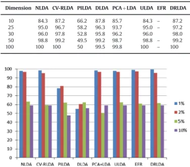
We have also carried out sensitivity analysis with respect to the classification accuracy. For this purpose, we use Acute Leukemia dataset as a prototype and contaminated the dataset by adding Gaussian noise. We then applied techniques again to evaluate classification performance by using nearest neighbor classifier. The generated noise levels are 1%, 2%, 5% and 10% of the standard deviation of the original feature values. The noisy data has been generated 10 times to compute average classification accuracy. The results are shown inFig. 1. It can be observed fromFig. 1that for low level noise the degradation in classification performance is not enough. But when the noise level increases the classification accuracy deteriorates. The performance of PILDA and DLDA tech-niques are lower than other techtech-niques. However, most of the techniques try to maintain the discriminant information in the noisy environment.
6. Discussion
In order to compare the performance in terms of classification accuracy we compared 7 well known techniques with DRLDA. These techniques compute the orientation matrix Wby utilizing different combinations of informative spaces (i.e., null space ofSW,
range space ofSWand range space ofSB). Each informative space
contains a certain level of discriminant information. Theoretically, it is effective to utilize all the informative spaces for the computa-tion of orientacomputa-tion matrix for better generalizacomputa-tion capability. How well a technique is combining these spaces would determine its generalization capability. It has been shown that usually the null space of SW contains more discriminant information than
the range space of SW [6,8,22,34]. Therefore, it is likely that a
technique that utilizes null space ofSW effectively, may perform
Table 3
Classification accuracy (in percentage) on datasets using various techniques. Database NLDA
CV-RLDA
PILDA DLDA PCAþLDA ULDA EFR DRLDA
Acute Leukemia 97.1 97.1 73.5 97.1 100.0 97.1 100.0 100.0 ALL subtype 86.6 95.5 62.5 93.8 80.7 82.1 86.6 93.8 GCM 70.4 74.1 46.3 59.3 59.3 66.7 68.5 70.4 Lung Adeno. 81.7 81.7 74.2 72.0 81.7 80.7 83.9 86.0 MLL 100.0 100.0 80.0 100.0 100.0 100.0 100.0 100.0 SRBCT 100.0 100.0 85.0 80.0 100.0 100.0 100.0 100.0 Face ORL 96.9 97.2 96.4 96.7 92.8 92.5 96.7 97.2 Face AR 95.7 96.3 97.3 96.3 94.9 95.8 97.3 97.3 Table 4
The comparison of cpu time (in seconds) of CV-RLDA and DRLDA techniques. Database CV-RLDA CPU Time DRLDA CPU Time
Acute Leukemia 4.68 0.07 ALL subtype 1021.9 1.90 GCM 265.0 1.26 Lung Adeno. 57.9 0.48 MLL 13.6 0.24 SRBCT 17.0 0.08 Face ORL 7,396.1 7.41 Face AR 739,380 89.9
Fig. 1.Sensitivity analysis of various techniques on Acute Leukemia dataset at different noise levels. They-axis depicts average classification accuracy andx-axis depicts the techniques used. The noise levels are 1%, 2%, 5% and 10%.
Table 5
Classification accuracy (in percentage) on artificial dataset using various techniques.
Dimension NLDA CV-RLDA PILDA DLDA PCAþLDA ULDA EFR DRLDA 10 84.3 87.2 66.2 87.8 85.7 84.3 – 87.2 25 95.0 96.7 58.2 96.3 93.7 95.0 – 97.2
30 96.0 97.8 52.8 95.8 96.2 96.0 98.0
50 98.8 99.2 49.5 99.2 98.7 98.8 – 99.2
better (in generalization capability) than a technique which does not use the null space ofSW.
From the techniques that we have used the NLDA technique employs null space ofSW and range space ofSB. Whereas PILDA,
DLDA and PCAþLDA techniques employ range space ofSW and
range space ofSB. Provided the techniques extract the maximum
possible information from the spaces they employed then NLDA should beat PILDA, DLDA and PCAþLDA techniques. FromTable 3, we can see that NLDA is outperforming PILDA in 7 out of 8 cases. Comparing the classification accuracies of NLDA and DLDA, we can see that NLDA is outperforming DLDA in 4 out of 8 cases and in 2 cases the performance are identical. In a similar way NLDA is surpassing PCAþLDA in 4 out of 8 cases and in 3 cases the performance are identical. On the other hand, the ULDA technique also employs the same spaces as of NLDA technique, however, the classification performance of ULDA is inferior to NLDA (only in 1 out of 8 cases ULDA is beating NLDA). This means that orthogonalWis more effective than uncorrelatedW.
The other three techniques (CV-RLDA, EFR and DRLDA) employ three spaces; namely, null space of SW, range space of SW and
range space ofSB. Intuitively, these three techniques contain more
discriminant information than above mentioned 5 techniques. However, different strategies of using the three spaces would result in different level of generalization capabilities. In CV-RLDA, the estimation of regularization parameter αdepends upon the range ofαvalues being explored (which is restricted due to limited computation time), the cross-validation procedure (e.g. leave-one-out,k-fold) being employed and the classifier used. On the other hand, EFR and DRLDA techniques do not have this problem. The EFR technique utilizes an intuitive model for extrapolating the eigenvalues of range space ofSWto the null space ofSW. This way
it captures all the spaces. However, the model used for extrapola-tion is rather arbitrary and it is not necessary that it is an optimum model. The DRLDA technique captures the information from all the spaces by deterministicallyfinding the optimalαparameter from the training samples. FromTable 3, it can be observed that EFR is surpassing CV-RLDA in 3 out of 8 cases and exhibiting identical classification accuracies in 2 cases. Similarly, DRLDA is outperform-ing CV-RLDA in 3 out of 8 cases and givoutperform-ing equal results in 3 cases. From Tables 3 and 4, we can also observe that though the classification accuracy of CV-RLDA is high (which depends on the search of the regularization parameter), its computational time is extremely large.
Thus we have shown that DRLDA technique is performing better than other LDA techniques for the SSS problem. We can intuitively explain its better performance as follows. In the DRLDA technique, we are maximizing the modified Fisher’s criterion; i.e., the ratio of between-class scatter and within-class scatter (see Eq.
(1)). To get the α parameter, we are maximizing the difference between the between-class scatter and within-class scatter (see Eq.(4)). Thus, we are combining two different philosophies of LDA mechanism in our DRLDA technique and this is helping us in getting better performance.
7. Conclusion
The paper presented a deterministic approach of computing regularized LDA. It avoids the use of the heuristic (cross-validation) procedure for computing the regularization parameter. The techni-que has been experimented on a number of datasets and compared with several popular techniques. The DRLDA technique exhibits highest classification accuracy for 6 out of 8 datasets and its computational cost is significantly less than CV-RLDA technique.
Appendix A
In this appendix, the generalization capabilities of Zhao’s model and Friedman’s model of CV-RLDA are demonstrated on several datasets. In order to do this,first we project the original feature vectors onto the range space of total-scatter matrix as a pre-processing step. Then we employ reduced dimensional within-class scatter matrixS^wfor the two models of CV-RLDA (seeSection
4.1for details about reduced dimensional matrices). In thefirst model of CV-RLDA,Swis approximated asS^w¼SwþαIand in the
second model Sw is approximated as S^w¼ ð1αÞSwþαI. For
brevity, we refer the former model of CV-RLDA as CV-RLDA-1 and the latter model as CV-RLDA-2.Table A1depicts the classifi ca-tion performance of these two models. The details of the datasets and the selection of the regularization parameterαcan be found in
Section 4.
It can be seen fromTable A1that CV-RLDA-1 exhibits relatively better classification performance than CV-RLDA-2.
Appendix B
In this appendix, for RLDA technique we show the sensitivity of classification accuracy when selecting the regularization para-meter, α. For this purpose we use four values of α. These are
δ¼ ½0:001;0:01;0:1;1, whereα¼δλWandλWis the maximum
eigenvalue of within-class scatter matrix. We applied 3-fold cross-validation procedure on a number of datasets and shown the results inTable B1.
It can be observed from the table that the different values of the regularization parameter give different classification accura-cies and therefore, the choice of the regularization parameter affects the classification performance. Thus, it is important to select the regularization parameter correctly to get the good classification performance.
To do this, a cross-validation approach is usually opted. Theα
parameter is searched in the pre-defined range and the value ofα
which gives the best classification performance on the training set is selected. It is assumed that the optimum value ofαwill give the best generalization capability; i.e., the best classification perfor-mance on the test set.
Table A1
Classification accuracy (in percentage) on test set using CV-RLDA-1 and CV-RLDA-2 techniques.
Database CV-RLDA-1 CV-RLDA-2
Acute Leukemia 97.1 97.1 ALL subtype 95.5 86.6 GCM 74.1 70.4 MLL 100.0 100.0 SRBCT 100.0 100.0 Table B1
Classification accuracy (in percentage) using 3-fold cross-validation procedure (the highest classification accuracies obtained are depicted in bold fonts).
Database δ¼0:001 δ¼0:01 δ¼0:1 δ¼1 Acute Leukemia 98.6 98.6 98.6 100 ALL subtype 90.3 90.3 86.0 69.2 GCM 72.7 74.3 76.5 59.0 Lung Adeno. 81.7 80.7 85.0 80.7 MLL 95.7 95.7 95.7 95.7 SRBCT 100.0 100.0 100.0 96.2 Face ORL 96.9 96.9 96.9 96.9 Face AR 95.8 97.9 96.3 81.8
Appendix C
Corollary 1. The value of regularization parameter is non-nega-tive; i.e.,αZ0 forrwrrt, wherert¼rankðSTÞandrw¼rankðSwÞ.
Proof 1. From Eq.(1), we can write
J¼ wTSbw
wTðS
wþαIÞw;
ðA1Þ
where SbAℝrtrt and SwAℝrtrt. We can rearrange the above
expression as
wTS
bw¼JwTðSwþαIÞw ðA2Þ
The eigenvalue decomposition (EVD) ofSW matrix (assuming
rwort) can be given as
Sw¼UΛ2UT, where UAℝrtrt is an orthogonal matrix,
Λ2¼ Λ2w 0 0 0 " # Aℝrtrt and Λ w¼diagðq21;q22;…;q2rwÞAℝ rwrw are
diagonal matrices (asrwort). The eigenvaluesqk240 fork¼1;2;
…;rw. Therefore,
S0w¼ðSwþαIÞ ¼UDUT;whereD¼Λ2þαI
or D1=2UTS0wUD
1=2¼
I ðA3Þ
The between class scatter matrix Sb can be transformed by
multiplyingUD1=2on the right side andD1=2UTon the left side ofSbasD
1=2UTS
bUD
1=2. The EVD of this matrix will give
D1=2UTSbUD1=2¼EDbET; ðA4Þ
where EAℝrtrt is an orthogonal matrix and D
bAℝrtrt is a
diagonal matrix. Eq.(A4)can be rearranged as
ETD1=2UTSbUD1=2E¼Db; ðA5Þ
Let the leading eigenvalue of Db is γ and its corresponding
eigenvector iseAE. Then Eq.(A5)can be rewritten as
eTD1=2
UTSbUD1=2e¼γ; ðA6Þ
The eigenvectorecan be multiplied right side and eT on left
side of Eq.(A3), we get
eTD1=2
UTS0wUD
1=2
e¼1 ðA7Þ
It can be seen from Eqs.(A3) and (A5)that matrixW¼UD1=2E
diagonalizes both Sb and S0w, simultaneously. Also vector
w¼UD1=2e simultaneously gives γ and unity eigenvalues in Eqs. (A6) and (A7). Therefore, w is a solution of Eq. (A2). Substitutingw¼UD1=2ein Eq.(A2), we get
J¼γ; i.e.,wis a solution of Eq.(A2).
From Lemma 1, the maximum eigenvalue of expression
ðSWþαIÞ1Sbw¼γwisγm¼λmax40 (i.e., real, positive andfinite).
Therefore, the eigenvectors corresponding to this positive γm
should also be in real hyperplane (i.e., the components of the vectorwhave to have real values). Sincew¼UD1=2ewithwto
be in real hyperplane, we must haveD1=2to be real. Since D¼Λ2þαI¼diagðq2 1þα;q22þα;…;q2rwþα;α;…;αÞ, we have D1=2¼diagð1= ffiffiffiffiffiffiffiffiffiffiffiffiffiq2 1þα q ;1= ffiffiffiffiffiffiffiffiffiffiffiffiffiq2 2þα q ;…;1= ffiffiffiffiffiffiffiffiffiffiffiffiffiffiq2 rwþα q ;1=pffiffiffiα;…;1=pffiffiffiαÞ:
Therefore, the elements ofD1=2, must satisfy 1= ffiffiffiffiffiffiffiffiffiffiffiffiffiq2
kþα
q
40 and 1=pffiffiffiα40 for k¼1;2;…;rw (note rwort); i.e., α cannot be
negative orα40. Furthermore, ifrw¼rtthen matrixSwwill be a
non-singular matrix and its inverse will exist. In this case, regularization is not required and thereforeα¼0. Thus,αZ0 for
rwrrt. This concludes the proof.
Appendix D
In this appendix, we show computed value of CV-RLDA tech-nique. The value ofαis computed byfirst doing a coarse search on a predefined range tofind a coarse value. After this, afine search is conducted using this coarse value to get the regularization para-meter. In this experiment, we useα¼δλw whereδ¼ ½104;1
andλwis the highest eigenvalue of within-class scatter matrix. The
values are depicted inTable D1. In addition, we have also shown regularization parameters computed by DRLDA technique as a reference.
References
[1]R.O. Duda, P.E. Hart, Pattern Classification and Scene Analysis, Wiley, New
York, 1973.
[2]K. Fukunaga, Introduction to Statistical Pattern Recognition, Academic Press
Inc., Hartcourt Brace Jovanovich, Publishers, 1990.
[3]J.H. Friedman, Regularized discriminant analysis, J. Am. Stat. Assoc. 84 (405) (1989) 165–175.
[4]D.L. Swets, J. Weng, Using discriminative eigenfeatures for image retrieval,
IEEE Trans. Pattern Anal. Mach. Intell. 18 (8) (1996) 831–836.
[5]P.N. Belhumeur, J.P. Hespanha, D.J. Kriegman, Eigenfaces vs. fisherfaces:
recognition using class specific linear projection, IEEE Trans. Pattern Anal. Mach. Intell. 19 (7) (1997) 711–720.
[6]L.-F. Chen, H.-Y.M. Liao, M.-T. Ko, J.-C. Lin, G.-J. Yu, A new LDA-based face recognition system which can solve the small sample size problem, Pattern Recognit. 33 (2000) 1713–1726.
[7]H. Yu, J. Yang, A direct LDA algorithm for high-dimensional data-with
application to face recognition, Pattern Recognit. 34 (2001) 2067–2070. [8]J. Ye, Characterization of a family of algorithms for generalized discriminant
analysis on undersampled problems, J. Mach. Learn. Res. 6 (2005) 483–502.
[9]A. Sharma, K.K. Paliwal, A gradient linear discriminant analysis for small
sample sized problem, Neural Process. Lett. 27 (2008) 17–24.
[10]X. Jiang, B. Mandal, A. Kot, Eigenfeature regularization and extraction in face recognition, IEEE Trans. Pattern Anal. Mach. Intell. 30 (3) (2008) 383–394.
[11] K.K. Paliwal, A. Sharma, Improved direct LDA and its application to DNA gene
microarray data, Pattern Recognit. Lett. 31 (16) (2010) 2489–2492.
[12] W. Zhao, R. Chellappa, P.J. Phillips, Subspace Linear Discriminant Analysis for Face Recognition, Technical Report CAR-TR-914, CS-TR-4009, University of Maryland at College Park, USA, 1999.
[13]D.Q. Dai, P.C. Yuen, Regularized discriminant analysis and its application to face recognition, Pattern Recognit. 36 (3) (2003) 845–847.
[14]D.Q. Dai, P.C. Yuen, Face recognition by regularized discriminant analysis, IEEE Trans. Syst. Man Cybern. Part B Cybern. 37 (4) (2007) 1080–1085.
[15]Y. Guo, T. Hastie, R. Tibshirani, Regularized discriminant analysis and its
application in microarrays, Biostatistics 8 (1) (2007) 86–100.
[16] W. Zhao, R. Chellappa, A. Krishnaswamy, Discriminant analysis of principal components for face recognition, in: Proc. Thir Int. Conf. on Automatic Face and Gesture Recognition, pp. 336–341, Nara, Japan, 1998.
[17] W. Zhao, R. Chellappa, P.J. Phillips, Face recognition: a literature survey, ACM Comput. Surv. 35 (4) (2003) 399–458.
[18]T. Hastie, R. Tibshirani, J. Friedman, The Elements of Statistical Learning,
Springer, NY, USA, 2001.
[19]R. Huang, Q. Liu, H. Lu, S. Ma, Solving the small sample size problem of LDA, Proc. ICPR 3 (2002) 29–32.
[20] Q. Tian, M. Barbero, Z.H. Gu, S.H. Lee, Image classification by the
Foley-Sammon transform, Opt. Eng. 25 (7) (1986) 834–840.
[21] J. Ye, R. Janardan, Q. Li, H. Park, Feature extraction via generalized uncorrelated linear discriminant analysis, in: The Twenty-First International Conference on Machine Learning, pp. 895–902, 2004.
[22] K.K. Paliwal, A. Sharma, Approximate LDA technique for dimensionality
reduction in the small sample size case, J. Pattern Recognit. Res. 6 (2) (2011) 298–306.
Table D1
Computed values of regularization parameter for CV-RLDA and DRLDA on various datasets.
Database CV-RLDA CV-RLDA DRLDA
δ α α Acute Leukemia 0.0057 935.3 6.54109 ALL subtype 0.5056 5.17105 1.111011 GCM 0.0501 2.42104 1.34109 MLL 0.0057 2621.5 2.981010 SRBCT 0.1056 33.01 5715.2
[23]J. Yang, D. Zhang, J.-Y. Yang, A generased K–L expansion method which can deal with small samples size and high-dimensional problems, Pattern Anal. Appl. 6 (2003) 47–54.
[24]D. Chu, G.S. Thye, A new and fast implementation for null space based linear
discriminant analysis, Pattern Recognit. 43 (2010) 1373–1379.
[25]A. Sharma, K.K. Paliwal, A new perspective to null linear discriminant analysis method and its fast implementation using random matrix multiplication with scatter matrices, Pattern Recognit. 45 (6) (2012) 2205–2212.
[26]J. Ye, T. Xiong, Computational and theoretical analysis of null space and
orthogonal linear discriminant analysis, J. Mach. Learn. Res. 7 (2006) 1183–1204.
[27]J. Liu, S.C. Chen, X.Y. Tan, Efficient pseudo-inverse linear discriminant analysis and its nonlinear form for face recognition, Int. J. Pattern Recognit. Artif. Intell. 21 (8) (2007) 1265–1278.
[28] K.K. Paliwal, A. Sharma, Improved pseudoinverse linear discriminant analysis method for dimensionality reduction, Int. J. Pattern Recognit. Artif. Intell. (2011), http://dx.doi.org/10.1142/S0218001412500024.
[29]J. Lu, K. Plataniotis, A. Venetsanopoulos, Face recognition using kernel direct discriminant analysis algorithms, IEEE Trans. Neural Networks 14 (1) (2003) 117–126.
[30]J. Lu, K. Plataniotis, A. Venetsanopoulos, Regularization studies of linear
discriminant analysis in small sample size scenarios with application to face recognition, Pattern Recognit. Lett. 26 (2) (2005) 181–191.
[31]F. Song, D. Zhang, J. Wang, H. Liu, Q. Tao, A parameterized direct LDA and its application to face recognition, Neurocomputing 71 (2007) 191–196. [32]A. Sharma, A., K.K. Paliwal, Regularisation of eigenfeatures by extrapolation of
scatter-matrix in face-recognition problem, IEEE Power Electron. Lett. 46 (10) (2010) 450–475.
[33]J. Lu, K.N. Plataniotis, A.N. Venetsanopoulos, Regularized discriminant analysis for the small sample, Pattern Recognit. Lett. 24 (2003) 3079–3087.
[34]A. Sharma, K.K. Paliwal, A two-stage linear discriminant analysis for
face-recognition, Pattern Recognit. Lett. 33 (9) (2012) 1157–1162.
[35]A. Sharma, K.K. Paliwal, Rotational linear discriminant analysis technique for dimensionality reduction, IEEE Trans. Knowl. Data Eng. 20 (10) (2008) 1336–1347.
[36]A. Sharma, K.K. Paliwal, G.C. Onwubolu, Class-dependent PCA, LDA and MDC: a
combined classifier for pattern classification, Pattern Recognit. 39 (7) (2006) 1215–1229.
[37] F. Samaria, A. Harter, Parameterization of a stochastic model for human face identification, in: Proc. Second IEEE Workshop Applications of Comp. Vision, 138-142, 1994.
[38]A.M. Martinez, Recognizing imprecisely localized, partially occluded, and
expression variant faces from a single sample per class, IEEE Trans. Pattern Anal. Mach. Intell. 24 (6) (2002) 748–763.
[39]E. Alpaydin, Introduction to Machine Learning, MIT Press, 2004.
[40]T.R. Golub, D.K. Slonim, P. Tamayo, C. Huard, M. Gaasenbeek, J.P. Mesirov,
H. Coller, M.L. Loh, J.R. Downing, M.A. Caligiuri, C.D. Bloomfield, E.S. Lander, Molecular classification of cancer: class discovery and class prediction by gene expression monitoring, Science 286 (1999) 531–537.
[41]E.J. Yeoh, M.E. Ross, S.A. Shurtleff, W.K. Williams, D. Patel, R. Mahfouz, F. G. Behm, S.C. Raimondi, M.V. Relling, A. Patel, C. Cheng, D. Campana, D. Wilkins, X. Zhou, J. Li, H. Liu, C.H. Pui, W.E. Evans, C. Naeve, L. Wong, J. R. Downing, Classification, subtype discovery, and prediction of outcome in pediatric acute lymphoblastic leukemia by gene expression profiling, Cancer 1 (2) (2002) 133–143.
[42]S. Ramaswamy, P. Tamayo, R. Rifkin, S. Mukherjee, C.-H. Yeang, M. Angelo,
C. Ladd, M. Reich, E. Latulippe, J.P. Mesirov, T. Poggio, W. Gerald, M.. Loda, E. S. Lander, T.R. Golub, Multiclass cancer diagnosis using tumor gene expression signatures, Proc. Natl. Acad. Sci. U.S.A. 98 (26) (2001) 15149–15154. [43]D.G. Beer, S.L.R. Kardia, C.-C. Huang, T.J. Giordano, A.M. Levin, D.E. Misek, L. Lin,
G. Chen, T.G. Gharib, D.G. Thomas, M.L. Lizyness, R. Kuick, S. Hayasaka, J.M. G. Taylor, M.D. Iannettoni, M.B. Orringer, S. Hanash, Gene-expression profiles predict survival of patients with lung adenocarcinoma, Nat. Med. 8 (2002) 816–824.
[44]S.A. Armstrong, J.E. Staunton, L.B. Silverman, R. Pieters, M.L. den Boer, M.
D. Minden, S.E. Sallan, E.S. Lander, T.R. Golub, S.J. Korsemeyer, MLL transloca-tions specify a distinct gene expression profile that distinguishes a unique leukemia, Nat. Genet. 30 (2002) 41–47.
[45]J. Khan, J.S. Wei, M. Ringner, L.H. Saal, M. Ladanyi, F. Westermann, F. Berthold, M. Schwab, C.R. Antonescu, C. Peterson, P.S. Meltzer, Classification and diagnostic prediction of cancers using gene expression profiling and artificial neural network, Nat. Med. 7 (2001) 673–679.
[46]J. Liu, S.C. Chen, X.Y. Tan, Efficient pseudo-inverse linear discriminant analysis and its nonlinear form for face recognition, Int. J. Pattern Recognit. Artif. Intell. 21 (8) (2007) 1265–1278.
[47] A. Sharma, K.K. Paliwal, Linear discriminant analysis for small sample size problem: an overview, Int. J. Mach. Learn. Cybern (2014), http://dx.doi.org/
10.1007/s13042-013-0226-9.
[48]D. Tao, X. Li, X. Wu, S. Maybank, General tensor discriminant analysis and
Gabor features for gait recognition, IEEE Trans. Pattern Anal. Mach. Intell. 29 (10) (2007) 1700–1715.
[49]W. Bian, D. Tao, Constrained empirical risk minimization framework for
distance metric learning, IEEE Trans. Neural Networks Learn. Syst. 23 (8) (2012) 1194–1205.
[50]T. Zhou, D. Tao, Double shrinking sparse dimension reduction, IEEE Trans.
Image Proc 22 (1) (2013) 244–257.
[51]D. Tao, X. Li, X. Wu, S.J. Maybank, Geometric mean for subspace selection, IEEE Trans. Pattern Anal. Mach. Learn. 31 (2) (2009) 260–274.
[52]A. Sharma, K.K. Paliwal, S. Imoto, S. Miyano, Principal component analysis
using QR decomposition, Int. J. Mach. Learn. Cybern. 4 (6) (2013) 679–683.
[53]A. Sharma, K.K. Paliwal, Fast principal component analysis usingfixed-point
algorithm, Pattern Recognit. Lett. 28 (10) (2007) 1151–1155.
[54]S.-J. Wang, H.-L. Chen, X.-J. Peng, C.-G. Zhou, Exponential locality preserving projections for small sample size problem, Neurocomputing 74 (17) (2011) 3654–3662.
[55]L. Zhang, W. Zhou, P.-C. Chang, Generalized nonlinear discriminant analysis
and its small sample size problems, Neurocomputing 74 (4) (2011) 568–574.
[56]H. Huang, J. Liu, H. Feng, T. He, Ear recognition based on uncorrelated local Fisher discriminant analysis, Neurocomputing 74 (17) (2011) 3103–3113. [57]E.B. Huerta, B. Duval, J.-K. Hao, A hybrid LDA and genetic algorithm for gene
selection and classification of microarray data, Neurocomputing 73 (13-15) (2010) 2375–2383.
[58]A. Sharma, S. Imoto, S. Miyano, A top-r feature selection algorithm for
microarray gene expression data, IEEE/ACM Trans. Comput. Biol. Bioinf. 9 (3) (2012) 754–764.
[59]A. Sharma, S. Imoto, S. Miyano, A between-class overlapping filter-based
method for transcriptome data analysis, J. Bioinf. Comput. Biol. 10 (5) (2012)
1250010–1250011 (1250010-20).
[60]A. Sharma, S. Imoto, S. Miyano, V. Sharma, Null space based feature selection method for gene expression data, Int. J. Mach. Learn. Cybern. 3 (4) (2012) 269–276.
[61]A. Sharma, K.K. Paliwal, Cancer classification by gradient LDA technique using microarray gene expression data, Data Knowledge Eng. 66 (2) (2008) 338–347.
[62]W Yang, H. Wu, Regularized complete linear discriminant analysis,
Neuro-computing 137 (2014) 185–191.
Alok Sharma received the BTech degree from the University of the South Pacific (USP), Suva, Fiji, in 2000 and the MEng degree, with an academic excel-lence award, and the PhD degree in the area of pattern recognition from Griffith University, Brisbane, Australia, in 2001 and 2006, respectively. He is currently a research fellow at the University of Tokyo, Japan. He is also with the Signal Processing Laboratory, Griffith University and the University of the South Pacific. He participated in various projects carried out in conjunc-tion with Motorola (Sydney), Auslog Pty. Ltd. (Bris-bane), CRC Micro Technology (Bris(Bris-bane), and the French Embassy (Suva). He is nominated by NSERC, Canada in Visiting Fellowship program, 2009. His research interests include pattern recogni-tion, computer security, and human cancer classification. He reviewed several articles from journals and is in the Editorial board of several journals.
Kuldip K. Paliwalreceived the B.S. degree from Agra University, Agra, India, in 1969, the M.S. degree from Aligarh Muslim University, Aligarh, India, in 1971 and the Ph.D. degree from Bombay University, Bombay, India, in 1978.
He has been carrying out research in the area of speech processing since 1972. He has worked at a number of organizations including Tata Institute of Fundamental Research, Bombay, India, Norwegian Institute of Technology, Trondheim, Norway, University of Keele, U.K., AT&T Bell Laboratories, Murray Hill, New Jersey, U.S.A., AT&T Shannon Laboratories, Florham Park, New Jersey, U.S.A., and Advanced Telecommuni-cation Research Laboratories, Kyoto, Japan. Since July 1993, he has been a professor at Griffith University, Brisbane, Australia, in the School of Microelectronic Engineer-ing. His current research interests include speech recognition, speech coding, speaker recognition, speech enhancement, face recognition, image coding, pattern recognition and artificial neural networks. He has published more than 300 papers in these research areas.
Prof. Paliwal is a Fellow of Acoustical Society of India. He has served the IEEE Signal Processing Society’s Neural Networks Technical Committee as a founding member from 1991 to 1995 and the Speech Processing Technical Committee from 1999 to 2003. He was an Associate Editor of the IEEE Transactions on Speech and Audio Processing during the periods 1994–1997 and 2003–2004. He is in the Editorial Board of the IEEE Signal Processing Magazine. He also served as an Associate Editor of the IEEE Signal Processing Letters from 1997 to 2000. He was the General Co-Chair of the Tenth IEEE Workshop on Neural Networks for Signal Processing (NNSP2000). He has co-edited two books:“Speech Coding and Synth-esis” (published by Elsevier), and“Speech and Speaker Recognition: Advanced Topics”(published by Kluwer). He has received IEEE Signal Processing Society’s best (senior) paper award in 1995 for his paper on LPC quantization. He served as the Editor-in-Chief of the Speech Communication journal (published by Elsevier) during 2005–2011.