No. 6/2006
Structural change and regional
employment dynamics
Uwe Blien, Helge Sanner
IABDiscussionPaperNo. 6/2006 2
Structural change and regional
Employment dynamics
Uwe Blien (IAB), Helge Sanner (Universität Potsdam)
Auch mit seiner neuen Reihe „IAB-Discussion Paper“ will das Forschungsinstitut der Bundesagentur für Arbeit den Dialog mit der externen Wissenschaft intensivieren. Durch die rasche Verbreitung von Forschungsergebnissen über das Internet soll noch vor Drucklegung Kritik angeregt und Qualität
gesichert werden.
Also with its new series "IAB Discussion Paper" the research institute of the German Federal Employment Agency wants to intensify dialogue with external science. By the rapid spreading of research results via Internet still before printing criticism shall be stimulated and quality shall
Structural change and regional employment
dynamics
Uwe Blien and Helge Sanner
April 7, 2006
Abstract
A casual look at regional unemployment rates reveals that there are vast differences which cannot be explained by different institutional settings. Our paper attempts to trace these differences in the regions’ labour market per-formance back to the regions’ specialisation in products that are more or less advanced in their product cycle. The model we develop shows how individual profit and utility maximisation endogenously leads to decreasing employment in the presence of process innovation. Things deteriorate even further if the region under observation is less innovative than others. Our model suggests that the only way to escape from this vicious circle is to specialize in products that are at the beginning of their economic life.
Keywords: Structural change; Productivity growth; Labour market dynamics; Specialisation of Regions
JEL-codes: O41; D91; J23; R23
1
Introduction
The standard explanation of unemployment is related to the institutional structure behind the labour market. The more flexible the institutional setting is the lower is the unemployment rate. This is the main conclusion drawn from the work of Layard, Nickell and Jackman (1991) and of many followers. However, there is a striking discrepancy between this proposition and (at least) one empirical fact. At regional level, within one country, there are vast disparities between unemployment rates. They are of about the same size as they are between independent countries (Südekum, 2005). The differences in regional unemployment cannot be explained by
different institutional settings, which do not vary much within one country. Therefore, other explanations are required.
In this paper a theoretical model is developed which explains differing employ-ment and then differing unemployemploy-ment paths by structural change. To some extent regions (or nations) are specialized to different products. These products are sub-ject to different demand conditions on their markets and there are specific paths of progress in the production technology. These conditions can be used to explain labour market disparities.
To begin with a rough outline of the argument, two effects of technological progress have to be taken into account. The first is a labour-saving one. Due to productivity gains less labour is required to produce the same amount of products. But then there is a secondary effect working in the opposite direction, because prices decrease as a consequence of technological progress. Lower prices boost product demand, so more labour is needed to produce a larger output. Whether this compen-sating effect outweighs the first labour-saving one is an empirical question. In fact three cases are possible. In the first case the labour-saving effect dominates. In the second case, labour demand remains constant and in the third case labour demand even increases. It is obvious that the elasticity of aggregate demand is decisive for the outcome. As will be shown in this paper, the limiting value — for the case of a one-good economy —is an elasticity level of minus one, under quite general conditions: labour demand increases if product demand is elastic.
Our results regarding the effects of productivity gains on employment are related to structural change, since our framework decidedly points at the dynamic conse-quences of a substitution of one product by another. These conseconse-quences could be quite diverse for the industries, regions, cities and nations that are affected. It is easy to see that productivity increases in a nation’s leading industry can have a pos-itive impact on employment and other important economic variables, whereas in a completely symmetric case detrimental consequences are to be expected if the crucial condition is not met.
In the literature the term structural change is used in a narrow and in a broad sense. Although we usually employ the former interpretation, both of them are com-patible with our analytical framework. In the narrow sense structural change refers to the substitution of one industry by another in a country’s productive capacities. The properties of product cycles may be analysed within the framework presented here. In the broad sense the term structural change is related to the change of proportions between the large sectors of the economy and to the secular expansion of the service sector at the expense of the industrial and agrarian sectors. Again it is possible to
analyse this process from the viewpoint of the employment theorem on structural change.
Standard analyses of economic growth are mainly concerned with productivity developments. The effects on employment are usually ignored and market clearing is assumed. Here, it can be seen that the relationship between technological progress and employment is not a trivial one. A framework is provided which permits a detailed analysis.
We do not claim that the theorem about the effects of productivity increases on employment is completely new. As far as we know a basic version of it was first prop-erly stated in a simple macroeconomic model published in a relatively hidden place (Appelbaum and Schettkat, 1993). Möller (2001) supports its empirical relevance. Recently, versions of the theorem has appeared in prominently placed papers on ag-glomeration effects (see e.g. Cingano and Schivardi (2004) and Combes, Magnac and Robin (2004)). We will show the precise content of the basic Appelbaum/Schettkat theorem in the following section of this paper.
Our main contribution is the development of a still simple, but fully-fledged model which includes a proper micro-foundation of the theorem. This is done in two steps: in the first step, the theorem is derived and generalized to the case of n industries producing goods that may exhibit any sorts of substitutability. In the second step the micro-model is developed, which shows the full dynamics of one good being replaced by another one. Both steps give insights into the conditions that have to be met for the stated consequences of productivity increases on (un-)employment. We will see later, that it is even possible to reconcile the model presented here with the standard macroeconomic approach of Layard et al. and their followers.
The explanation of unemployment from the interaction of product demand, tech-nological progress and structural change would be consistent with many stylized facts about modern economies:
• As stated above, employment in specialized regions could develop very differ-ently – although the regions are comparable with respect to institutions and resources.
• New literature shows that agglomeration effects are empirically important with respect to productivity, but not with respect to employment. The labour market performance of regions with more concentrated industries might even be worse than that of a rural country Combes et al. (2004).
world market, although the average wages paid are about five times higher than those of some main Eastern European competitors. This would indicate that the German economy is specialized on markets with an inelastic demand – at any rate the economy is affected by a severe unemployment problem.
• It is often difficult to derive differences in the unemployment rates of nations from their labour market institutions (cf. the review by Freeman, 2001).
• The relationship between productivity gains and the development of employ-ment changes over time (Cavelaars, 2005). This could be due to shifts on the product market related to the product cycle of some leading industries.
In section 2 the employment effects of productivity gains are traced back to the elasticity of aggregate demand. Our findings are summarized in a basic theorem, as well as a couple of corollaries. In section 3 a microeconomic model is presented that suggests that decreasing price elasticities and thus a decline of employment is an inherent feature of every product cycle. Section 4 discusses the results obtained, and section 5 concludes.
2
Structural change, demand, and employment
Assume an economy whose product market consists of n perfectly competitive in-dustries. Each firm within the same industry exhibits the same linear-homogenous production function.1 Aggregation at the industry level yields the industry-wide pro-duction functions Qj(t) = Aj(t)·f(Kj, Lj), where K and L denote the amount of
capital and labour employed, respectively. The prices of these factors, denotedr and w, are assumed to be constant. Aj(t) =Ajeγjt is an industry-specific scaling factor,
which increases over time twith the exogenous industry-specific rate of technological progress, γj. Labour productivity in industry j isπj(t) =Qj(t)/Lj(t) = Aj(t)·f(kj),
where kj denotes capital intensity, k≡K/L.2
Demand at the industry level κ isQκ(p1, . . . , pκ, . . . , pn), wherepj denote prices
that must be equal for all firms within the same industry j. More specifically, these prices coincide with the marginal costs of production, of which labour costs make up 1This assumption is more than necessarily restrictive, and has primarily been made to ease the presentation. For our results to become effective without qualification, any production function that leads to a constant capital intensity would suffice, e.g. the Leontieff and every homothetic production function.
2Note that k is time-invariant, since we assume homothetic production functions, and factor prices are held constant.
a constant share. Put differently, prices contain a constant mark-up on labour input per unit produced, Lj/Qj = 1/πj, i.e. pj(t) = θj/πj(t), where θj is an
industry-specific parameter which depends on factor prices and the technology employed, but not on time.3 This is to say that prices only change over time in this model because they depend on productivity, ceteris paribus.
Now we are in the position to analyse the development of employment over time. It is appropriate to summarize the functional relationships needed for this exercise:
πj(t) = Qj(t) Lj(t) =Aj(t)·f(kj) (A) Aj(t) =Ajeγjt (B) pj(t) = θj πj(t) (C) Qj(t) = Qj(p1(t), . . . , pj(t), . . . , pn(t)) (D)
Note that equations (A)–(D) are either based on fairly weak and standard precondi-tions, or even definitory.
Building the derivative of the price-setting equation (C) with respect toπj yields
∂pj ∂πj = −θj πj(t)2 = −pj πj(t) (1)
The evolution of employment over time can be inferred by building the total derivative ofLκ =Qκ(p1, . . . , pκ, . . . , pn)/πκ with respect to t:
dLκ dt = 1 πκ2 · " n X j=1 ∂Qκ(·) ∂pj ∂pj ∂πj ∂πj ∂t πκ−Qκ(·) ∂πκ ∂t # (2)
Making use of eq. (1) and ∂πj/∂t=γjπj, the derivative becomes
dLκ dt = −1 πκ2 · " n X j=1 ∂Qκ(·) ∂pj pj πj γjπj πκ+Qκ(·)γκπκ # = −1 πκ · " n X j=1 ∂Qκ(·) ∂pj pj Qκ(·) γjQκ(·) +Qκ(·)γκ # = −γκLκ· " n X j6=κ ηQκ,pj γj γκ +ηQκ,pκ+ 1 # (3)
whereηQκ,pj denotes the elasticity of aggregate demand for commodityκwith respect
to the price of commodity j. While we can safely assume that the direct price 3In the case of a Cobb-Douglas production function,Q
j(t) =Aj(t)Kjβ1Ljβ2, withβ1+β2 R1,
it is straightforward to show that θj =w/β2. Note that only in the casesβ1+β2 ≤ 1 are firms’
elasticity is negative, the sign of the cross-price elasticities depends on whether the goods are substitutesηQκ,pj >0or complementsηQκ,pj <0. If the rate of technological
progress is zero in one specific industry l6=κ, the degree of substitutability between goods l and κ has no effect on the evolution of employment in industry κ. If γκ = 0,
the development of employment in the κ-industry hinges solely on the technological progress in other industries and the corresponding cross-price elasticities:
dLκ dt γκ=0 =−Lκ· n X j6=κ ηQκ,pjγj
The result expressed in eq. (3) is summarized in the following theorem, which thus holds under relatively weak and largely standard restrictions:
Theorem 1 Employment in one specific industry κ rises if, and only if, the sum of all cross-price elasticities of the commodity produced by this industry, weighted by the relative rates of technological progress, plus the direct price elasticity are below minus one.
Two quite interesting corollaries can be deduced from theorem 1.
Corollary 1 (Appelbaum and Schettkat, 1993) For a given technology of all other industries (γj = 0, ∀j 6= κ), technological progress in industry κ leads to an
increase in employment if the price elasticity of demand of the corresponding good is below minus one (see Appelbaum and Schettkat, 1993). If, however, the direct price elasticity is greater than minus one, a higher rate of technological progress in
this industry actually accelerates the decrease in employment due to its labour-saving
effect.
Corollary 2 The more industries produce close substitutes with a high rate of technological progress, the more likely it is that employment in industry κ decreases due to technological progresseven if the demand elasticity for the corresponding good
is well below minus one.
Dividing eq. (3) by Lκ we obtain the growth rate of employment in industry κ:
ˆ Lκ = dLκ/dt Lκ =−γκ· " n X j6=κ ηQκ,pj γj γκ +ηQκ,pκ+ 1 # (4) If the technological growth rates of all industries are equal,γj =γκ, ∀j ∈ {1,· · ·, n},
and the budget constraint yi = Pnj=1pjqj is binding for all consumers i, eq. (4)
reduces to ˆ Lκ = γκ· " n X j=1 ηQκ,pj + 1 # = γκ·(1−Qκ,y) (5)
where Qκ,y denotes the income elasticity of good κ. Eq. (5) suggests that global
technological progress boosts employment in a specific industry if the good produced by this industry is superior, i.e. characterized by a larger proportion of consumption as income rises. Since the income elasticity is one on average, the weighted average growth rate of employment in all industries is zero. In other words, in this fairly stan-dard model framework, global technological progress can only have a positive effect on employment in one region or country if its economy possesses a disproportionately large share of industries with superior goods. Employment gains in this region are accompanied by employment losses in other regions, however.4
The next section depicts the arguments developed in this section by means of a two-industry microeconomic model. We put the changes of the price elasticity in the context of the product cycle. Moreover, by assuming that wages do not fully adjust to changes in the scarcity of labour for whatever reason, we link technological progress and the development of unemployment. Cross-country differences in unemployment are hence explained by technological change, in addition to (partial) stickiness of wages.
3
Structural change, and the dynamics of demand
and unemployment
The model introduced in this section provides a fully-fledged microeconomic basis for the relationships described in the preceding analysis. In particular, we derive that endogenous forces decrease the elasticity of demand over time, so that eventually productivity gains start to have a detrimental effect on employment.
3.1
Setting
Our economy consists of three industries. One perfectly competitive industry pro-duces the homogenous consumption bundle (’the rest of the world’) that serves as a reference throughout the analysis. The two other industries, denoted by the index j ∈ {a, b}, respectively produce an indivisible good (e.g. automobiles) under likewise perfect competition. Consumers either buy one of the indivisible goods produced by 4Of course, this result is sensitive to our assumption that factor prices are constant. Below we will argue that the results are qualitatively the same as long as some sort of stickiness of factor prices can be assumed, e.g. for the more than 40 nations for which researchers have found evidence of a wage curve (see Blanchflower and Oswald, 2005, p. 1).
one of the two industries, or none. The intertemporal utility function to be maximized by each infinitely living and myopic consumer i is
maxvi =
Z ∞
0
ui(t)e−rtdt (6)
wherer denotes the uniform subjective rate of time preference, which is equal to the interest rate, and ui(t)denotes the utility of one consumer in periodt. Period utility
depends in the following way on the amounts consumed:
ui(t) = lnci(t) +qa,i(t) +δqb,i(t); qj,i ∈ {0,1}; ∀i (7)
(qa,i+qb,i)∈ {0,1}; ∀i
δ >0
c denotes consumption of the homogenous consumption bundle. For our results to become effective, it is merely necessary that this part of the additive utility function exhibits decreasing marginal utility. Each consumer may or may not consume one unit of one q-good. The utility contribution of these goods is 1 and δ, respectively. Without loss of generality we assume δ < 1, i.e. consumers prefer the a-good. This implies that the price of the latter must be lower in order to be competitive. Unlike the homogenous consumption bundle, which must be used up immediately, both q -goods yield a utility flow within an interval of length T.
Consumers face the budget constraint
yi =ci(t) +sa(τ)qa(τ) +sb(τ)qb(τ); τ ∈[t, t+T] (8)
where the price of the homogenous consumption bundle is standardized to unity, i.e. this good is taken as the numeraire. An individual’s period income, yi, is assumed to
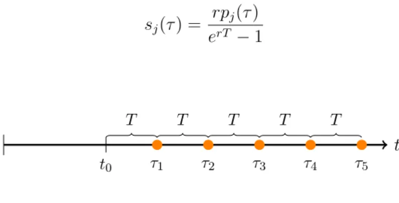
be constant in time. sj are annuities, and stand for the amount that must be saved
each period so that theq-good can be bought in periodτ(either for the first time, or as a replacement, see fig. 1). This amount remains constant within the interval because of the diminishing marginal utility of the composite good and because the individual rate of time preference equals the interest rate. Att0 the considered household starts
to save in order to buy the q-good in τ1 for the first time. Since we will assume a
continuum of different incomes below, the number of consumers who start consuming a q-good at a specific point in time is negligible in relation to the total number of consumers. Notice that consumers must be able to anticipate future prices for our diagram to be exact. From pj(τ) = Z T 0 sj(τ)ertdt
where pj(τ)denotes the price of industry j’s q-good at the moment of the purchase, τ, we obtain sj(τ) = rpj(τ) erT −1 (9) t T T T T T t0 τ1 τ2 τ3 τ4 τ5
Fig. 1: Timeline and moments of replacement
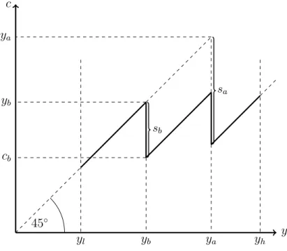
Due to the decreasing marginal utility of the homogenous consumption good, a critical period income exists at which consumers are indifferent between consuming or not consuming one of the q-goods with constant utility. The higher price and utility contribution of thea-good effectuates that this good is purchased by richer households than industry b’s good. Next, we derive the critical incomes ya and yb above which
a consumer respectively purchases industry a’s and industry b’s goods. ca and cb
denote the homogenous good consumption of the marginal consumers, respectively. The marginal consumers of theb-good are indifferent to whether they consume more of the homogenous consumption bundle or whether they buy one unit of good b:
Z T 0 {ln[cb(t)] +δ}e−rtdt= Z T 0 ln[cb(t) +sb(T)]e−rtdt (10)
Due to the decreasing utility of the homogenous consumption bundle, the amount saved in each period must be constant, so the equality between the flows of utility must hold in every period, i.e.
ln[cb(T)] +δ= ln[cb(T) +sb(T)]
cb(T) =
sb(T)
eδ−1
This relationship must hold for each period’s marginal consumer: cb(t) =
sb(t)
eδ−1
The critical income is defined the income of the marginal buyer yb(t) = cb(t) +sb(t) = eδs b(t) eδ−1 (11) = e δ eδ−1 rpb(t) erT −1
The critical incomeyaat which a consumer is indifferent to whether they consume
the a-good and less of the composite good, or the less appreciated b-good and more of the composite good can be derived from the following condition:
Z T 0 {ln[ca(t)] + 1}e−rtdt= Z T 0 {ln[ca(t) +sa(T)−sb(T)] +δ}e−rtdt (12)
Optimality requires that the consumers split the costs of the q-good evenly:
ln[ca(T)] + 1 = ln[ca(T) + (sa(T)−sb(T))] +δ
ca(T) =
sa(T)−sb(T)
e1−δ−1
The critical consumption level ca in period t is
ca(t) =
sa(t)−sb(t)
e1−δ−1
Finally, we can derive the income of the marginal a-consumer as ya(t) = ca(t) +sa(t) = sa(t)e1−δ−sb(t) e1−δ−1 (13) = e1−δp a(t)−pb(t) r (e1−δ−1)·(erT −1)
By means of eq. (11) and (13) we can infer which consumer buys one unit of gooda, one unit of good b, or no q-good at all. As expected, both critical incomes depend negatively on the price of the corresponding good.
Figure 2illustrates the amounts that consumers spend on the consumption bun-dle, or save each period to finance the acquisition of a q-good. Households endowed with an income between yl and yb only buy the consumption bundle (recall that the
price of the consumption bundle is one). Households with an income in the interval
[yb, ya)buy one unit of theb-good and spend the remaining income on the composite
consumption good. All households with an income above ya buy the more expensive
a-good, and y−sa units of the composite good.
3.2
Individual and aggregate production
Assume perfect competition on the market for the homogenous good, as well as on both of the markets for the q-goods. All firms regard input prices and output prices as being given to them exogenously. The production functions for both q-goods is of the Cobb-Douglas type. Since it is linearly homogenous, production functions at the industry level have the same structure:
Qj(t) = Aj(t)Kj(t) β
Lj(t)
1−β
y c yl yb ya cb sb yb sa ya yh 45◦
Fig. 2: Individual income and consumption
whereQ, A, K, L, βand1−βdenote the amount produced, a scale factor, capital em-ployed, labour employed and the partial production elasticities of capital and labour, respectively. The scale factors increase over time due to exogenous technological progress (process innovations) in the following way:
Aj(t) =Ajeγjt
where γj are the industry-specific rates of technological progress. The costs of one
firm ` in the j-industry are
Cj`(t) =rβw1−ββ−β(1−β)−(1−β)Q
` j(t)
Aj(t)
where r and w denote the exogenously determined prices of capital and labour, i.e. capital input is standardized such that its price coincides with the rate of time prefer-ence. Profit maximisation for all identical firms yields that the price equals marginal costs: pj(t) =rβw1−βµ 1 Aj(t) (15) where µ≡β−β(1−β)−(1−β).
Since the scale factors Aj(t) increase over time due to technological progress,
marginal costs and prices are monotonically decreasing functions of time. This implies that the critical incomes,yb(t)andya(t), at which a consumer is indifferent to whether
he buys one specific good or not, decrease over time as well. Since the income differs across consumers but is constant over time, the number of consumers of the two q-goods and aggregate demand increase within a certain range of parameters.
3.3
Aggregate demand and equilibrium
In order to calculate aggregate demand, we need to make an assumption about the distribution of income within the economy. For ease of calculation, we adopt a rect-angular distribution.
g(y) =
(
α ∀y:y∈[yl, yh]
0 else
yl and yh denote minimum and maximum income, respectively. The density of
con-sumers with an income betweenyl and yh is α.
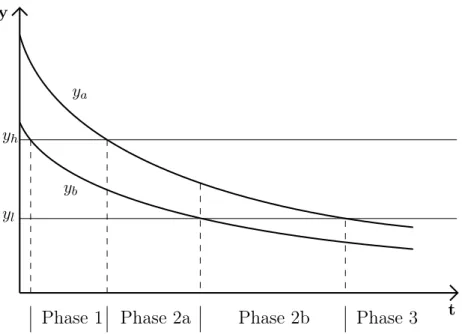
Bearing in mind that industry a’s good is purchased by richer consumers than industry b’s good, the dynamic development of the economy can be divided in the following way: first, none of the q-goods are being produced (phase 0). The profit-maximizing prices are both higher than the willingness to pay, even for the richest consumers with income yh. Then, the b-good is purchased by some fraction of the
consumers, while industry a’s good is not yet competitive due to its high marginal costs of production (phase 1). Next, both q−goods become competitive (phase 2). The following overview illustrates the different phases.
Phase 1 Some consumers can afford good b, while gooda is not yet competitive. ya(t)≥yh > yb(t)> yl
Aggregate demand for goodb is QDb (t) = 1 T Z yh yb(t) g(y)dy= α T(yh−yb(t)) (16) Phase 2a The richest households respectively buy one unit of thea-good, while a middle-class household buys the b-good. The poorest consumers fare better by buying neither of the goods (this is the case depicted in fig. 2).
yh > ya(t)> yb(t)> yl
If the proportion of consumers who buy one of the q-goods for the first time is small, aggregate demand approximates the replacement of all previous consumers’ endowment of one good. Demand for the twoq-goods then reads
QDa(t) = 1 T Z yh ya(t) g(y)dy= α T(yh−ya(t)) (17) QDb (t) = 1 T Z ya(t) yb(t) g(y)dy = α T(ya(t)−yb(t)) (18)
Phase 2b Market saturation. All consumers buy one unit of eitherq-good. During this phase, ceteris paribus, the market share of industry a’s good increases until it reaches 100%.
yh > ya(t)> yl≥yb(t)
Demand for the a-good is as in Phase 2a, while demand for the b-good be-comes QDb (t) = 1 T Z ya(t) yl g(y)dy = α T(ya(t)−yl) (19) Phase 3 Only good a is competitive. Consumers are sufficiently rich to value the difference in quality between the q-goods more than the corresponding difference in the prices.
yh > yl > ya(t)> yb(t)
Demand for gooda is maximal: QDa(t) = 1 T Z yh yl g(y)dy= α T(yh−yl) (20) Fig. 3depicts the phases, and the respectively corresponding relationships of critical incomes yb and ya. It becomes clear that not all phases must necessarily actually
occur. For instance, if the ya-curve is sufficiently far above the yb-curve, it may be
that the market is saturated with good b before good a becomes cheap enough for any consumer to buy it.
3.4
Results
In order to explore the dynamics of production and employment, it is appropriate to make some further assumptions regarding the industries’ technology, i.e. the parame-tersγj andAj. Specifically, we consider proportionally decreasing costs of production
in industry a and b. That is, the rates of technological progress in both industries are equal,γa=γb =γ, and the scale factors Aj differ: Aa< Ab.5
In the case considered here the profit-maximizing prices (15) become pa(t) = rβw1−βµ Aaeγt ; pb(t) = rβw1−βµ Abeγt (21) Production in the two phases can be calculated by plugging prices (21) in equa-tions (16-20).
5Without this assumption, theb-good would be redundant because no consumer would buy it at any time.
ya yb t y yh yl
Phase 1 Phase 2a Phase 2b Phase 3
Fig. 3: Technological change and the product cycle
When does the transition between different phases take place? Phase 1 begins when the richest households start buying the less expensive good b. The condition that must be fulfilled at the moment of transition is yb(t) =yh. Inserting eq. (11) for
yb and solving for t gives:
t1 = 1 γ ·ln µr1+βw1−βeδ yhAb(erT −1)·(eδ−1−1) (22) An analogous procedure yields the point in time when thea-good becomes com-petitive: t2a = 1 γ ·ln " µr1+βw1−β · eδ−1A a−Ab yhAaAb(erT −1)·(eδ−1−1) # (23) As figure 3illustrates, the length of the phases depends on the distance between the two curves representingyb and ya, respectively. If theyb-curve intersects the
hor-izontal yl line before theya-curve reachesyh, phase 2a will be missed out. According
to the definition of phase 2b, it starts when even the poorest consumer begins to buy one q-good. Therefore, we can state the condition that must be fulfilled at that moment as yb =yl. Using eq. (11) obtains
t2b = 1 γ ·ln µr1+βw1−β ylAb(erT −1)·(1−e−δ) (24) Phase 2b is terminated when qb is no longer competitive. This takes place when
ya=yl. Making use of eq. (13) gives
t3 = 1 γ ·ln " µr1+βw1−β · A a−Abe1−δ ylAaAb(erT −1)·(1−e1−δ) # (25)
Does technological progress have a detrimental effect on employment in this model? The answer is yes, from a critical point in time onwards, the labour-saving effect of technological progress more than compensates for the labour-augmenting effect of a higher demand that may result from price cuts. The reason for this un-ambiguous result is related to theorem 1 and equation (3). In the beginning, the price cuts that are caused by cost-reducing process innovations bring about higher demand. The relative size of these increases in demand shrinks, however, precisely because overall demand increases, i.e. demand becomes ever less elastic over time. When the elasticity approaches minus one, eventually a point is reached where both effects on labour demand are equally strong. From this moment onwards, technolog-ical progress lowers demand for labour.
The points in time when employment starts to decrease due to technological progress are different for the two q-goods. The elasticity of demand for the b-good from phases 2a and 2b (demand functions eq. (18) and eq. (19)) is clearly greater than minus one. This implies that either the critical moment is at t2a (i.e. when the
a-good becomes competitive, see eq. (23)), or before. Since the cross-price elasticity ηQ2,p1 is zero during phase 1, the condition that must be fulfilled at the moment when
technological progress starts to be detrimental to employment in the b-production is that the direct price elasticity equals -1 (see eq. (3)):
ηQb,pb = d dpb hα T(yh−yb(t)) i · pb Qb = −µr 1+βw1−βeδ−γt (erT −1)·(eδ−1)y hAb −µr1+βw1−βeδ−γt =−1
Solving this equation for t, we obtain t∗b = 1 γ ·ln 2r1+βµw1−βeδ yhAb(eδ−1)·(erT −1)
Building the derivative of t∗b with respect tow and T gives ∂t∗b ∂w = 1 γ · 1−β w >0; ∂t∗b ∂T = −1 γ · rerT erT −1 <0
Higher wages thus extend the period during which productivity has a positive impact on employment. The reason for this is that the number of consumers of the good is lower due to a higher price, which implies a higher elasticity. The level of employment must be lower than with low wages, however. The second result is that a longer economic life of the q-goods causes employment to reach its maximum earlier. The reason for this is simply that more consumers can afford the annual savings that are necessary to buy the q-good. The elasticity of demand decreases, and the point in time when productivity growth starts to have a detrimental effect on employment is reached earlier.
If this moment is before gooda becomes competitive (phase 2a), increasing pro-duction and productivity are accompanied by decreasing employment. The condition that must be fulfilled is
t∗b < t2a 1 γ ·ln 2r1+βµw1−βeδ yhAb(eδ−1)·(erT −1) < 1 γ ·ln " µr1+βw1−β · eδ−1Aa−Ab yhAaAb(erT −1)·(eδ−1−1) # A1 A2 < e−e 1−δ 2e−eδ−1
As is to be expected, the answer depends on the relationship between the productivity parametersAj, and on the relative preference of consumers regarding the twoq-goods,
expressed by the parameter δ. The lower the costs in theb-production relative to the a-production, and the less pronounced the consumers’ preference towards thea-good, the more likely it is that employment in the b-production will decrease before good a becomes competitive.
Goodbis special in that it is the first good that is ready for the market. Because of this, the cross-price elasticity with respect to pa is zero during the first phase,
so that only the price of good b must be considered (see corollary 1). In this view, phase 1 represents the one-industry case. In reality, there are more or less close substitutes, and the technology in the production of these substitutes is subject to changes as well, however. Therefore, finding the point in time when productivity growth has a detrimental effect on employment in the a-industry is somewhat more complicated, but also more interesting, since this case is meant to be representative of the continuum of industries that characterizes real-world economies.
In our two-industry case, productivity growth lowers the prices of bothq-goods, and the lower price of the respective substitute causes a further negative effect on production and employment (in addition to the decreasing direct elasticity of demand). As a consequence, the sum of the direct and the cross-price elastici-ties must equal minus one at the moment when employment has reached its peak: ηQa,pa(t∗a)+ηQa,pb(t∗a) =−1. Building the elasticities and solving for t yields
t∗a = 1 γ ln " 2r1+βw1−βµ A b−eδ−1Aa yhAaAb(erT −1)·(1−eδ−1) #
Again, this point in time depends positively on factor pricesr and w, and negatively on T. The first derivative with respect to δ is positive, which means that maximum employment in the a-industry is later if this good is less preferred relative to the b-good. Since this is accompanied by lower demand for good a throughout the entire product cycle, the relative change in demand that is caused by a decrease in the price pa is stronger and the employment effect is positive.
The results we derived for employment and the production of good a are meant to be representative of industries that face competition not only within the industry, but also from firms in other industries, due to the substitutability of the goods. In order to elaborate the effects most clearly, we assumed that the goods are close substitutes (only one of which may be consumed), but our basic findings do not hinge on this assumption, as is shown in section 2, where no assumptions regarding the degree of substitutability were made.
4
Structural change and regional employment
dis-parities
The model we described in the previous section provides a micro-foundation for the more general analysis of section 2. The point we made in an admittedly stylised framework is that the effects of technological progress on employment depend upon the elasticity of aggregate demand. The latter decreases as the product of the industry we look at advances in its product cycle, so that eventually the point is reached when price are accompanied by a slackening of demand. At the latest then, employment in the industry starts to decrease.
Our results may explain the large differences in the employment performance of various countries. In an econometric paper Möller (2001) found that in the passing of time the demand elasticity decreased in all three countries he studied, in the USA, in the UK, and in Germany. In the latter country the decrease was strongest and affected the economy especially during the early nineteen-seventies, in a phase of growing unemployment. Since then employment developed worse than in other comparable countries. This might be due to the specialisation of the country on manufacturing and especially on products of a relatively high quality. Often these products are not absolutely innovative. The German economy is highly competitive regarding relatively mature products, whose markets are characterised by low demand elasticities. The price for this specialisation may be low employment.
It is possible to reconcile the model presented here with the standard approach of macroeconomics developed by Layard et al. (1991) and their many followers. In that framework a price-setting function takes the role of the labour demand function. The corresponding wage-setting function represents the functional relationship between wages and unemployment, which may be based on efficiency wage or wage negotiation processes. Shifts of the price setting functions could be triggered by the theorem substantiated here. It should be noted that models of the Layard et al. -type are
based on monopolistic competition whereas our model relies on perfect competition. But this is of minor importance for the causal process studied here. At any rate one might add a wage setting curve to our model to reproduce the style of modern macroeconomics. In a framework of this kind different unemployment rates could be obtained.6
The comparison with modern macroeconomic approaches helps to clarify another point, namely the role of our assumption of fixed wages. If wages would adjust flexibly according to the regional scarcity of labour, the industry mix of the regions and the maturity of the corresponding products would have no effect on unemployment. This is excluded in the concept of the wage setting curve. According to this concept, which is compatible with many of the prevailing theories of unemployment like efficiency wages and union bargaining, a higher unemployment rate comes along with a lower wage rate. If we would allow for wages that are to some extent flexible, this would mitigate our results. Lower employment would translate into higher unemployment, which comes along with lower wages. The decrease of wages would lead to an increase in labour demand, which could not outweigh the initial impulse, however. In addition, the comparative-static results we derived suggest that the lower wage rate would only accelerate the process, so that wages would have to decline ever faster. In summary we claim that the specialisation of regions with respect to their industrial structure explains (to a large extent) interregional differences in the dynamics of unemployment. Our findings may help to explain why employment, and accordingly unemploy-ment differ greatly across regions within one country. The standard approach (Layard et al., 1991) emphasises the influence that institutions have on labour market out-come, and is thus silent regarding regional differences, since the institutional setting is usually the same for all regions within one country. Two more steps are required for our claim to hold: first, we argue that the industrial structure differs across regions, and that according to the results of our theoretical analysis, these differences are at the source of the employment dynamics. Second, we maintain that the development of employment is closely related to the regions’ performance regarding unemployment (see Blanchard and Katz (1992) and Elhorst (2003)).
The production of many goods is clustered in relatively small areas. A new debate revealed a characteristic asymmetry. Agglomeration forces are visible for 6Under monopolistic competition the firm is operating on the elastic part of the firm-individual demand function. For an individual firm the actions of all other firms are given. If all firms would set their prices symmetrically, however, the consumers’ ability to react to price changes would be reduced. Therefore, the elasticity of aggregate demand is always lower than the elasticity one specific firm faces. Accordingly, it may well be that aggregate demand is inelastic, even under monopolistic competition.
productivity, but not for employment (see Cingano and Schivardi (2004) and Combes et al. (2004)). This means that productivity grows faster in large agglomerations but employment in the rural country. This striking discrepancy can easily be understood by the results derived in this paper.
Although there are only a few regions that are as lopsided as, for instance, the automobile industry in Detroit, or high-tech businesses in Silicon Valley, it is cer-tainly the case that each region has its specific mix of industries, which is shaped by economic as well as historical, geographical and other factors. Our model suggests that the specific industrial structure that characterises a region determines how em-ployment evolves over time. Regions that exhibit a relatively large share of ”young“ industries, which produce goods that are at the beginning of their product cycle, fare better in terms of employment than other regions. Notice that our argument is not restricted to industries in decline, such as mining and heavy industry, which would be trivial. Regions with a high number of silicon chip producers may well soon encounter the same sort of employment problems as regions with a large share of automobile industry are experiencing now. Our theoretical analysis suggests that the rise and decline of employment is inherent in any industry, and thus inevitable.
Coming back to wages, it should be emphasised that there is a regional equiva-lent to the macroeconomic concept of the wage-setting curve, called the ”wage curve“. According to this concept, which was proposed by Blanchflower and Oswald, the em-pirical elasticity of wages with respect to regional unemployment is -0.1.7 Therefore, regional wages are far from being completely flexible. Only fully flexible wages would be able to neutralise our results, however.
5
Conclusion
The model presented in this study captures an important, but widely ignored property of product markets, namely a decreasing elasticity of aggregate demand over the product cycle (see Möller, 2001). We are able to trace back the decrease in the price elasticity to individual utility maximisation.
We explain the development of employment by the interaction of supply and demand forces. The effects of productivity gains may vary according to the elasticity of demand on product markets. Since we found forces which shift this elasticity 7The absolute size of the effect is a point of debate. Arguably, it might be smaller in absolute terms than -0.1. This is the result of a meta-study that corrects for the ’publication bias’ (Nijkamp and Poot, 2005). In the German case, many studies showed that the coefficient is smaller than the international average, see Blien (2001) and Baltagi and Blien (1998).
from higher to lower values (in absolute terms), product cycles are related to their microeconomic basis. The employment of nations, regions, cities or industries is affected by the position of their leading products within their respective product cycle.
As to policy conclusions the results obtained are quite striking. In the first phase of development – after the introduction of an innovative product – measures taken to assist the infant industry have positive employment effects. These grow even larger when the industry matures and gains more and more weight in the region or nation it is located. During this time all the measures assisting the ascending industry increase employment. But then, unknown to the actors in the respective region (or nation), a turning point is reached. Now the same measures have detrimental effects on employment and therefore adverse effects on the whole region (or nation). Thus, the same measure might have very different effects with respect to space and time.
References
Appelbaum E. and Schettkat R. (1993): “Employment Developments in Industrialized Economies: Explaining Common and Diverging Trends.” Discussion Paper 93-313, Wissenschaftszentrum Berlin für Sozialforschung.
Baltagi B.H. and Blien U. (1998): “The German Wage Curve: Evidence from the IAB Employment Sample.” Economics Letters, 61, 135–142.
Blanchard O.J. and Katz L.F. (1992): “Regional Evolutions.” Brookings Papers on Economic Activity, 1, 1–75.
Blanchflower D.G. and Oswald A.J. (2005): “The Wage Curve Reloaded.” Working Paper 11338, NBER.
Blien U. (2001): Arbeitslosigkeit und Entlohnung auf regionalen Arbeitsmärk-ten: Theoretische Analyse, ökonometrische Methode, empirische Evidenz und wirtschaftspolitische Schlussfolgerungen für die Bundesrepublik Deutschland. Heidelberg: Physica-Verlag.
Cavelaars P. (2005): “Has the Tradeoff Between Productivity Gains and Job Growth Disappeared?” Kyklos, 58, 45–64.
Cingano F. and Schivardi F. (2004): “Identifying the Sources of Local Productivity Growth.” Journal of the European Economic Association, 2, 720–742.
Combes P.P., Magnac T. and Robin J.M. (2004): “The Dynamics of Local Employ-ment in France.” Journal of Urban Economics, 56, 217–243.
Elhorst P.J. (2003): “The Mystery of Regional Unemployment Differentials: Theo-retical and Empirical Explanations.” Journal of Economic Surveys, 17, 709–748. Freeman R.B. (2001): “Single-peaked versus Diversified Capitalism: The Relation Between Economic Institutions and Outcomes.” In Advances in Macroeconomic Theory, J. Drèze, ed. Basingstoke: Palgrave, 139–170.
Layard R., Nickell S. and Jackman R. (1991): Unemployment: Macroeconomic Per-formance and the Labour Market. Oxford: Oxford University Press.
Möller J. (2001): “Income and Price Elasticities in Different Sectors of the Economy: An Analysis of Structural Change for Germany, the UK and the USA.” In The Growth of Service Industries: The Paradox of Exploding Costs and Persistent Demand, T. ten Raa and R. Schettkat, eds. Cheltenham: Edward Elgar, 167– 208.
Nijkamp P. and Poot J. (2005): “The Last Word on the Wage Curve?” Journal of Economic Surveys, 19, 421–450.
Südekum J. (2005): “Increasing Returns and Spatial Unemployment Disparities.” Papers in Regional Science, 84, 159–181.
IABDiscussionPaper No. 6/2006
In dieser Reihe sind zuletzt erschienen
Recently published
No. Author(s) Title Date
1/2004 Bauer, Th. K.,
Bender, St., Bonin, H.
Dismissal Protection and Worker Flows in Small Establishments
7/2004
2/2004 Achatz, J.,
Gartner, H., Glück, T.
Bonus oder Bias? Mechanismen geschlechts-spezifischer Entlohnung
7/2004
3/2004 Andrews, M.,
Schank, Th., Upward, R.
Practical estimation methods for linked employer-employee data
8/2004
4/2004 Brixy, U.,
Kohaut, S., Schnabel; C.
Do newly founded firms pay lower wages? First evidence from Germany
9/2004
5/2004 Kölling, A,
Rässler, S.
Editing and multiply imputing German estab-lishment panel data to estimate stochastic production frontier models
10/2004
6/2004 Stephan, G, Gerlach, K.
Collective Contracts, Wages and Wage Dispersion in a Multi-Level Model
10/2004
7/2004 Gartner, H. Stephan, G.
How Collective Contracts and Works Councils Reduce the Gender Wage Gap
12/2004
1/2005 Blien, U., Suedekum, J.
Local Economic Structure and Industry Development in Germany, 1993-2001
1/2005
2/2005 Brixy, U., Kohaut, S., Schnabel, C.
How fast do newly founded firms mature? Empirical analyses on job quality in start-ups
1/2005
3/2005 Lechner, M.,
Miquel, R., Wunsch, C.
Long-Run Effects of Public Sector Sponsored Training in West Germany
1/2005
4/2005 Hinz, Th.,
Gartner, H.
Lohnunterschiede zwischen Frauen und Männern in Branchen, Berufen und Betrieben
2/2005
5/2005 Gartner, H., Rässler, S.
Analyzing the Changing Gender Wage Gap based on Multiply Imputed Right Censored Wages
IABDiscussionPaper No. 6/2006
6/2005 Alda, H., Bender, S., Gartner, H.
The linked employer-employee dataset of the IAB (LIAB)
3/2005
7/2005 Haas, A., Rothe, Th.
Labour market dynamics from a regional perspective
The multi-account system
4/2005
8/2005 Caliendo, M., Hujer, R., Thomsen, S.L.
Identifying Effect Heterogeneity to Improve the Efficiency of Job Creation Schemes in Germany
4/2005
9/2005 Gerlach, K., Stephan, G.
Wage Distributions by Wage-Setting Regime 4/2005 10/2005 Gerlach, K.,
Stephan, G.
Individual Tenure and Collective Contracts 4/2005 11/2005 Blien, U.,
Hirschenauer, F.
Formula allocation: The regional allocation of budgetary funds for measures of active labour market policy in Germany
4/2005
12/2005 Alda, H.,
Allaart, P., Bellmann, L.
Churning and institutions – Dutch and German establishments compared with micro-level data
5/2005
13/2005 Caliendo, M.,
Hujer, R., Thomsen, St.
Individual Employment Effects of Job Creation Schemes in Germany with Respect to Sectoral Heterogeneity
5/2005
14/2005 Lechner, M.;
Miquel, R., Wunsch, C.
The Curse and Blessing of Training the Unemployed in a Changing Economy
- The Case of East Germany after Unification
6/2005
15/2005 Jensen, U.; Rässler, S.
Where have all the data gone? Stochastic production frontiers with multiply imputed German establishment data
7/2005
16/2005 Schnabel, C.; Zagelmeyer, S.; Kohaut, S.
Collective bargaining structure and ist deter-minants: An empirical analysis with British and German establishment data
8/2005
17/2005 Koch, S.; Stephan, G.; Walwei, U.
Workfare: Möglichkeiten und Grenzen 8/2005
18/2005 Alda, H.; Bellmann, L.; Gartner, H.
Wage Structure and Labour Mobility in the West German Private Sector 1993-2000
8/2005
19/2005 Eichhorst, W.; Konle-Seidl, R.
The Interaction of Labor Market Regulation and Labor Market Policies in Welfare State Reform
IABDiscussionPaper No. 6/2006
20/2005 Gerlach, K.; Stephan, G.
Tarifverträge und betriebliche Entlohnungs-strukturen
11/2005
21/2005 Fitzenberger, B.; Speckes-ser, S.
Employment Effects of the Provision of Specific Professional Skills and Techniques in Germany
11/2005
22/2005 Ludsteck, J., Jacobebbing-haus, P.
Strike Activity and Centralisation in Wage Setting 12/2005 1/2006 Gerlach, K., Levine, D., Stephan, G., Struck, O.
The Acceptability of Layoffs and Pay Cuts: Comparing North America with Germany
1/2006
2/2006 Ludsteck, J. Employment Effects of Centralization in Wage
Setting in a Median Voter Model
2/2006
3/2006 Gaggermeier, Ch.
Pension and Children: Pareto Improvement with Heterogeneous Preferences
2/2006
4/2006 Binder, J., Schwengler, B.
Korrekturverfahren zur Berechnung der Einkommen über der Beitragsbemessungs-grenze
3/2006
5/2006 Brixy, U., Grotz, R.
Regional Patterns and Determinants of New Firm Formation and Survival in Western Germany
IABDiscussionPaper No. 6/2006
Impressum
IABDiscussionPaper No. 6 / 2006
Herausgeber
Institut für Arbeitsmarkt- und Berufsforschung der Bundesagentur für Arbeit
Weddigenstr. 20-22 D-90478 Nürnberg Redaktion
Regina Stoll, Jutta Palm-Nowak Technische Herstellung Jutta Sebald
Rechte
Nachdruck – auch auszugsweise – nur mit Genehmigung des IAB gestattet
Bezugsmöglichkeit
Volltext-Download dieses DiscussionPaper unter:
http://doku.iab.de/discussionpapers/2006/dp0606.pdf
IAB im Internet
http://www.iab.de
Rückfragen zum Inhalt an Uwe Blien, Tel. 0911/179-3035, oder e-Mail: uwe.blien@iab.de