Energy Procedia 45 ( 2014 ) 1027 – 1036
1876-6102 © 2013 The Authors. Published by Elsevier Ltd.
Selection and peer-review under responsibility of ATI NAZIONALE doi: 10.1016/j.egypro.2014.01.108
ScienceDirect
68th Conference of the Italian Thermal Machines Engineering Association, ATI2013
Hierarchical 1D/3D approach for the development of a turbulent
combustion model applied to a VVA turbocharged engine.
Part II: combustion model
Vincenzo De Bellis
a*
, Elena Severi
b, Stefano Fontanesi
b, Fabio Bozza
aa Industrial Engineering Department, Mechanic and Energetic Section, University of Naples “Federico II”, Naples, Italy.
b Department of Engineering “Enzo Ferrari”, University of Modena and Reggio Emilia, Modena, Italy
Abstract
As discussed in the part I of this paper, 3D models represent a useful tool for a detailed description of the mean and turbulent flow fields inside the engine cylinder. 3D results are utilized to develop and validate a 0D phenomenological turbulence model, sensitive to the variation of operative parameters such as valve phasing, valve lift, engine speed, etc.
In part II of this paper, a 0D phenomenological combustion model is presented, as well. It is based on a fractal description of the flame front and is able to sense each of the fuel properties, the operating conditions (air-to-fuel ratio, spark advance, boost level) and the combustion chamber geometry. In addition, it is capable to properly handle different turbulence levels predicted by means of the turbulence model presented in the part I.
The turbulence and combustion models are included, through user routines, in the commercial software GT-Power™. With reference to a small twin-cylinder VVA turbocharged engine, the turbulence/combustion model, once properly tuned, is finally used to calculate in-cylinder pressure traces, rate of heat release and overall engine performance at full load operations and brake specific fuel consumption at part load, as well. An excellent agreement between numerical forecasts and experimental evidence is obtained.
© 2013 The Authors. Published by Elsevier Ltd.
Selection and peer-review under responsibility of ATI NAZIONALE.
Keywords: internal combustion engine; turbulence; combustion; 0D/3D modeling.
* Corresponding author. Tel.: +39-081-7683264; fax: +39-081-2394165. E-mail address: vincenzo.debellis@unina.it
© 2013 The Authors. Published by Elsevier Ltd.
Nomenclature
A Area
cenh1 Karlovitz related burning rate enhancement factor cenh2 Mean flow related burning rate enhancement factor
ctrans Tuning constant of the transition time from laminar to turbulent combustion cwc Burned gas fraction at wall combustion start
cwrk Tuning constant of the flame front maximum wrinkling length scale D Turbulent kinetic energy dissipation rate
D3 Flame front fractal dimension k Turbulence kinetic energy
Ka Karlovitz number
lk Kolmogorov length scale LI Integral length scale
Lmax Length scale of the maximum flame front wrinkling
Lmin Length scale of the minimum flame front wrinkling
m Mass
q Wiebe function
r0 Initial flame front radius Ret Turbulence Reynolds number u’ In-cylinder turbulence fluctuation
Uflow In-cylinder mean flow velocity SL Laminar flame speed
ST Turbulent flame speed t Time, characteristic time scale
tstart Combustion start time
ttrans Transition time from laminar to turbulent combustion twc Transition time from turbulent to wall combustion w1, w2 Weight factors of the burning rate
Greeks
Gf Flame front thickness
H Specific turbulent kinetic energy dissipation rate
U Density
W Wall combustion characteristic time X Kinematic viscosity
Zwr Non-dimensional flame-wrinkling rate
Subscripts
b Related to burned gas
u Referred to the unburned gas Acronyms
BDC, TDC Bottom - Top dead center BSFC Brake specific fuel consumption CFD Computational fluid dynamic EIVC Early intake valve closure ICE Internal combustion engine IMEP Indicated mean effective pressure SI Spark ignition
1.Introduction
As evidenced in the first part of the paper, the synergic use of different simulation tools can relevantly contribute to the development and optimization of advanced control strategies for internal combustion engines.
The above statement is particularly true for last generation units, both spark-ignited and compression-ignited, in view of the mutual interaction between many complex sub-systems and technologies, such as Variable Valve Actuation (VVA), turbocharging and direct injection.
Numerical analyses can in fact drastically reduce the number of experiments and prototypes during the early design stages, as well as contribute to the investigation of a wide number of control strategies during the engine calibration phase, providing the designers a “virtual calibration” environment.
Particularly, many issues related to the design (comparison of different components and turbochargers) and calibration (identification of proper valve actuation, EGR and turbocharger strategy at part and full load, as well) of a modern spark ignition engine can be successfully accomplished by means of 1D codes. However, the design of some sub-components (for instance, combustion chamber shape, air filter design, etc.) is demanded to the more refined 3D CFD tools which, on the other hand, require higher computational time.
Nowadays, many automotive manufactures make an extensive use of 1D simulation codes, which are more easily able to completely describe the engine behavior starting from the intake mouth up to the exhaust tailpipe.
Since many years, two-zone quasi-dimensional models have been proposed in the current literature [1,2,3] and some of them are usually employed in a number of proprietary or commercial one-dimensional codes. They are based on different theoretical approaches, trying to describe the flame development inside a turbulent flow field.
A popular theory is the entrainment of turbulent eddies in the flame front. These eddies burn inwards from peripheral ignition sites to be consumed in a characteristic time with the laminar burning speed. The entrainment velocity is given by an algebraic equation from the flamelet modeling relations. The entrainment theory is rather a mathematical modeling that agrees with the S-shaped burned mass fraction, which is observed in experiments [4,5]. Entrainment combustion mechanisms have not been experimentally observed in real premixed flames. Nevertheless, the mathematical efficiency of this theory makes it a popular choice in 0D modeling .
Among the different approaches, the “fractal” combustion model appears to be the one which better describes the turbulent flame propagation phenomenon inside an internal combustion engine [1,2,6,7,8]. It is based on the hypothesis that aerodynamic turbulence enhances the burn rate by increasing the surface of the flame front with respect the laminar extent and does not alter significantly the inner flame structure. All turbulent length scales are assumed to be larger than the flame front thickness (flame is in the so called “wrinkled flamelet” regime).
The combustion model presented in this work is integrated with the turbulence one, shown and validated in the part I. Firstly, the combustion model is described in detail. Its consistency is demonstrated by verifying that the computed combustion regime really belongs to the “wrinkled flamelets”. Then, the model is applied to the simulation of a small twin-cylinder VVA turbocharged engine described in the part I at full load operations. The provided results are compared with the experimental data both in terms of overall performance parameters (power/torque, air mass flow rate, BSFC and turbocharger speed) and in-cylinder pressure cycles. Finally, model reliability is demonstrated at part-load operation, as well.
2.Combustion model description
An extensive description of the fractal model is already reported in [9,10,11,12,13]. In the wrinkled-flamelet regime of combustion occurring inside an ICE [1,2,14], the burning rate can be expressed as:
b T u T L u L L L dm A A S A S dt U U A § · ¨ ¸ © ¹ (1)
ȡu being the unburned gas density. Equation (1) puts into evidence that the burning rate is mainly increased by the
wrinkling of the flame surface AT determined by the turbulent flow field, with respect to the corresponding smooth
laminar flame speed, SL, which is a function of the fuel type, air/fuel ratio and residual gas fraction. The employed
correlation also accounts for flame stretch mainly occurring during the first phase of burning process [15]. Under this schematization, moreover, the burning rate can be easily computed once the increase in flame area has been established. Basing on the concepts of the fractal geometry, the latter can be easily expressed as a function of a minimum and maximum flame wrinkling scales, Lmin-Lmax, and to its fractal dimension D3:
3 2 max min D T L L A A L § · ¨ ¸ © ¹ (2)
Lmin is assumed equal to the Kolmogorov length scale, lk, which, under the hypothesis of isotropic turbulence,
follows the expression:
3 4 Re I k t L l Re ' I t u u L X (3)
Xu being the kinematic viscosity of the unburned mixture. The turbulent intensity u’ and the integral length scale LI
are given by the K-k model described in Part I. Lmax, indeed, representing the dimension of the maximum flame front wrinkling, is related to some characteristic dimension the flame front, such as the flame radius or the square root of the laminar surface. In the present version of the model, the latter choice is followed, and the Lmax is computed according to:
max wrk L
L c A (4)
cwrk being a tuning constant. The D3 dimension only depends on the ratio between the turbulence intensity u’ and the laminar flame speed SL, reported in [14].
The above described fractal model is really valid for a fully developed and freely expanding turbulent flame. During both early flame development and combustion completion, a different approach is required. Initial flame development is in fact dominated by the kernel formation phase; its duration is calculated by an Arrhenius-like formulation, also accounting for residual fraction contents. At the end of the kernel formation time, the computation of the combustion process starts with a stable and spherically-shaped smooth flame, of radius r0. Flame wrinkling
process also starts at a rate, Ȧwr, which increases with the normalized elapsed time after the combustion start.
start wr trans t t t Z (5)
The transition time, ttrans, in the above equation is hence considered as a time scale during which the flame front
evolves from an initial smooth surface – corresponding to a laminar-like combustion – to a fully developed turbulent wrinkled flame. The transition time is assumed proportional to a characteristic turbulent time scale, calculated as:
trans trans k
t c
D (6)
ctrans being a tuning constant, while k and D are the turbulence kinetic energy and its dissipation rate, (see part I).
Flame wrinkling rate Ȧwr affects the calculation of the maximum fractal dimension of the flame, according to:
3,max 2.00 1 1 2.35 1 1 wr
q being the well-known Wiebe function. In this way, the D3 expression in [14] is redefined as: 3,max 3 ' 2.00 ' L L D u S D u S (8)
With this formulation, the first phase of the combustion process (w1~ 0) is characterized by a fractal dimension close to 2.00, corresponding to an initial laminar burning process.
A different combustion rate is also specified when the flame front reaches the combustion chamber walls (wall combustion phase). Wall-combustion burning rate is simply described by an exponential decay, as follows:
b b wall combustion dm m m dt W § · ¨ ¸ © ¹ (9)
IJ EHLQJ WKH FKDUDFWHULVWLF WLPH VFDOH of the above process. The overall burning rate is consequently defined as a weighted mean of the two described combustion rates:
2 1 2
b b b
fractals wall combustion
dm dm dm w w dt dt dt § · § · § · ¨ ¸ ¨ ¸ ¨ ¸ © ¹ © ¹ © ¹ (10)
The switch between the two combustion modes gradually starts when a threshold value, cwc, of the burned gas
fraction is reached (transition time, twc). At this time, the characteristic time scale in eq. (9) is computed assuming
that the wall combustion burning rate equals the one derived from the fractal model, eq. (1), hence:
, , b t wc u T L t wc m m A S W U 2 , b b t wc m m w m m (11) 7KHDERYHIJYDOXHLVWKHQNHSWIL[HGGXULQJWKHVXEVHTXHQWZDOOFRPEXVWLRQSURFHVV7KHZHLJKWIDFWRUw2 indeedincreases with time, depending on the instantaneous unburned mass (m - mb), compared to the one occurring at the
transition time, twc. In this way, a smooth transition between the two modes is easily obtained. It is important to note
that the above schematization of the wall combustion, based on the analysis of typical heat release data, does not include any additional tuning constant. Finally, two corrections are introduced in the turbulent flame front area calculation:
3 2 max 1 2 1 min 1 1 1 D flow T enh enh L T U L A c Ka c w A L S ª º § · ª º ¨ ¸ ¬ ¼« » © ¹ ¬ ¼ (12)Ka in the above equation is the Karlovitz number which is computed as: 2 f u f k L Ka l S G X G § · ¨ ¸ ¨ ¸ © ¹ (13)
Gf being the flame front thickness. The first correction accounts for the enhanced species mixing in the flame front
and is activated only when the Ka > 1 inequality verifies. In this case, in fact, the flame thickness is larger than the Kolmogorov turbulence micro-scale and turbulent eddies are able to enhance the burning speed. This verifies in the case of high turbulence levels (high engine speed) or slow laminar flame speed (large amount of trapped EGR, very lean or very reach mixtures, for instance). Simultaneously, at very high Karlovitz numbers, the flame deformation
determined by the turbulent flow field can be so intense to produce a multiple connected flame front, with “islands” of unburned mixture trapped within the burned gas zone. This is mainly due to the increased convective action of the turbulent field, that can stretch and break the flame, determining pockets of unburned mixture within the burned gas zone. As a consequence, the reaction surface and the burning speed increase.
The second correction term is justified by the possibility of a flame front distortion, that may occur when an intense mean flow is present in the cylinder. Each term is weighted by additional tuning constants, cenh1 and cenh2.
3.Engine model description
The engine model is developed in the GT-Power commercial software, based on a 1D description of the flow inside the intake and exhaust pipes. The combustion process and the turbulence phenomenon are described using the previously described sub-models; they are introduced in GT-Power through “user routines”.
The VVA system that equips the tested engine allows for different strategies such as the LIVO (Late Intake Valve Opening), the EIVC (Early Intake Valve Closure), a combination of the previous ones and a multi-lift strategy. To simplify the engine calibration issue, among the available strategies, the EIVC is only employed.
Thanks to a 1D model of the valve actuation system developed in the AmesimTM, a “database” of valve lift profiles for various engine speeds as well as closure angle is computed. The latter is inquired by a GT-Power “user routine” to evaluate by interpolation the actual lift profile, depending on the engine operating conditions.
4.Combustion model results
4.1.Preliminary 3D-CFD results
As described in the part I of the paper, results from CFD-3D full-cycle simulations are preliminarily used in order to calibrate the K-k turbulence model, and therefore to provide a more robust physical background for the combustion analyses.
In fact, in order to better account for the effects of massively different valve actuation strategies on the establishment and subsequent decay of organized flow structures within the cylinder, a set of calculations is performed under motored conditions covering both high and low engine speeds and valve lift typical of full and part load operations (labeled FL and PL, respectively, in Figure 1 and 2).
5100FL 2500FL 3000PL 2000PL
5100FL 2500FL 3000PL 2000PL
Figure 2. Normalized turbulent intensity fields @720 CAD
Results from this set of 3D simulations are here shortly recalled for the sake of brevity. Two main considerations can be deduced:
x the flow structures within the cylinder are strongly influenced by the valve actuation strategy, in both intensity and spatial distribution, as highlighted in Figure 1 that depicts the BDC turbulent intensity field in a cross plane that includes both intake and exhaust valve axes.
x the differences that arise during the scavenging process, although partly dampened during the compression stroke, are still present close to firing TDC, as shown in Figure 2. In particular, EIVC cases, typical of part-load operation, determine a longer time available for turbulence decay. As a consequence, lower maximum levels are reached in cases 3000PL and 2000PL. Valve strategy is hence expected to also affect burning speed.
4.2.1D combustion results
The operating parameters given as an input to the GT-Power engine model are the intake valve closure, the A/F ratio and the spark advance. Since information about the experimental turbine waste-gate valve opening are not available, the latter have to be indirectly evaluated using a PID controller and a target experimental datum, like the boost level, the mass flow rate or the turbocharger speed. The usage of the experimental boost level may introduce some inaccuracies in the simulations, since at low-speed/full-load the compressor operates in close-to-surge map region, where iso-speed slope are very reduced. Consequently, the map-derived mass flow rate cannot be precisely identified. On the other hand, the experimental mass flow rate or the turbocharger speed are usually affected by higher uncertainties. For this reason, an alternative strategy is proposed, aiming to identify the waste-gate opening realizing the experimental pressure level at the firing TDC for the cylinder #2. This level is in fact representative of the actual in-cylinder filling conditions since, at full-load, the combustion process, to avoid knocking, always begins after the TDC. The proposed strategy provided the best agreement with experimental data.
Table 1. Combustion model tuning constants
cwrk 0.5 ctrans 0.4 cwc 0.8 cenh1 0.5 cenh2 0.1
Results shown in Figure 3 are obtained after the tuning of the combustion model parameters (Table 1). They are kept constant for each analyzed operating condition. In particular, the Figures show the numerical/experimental comparison in terms of power, torque, air mass flow rate, BSFC and turbocharger speed. The agreement of the engine overall performance is satisfactory with the exception of the higher engine speeds. This is probably due to uncertainties in the Amesim-computed lift profiles, affecting the volumetric efficiency and the pumping work. In addition, due to the two-cylinder arrangement, large mass flow rate and pressure ratio oscillations are expected. Engine-turbocharger matching is hence a critical issue for this engine, since a strongly unsteady operation is expected for the turbocharger. This may also affect BSFC predictions at higher speeds.
Figure 3. Engine performance at full load. 1D model and experimental data comparison
Figure 4. Borghi Diagram
In order to verify that model results are consistent with the theoretical hypotheses that justify its formulation, the combustion regime establishing at different engine speeds is analyzed. This can be accomplished looking at two typical dimensionless parameters extracted from the simulations, namely the ratio between the integral length scale and the flame thickness, LI / įf , and the ratio between the turbulent intensity and the laminar flame speed, u’ / SL. These parameters are reported on the well-known Borghi Diagram in Figure 4, identifying the different combustion regimes occurring at different Reynolds, Karlovitz and Damkholer numbers, [16]. It is verified that, at each speed-load condition, the instantaneous trajectory on the Borghi plane always belongs to the wrinkled-flamelets regime, with the exception of the highest speed, where a local Ka > 1 value may occur at the beginning of the combustion process. At spark time, in fact, u’ is still high, while SL is reduced, due to intense flame stretch at small flame radius. Correction in eq. (12) roughly takes into account the above phenomena.
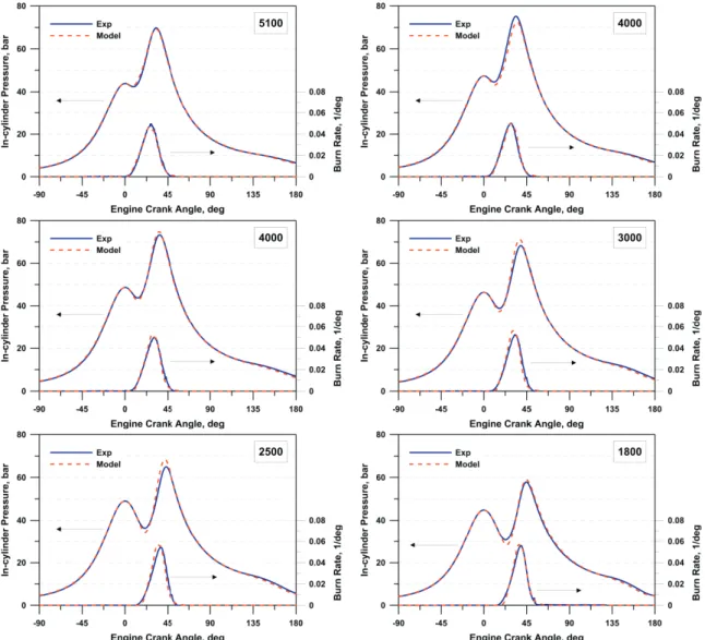
Figure 5. Numerical/Experimental comparison of in-cylinder pressure cycle and burn rate
Figure 5 shows the experimental/numerical comparison of pressure cycles and burn rates at 5100, 4400, 4000. 3000, 2500 and 1800 rpm during the compression and combustion/expansion phases. Especially at low engine speeds, the spark timing occurs late after the TDC, determining the displayed double-peak pressure cycles; this choice, although hardly penalizing IMEP and BSFC, is necessary to avoid knocking occurrence. Despite the above non-conventional operating conditions, the accuracy of the in-cylinder pressure cycle prediction is very high. Burn rates are also very well predicted, and the model properly describes the initial and final combustion evolution.
In order to test the reliability of the proposed model, further calculations are carried out at part load, for two different engine speeds. In particular, the BSFC is evaluated by specifying the experimentally actuated combustion center (MFB50%) and intake valve strategy. In Figure 6, the computed results are compared with the experimental ones, and a very satisfactory agreement can be observed, especially at 3000 rpm. It isn’t worthless to emphasize that tuning constants in turbulence and combustion models have been kept unchanged in each operating condition. 5.Conclusions
In the part II of this paper, a phenomenological 0D model for the description of the combustion process occurring in a spark ignition ICE is presented. It describes the flame front as a thin surface which separates burned and unburned gases and is corrugated by the turbulence vortices according to the fractal geometry theory. Proper corrections for the description of the early flame propagation and for the wall combustion phase are introduced. The fractal combustion model is coupled to the K-k turbulence model, presented in the part I of the paper, and calibrated against 3D-CFD simulations. The models are here employed to analyze a small twin-cylinders VVA turbocharged engine at full and part-load operation, as well. The engine behavior is very well predicted, without requiring a case-depending tuning, in terms of both overall performance, in-cylinder pressure cycles and burning rates. A very good agreement is also showed on fuel consumption forecasts at part-load.
Overall results discussed in Part I and II demonstrate how the proposed hierarchical 1D/3D approach can be very helpful for the development of consistent and accurate, although computationally inexpensive, models, which can be easily coupled to optimization codes, for the definition of optimal control strategies of modern SI engines.
References
[1] Matthews RD, Chin YW. A Fractal- Based SI Engine Model: Comparisons of Predictions with Experimental Data. SAE paper 910075, 1991. [2] Poulos SG, Heywood JB. The Effect of Chamber Geometry on Spark-Ignition Engine Combustion. SAE paper 830334, 1983.
[3] Bozza F, Gimelli A, Senatore A, Caraceni A. A Theoretical Comparison of Various VVA Systems for Performance and Emission Improvements of SI Engines. SAE Paper 2001- 01-0671, 2001, also in Variable Valve Actuation 2001, SAE SP-1599, ISBN 0-7680-0746-1. [4] Verhelst S, Sheppard CGW. Multi-zone thermodynamic modelling of spark-ignition engine combustion – An overview, Energy Conversion and Management. vol. 50, no. 5, pp. 1326–1335, May 2009, doi: 10.1016/j.enconman.2009.01.002.
[5] Rakopoulos CD, Michos CN, Giakoumis EG. Thermodynamic Analysis of SI Engine Operation on Variable Composition Biogas-Hydrogen Blends Using a Quasi-Dimensional, Multi-Zone Combustion Model. SAE paper 2009-01-0931, 2009, doi:10/4271/2009-01-0931.
[6] Franke C, Wirth A, Peters N. New Aspects of the Fractal Behaviour of Turbulent Flames. 23 Symp. (Int.) on Combustion, Orleans, 1990. [7] Gatowsky JA, Heywood JB. Flame Photographs in a Spark-Ignition Engine. Combustion and Flame, 56 pp. 71-81, 1984.
[8] Gouldin FC. An application of Fractals to Modeling Premixed Turbulent Flames. Sibley School of Mech. And Aerospace Eng., 1986. [9] Bozza F, Gimelli A, Merola SS, Vaglieco BM. Validation of A Fractal Combustion Model through Flame Imaging. SAE 2005 Transaction,
Journal of Engines - section 3, vol. 114-3, pp. 973-987, ISBN 0- 7680-1689-4, 2006.
[10]Onorati A, Ferrari G, Montenegro G, Caraceni A, Pallotti P. Prediction of S.I. Engine Emissions During An ECE Driving Cycle Via Integrated Thermo- Fluid Dynamic Simulation. SAE paper 2004-01-1001, SAE World Congress, Detroit, March 2004.
[11]Baratta M, Catania AE, Spessa E, Vassallo A. Development of an Improved Fractal Model for the Simulation of Turbulent Flame Propagation in SI Engines. ICE 2005, SAE paper 2005-24-082.
[12]Fontana G, Galloni E, Palmaccio R, Torella E. Numerical Analysis of a Small Turbo-Charged Spark-Ignition Engine. ICES 2006- 1336, ASME/ICE Spring Technical Conference 2006, Aachen.
[13]Bozza F, Gimelli A, Russo F, Torella E, Strazzullo L, Mastrangelo G. Application of a Quasi-Dimensional Combustion Model to the Development of a High-EGR VVT SI Engine. 7th Int. Conf. ICE05 2005. Capri (NA) - Italy. ISBN Number: 88-900399-2-2.
[14]North GL, Santavicca DA. The Fractal Nature of Premixed Turbulent Flames. Combustion Science and Technology, 1990.
[15]Bradley D, Lau AKC, Lawes M. Flame Stretch Rate as a Determinant of Turbulent Burning Velocity. Phil. Trans. R. Soc. Lond. A 1992 338, 359-387, doi: 10.1098/rsta.1992.0012.
[16]Lipatnikiv AN, Chomiak J. Turbulent Flame Speed and Thickness: Phenomenology, Evaluation and Application in Multidimensional Simulations. Progress in Energy and Combustion Science, 28, pp. 1-74, 2002.