Supervised machine learning of fullcube hyperspectral data

(1)

Supervised machine learning of

fullcube hyperspectral data

Extremely randomized trees for classification of tree species

Master Thesis

to obtain the degree "Master of Science (MSc)"

at the Department of Geoinformatics, University of Salzburg.

Supervisor: Dr. Nicole Pinnel

German Aerospace Center (DLR)

Author: Yannic Timothy Fetik

(2)

List of Figures

1 Study Area . . . 4

2 Height zones . . . 5

3 Tree species according to inventory . . . 5

4 Tree species mixture . . . 6

5 Coordination calculation for forest inventory pixels . . . 7

6 Sampling locations . . . 8

7 Calculated tree density for the northern part . . . 14

8 Canopy Height Model calculation . . . 14

9 Satellite image overlayed with CHM . . . 15

10 Workflow of single processing steps . . . 20

11 Confusion matrix for validation of previous study (Pixels) . . . . 22

12 Diagram visualising BRDF problems . . . 24

13 Diagram visualising BRDF problems . . . 25

14 Geometric and volume scattering . . . 25

15 Mosaic of Northern HySpex data . . . 26

16 Mean spectrum of species before and after Savitzky-Golay filter . 28 17 Mean tree species spectrum after Brightness Normalization . . . 29

18 Outliers detected by Isolation Forest . . . 30

19 Single tree showing first two levels of tree species classification using vegetation indices . . . 32

20 Recursive feature elimination . . . 37

21 Selected bands by band selection . . . 37

22 Common splitting . . . 38

23 Error rates for OOB in relation to number of Extremely randomized trees . . . 39

24 Error rates for OOB in relation to size of random subwindow . . 40

25 Pixels per tree species (percentage) . . . 42

26 Training pixels per species group . . . 46

27 Confusion matrix VNIR / SWIR . . . 52

28 Confusion matrix VNIRfull / SWIRfull (no DTM) . . . 53

29 Confusion matrix Spectral / Spectral + VIs . . . 54

(5)

31 Image of Spectral and Spectral + VIs . . . 55

32 Image of VNIRfull and SWIRfull with DTM . . . 56

33 Image of VNIRfull and SWIRfull without DTM . . . 56

34 Confusion matrix VNIR / SWIR for species groups . . . 58

35 Confusion matrix VNIRfull / SWIRfull for species groups (no DTM) 58 36 Confusion matrix Spectral / Spectral + VIs for species groups . . 59

37 Kappa scores for species classifiers . . . 61

38 Histogram of pixels for the DTM . . . 63

39 Zoom on probabilities for the predicted classes of classifier N14 . 63 40 Probabilities for the predicted classes of classifier N14 . . . 64

41 HySpex vegetation spectrum with chosen indices . . . 75

(6)

List of Tables

1 Table showing sensor parameters. . . 8

2 Pixel frequency for tree species . . . 9

3 Table showing vegetation indices used in this study. . . 10

4 Example of an confusion matrix for multiclass classification . . . 17

5 Classification errors for binary classification . . . 18

6 Results of validation metrics obtained from validating previous study 21 7 Available data for Machine Learning . . . 34

8 Combinations of features used . . . 34

9 F1 scores for validation of weights using Spectral data . . . 42

10 Overview of all calculated classifier results . . . 43

11 Classifier accuracy for Species . . . 44

12 Classifier accuracy for Species Groups . . . 47

13 Classifier accuracy for Conifers / Broadleaf . . . 48

14 Percentage of tree species used in classification according to forest inventory (2002/2003). . . 50

15 Predicted results for Species (North) . . . 51

16 Predicted results for Species Groups (North) . . . 57

17 Predicted results for Conifers / Broadleaf (North) . . . 60

18 Best species predictions compared to forest inventory data . . . . 65

19 Best species groups predictions compared . . . 66

20 Selected spectral ranges by applied recursive feature elimination . 71 21 Predicted results for Species (South) . . . 72

22 Predicted results for Species Groups (South) . . . 73

23 Predicted results for Conifers / Broadleaf (South) . . . 74

24 Classifier accuracy for species predicted by Random Forest . . . . 77

(7)

Abstract

This thesis is part of multiple studies aimed at using remote sensing technologies for monitoring the changes in the Bavarian Forest National Park (48◦580N13◦230 E), which has an overall area of 24.369 hectares. In order to detect changes of biodiversity, additional methods contributing to regular forest inventories were used. One key component of that goal is the tree species classification. The scientific team of the National Park has been working together with the German Aerospace Center conducting multiple airborne campaigns collecting hyperspectral data. The fullcube hyperspectral data (0.4 - 2.498µm) with a resolution of 3.2 m, acquired in July 2013 is the basis data set for the pixel based supervised machine learning of tree species. Along with two field campaigns and the forest inventory data, 4775 pixels of ground truth data were derived. The spectral data were processed using the established CATENA processing chain developed at DLR, and for further enhancing the predictive capabilities smoothed and brightness normalized. BRDF effects were minimized using the novel approach of BREFCOR included in the ATCOR4 software for correcting atmospheric disturbances of airborne remote sensing data.

The classification was carried out using common open source software.1 Additional LiDAR data and a set of vegetation indices were also used as input data. Seven classifiers of extremely randomized trees were trained using different feature combinations. Three levels of predictions were made based on I. species, II. species groups, and III. coniferous / broadleaf trees. The classification accuracy was evaluated using Kappa scores, F1-measurements and confusion matrices. Over fitting was detected as a problem, when using LiDAR based DTM data, because of the small size of available training data and the specific behaviour of random forests. The large number of training pixels, which would be needed for representing the multitude of differences in species distribution over the height above zero was not achieved. The greedy behaviour of the used forest of randomized trees lead to a biased learning behaviour. Apart from comparing machine learning metrics retrieved from the ground truth data, the overall tree species composition of the both parts of the Bavarian Forest National Park was calculated and the northern part was evaluated by comparing predicted results to the latest forest inventory. The fullcube hyperspectral spectrum combined with selected vegetation indices showed an overall better suitability for classifying the selected tree species reaching aκappa score of 0.589 for the test data set. The highest F1-scores were recorded for the speciesPinus mugo with 0.88, followed by the speciesFagus sylvatica (0.80), Picea abies(0.65) andFraxinus excelsior (0.64). Difficulties in the classification were observed within the conifers and broadleaved species, rather than between these two groups. The coniferous minority class species Pseudotsuga menziesii (0.14) showed low F1-scores based on high misclassification asAbies alba andPicea abies. While the broadleaved speciesAcer pseudoplatanus (0.29) showed high misclassification asFagus sylvatica.

1

(8)

1 Introduction

1.1 Motivation

In the year of 2015 31% of the global land area is covered with forests and within Europe the area covered by forests is increasing (Keenan et al. 2015). Due to the importance of forests to the world climate, forest ecosystems especially in Europe have to fulfil a wide range of needs. The United Nations Conference on Environment and Development in Rio 1992 established the so called "Rio Forest Principles". This is a legally non binding document which lays out several principles of sustainable forest management (Schlaepfer et al. 2000)

Forest resources and forest lands should be sustainably managed to meet the social economic, ecological, cultural and spiritual needs of present and future generations. These needs are for forest products and services, such as wood and wood products, water, food, fodder, medicine, fuel, shelter, employment, recreation, habitats for wildlife, landscape diversity, carbon sinks and reservoirs, and for other forest products.2

In Germany the "Bundeswaldgesetz" obligates forests to fulfil the needs of eco-nomical use, environmental aspects especially the sustainability of the ecosystem, the climate, hydrology’s balance, and other factors. For this obligations to be fulfilled an forest management plan is created. The foundation of every forest management plan is the Forest Inventory. The Forest Inventory structures a forest in different classes, usually based on parameters concerning the economic age, species, and height. The needed data acquisition for this inventories is usually done in teams of two persons and is very time consuming, and thereby expensive. Thus inventories are only usually conducted once every decade.

As soon as worldwide remotely sensed data was accessible with the Launch of Landsat 1 in 1972 (originally named "Earth Resources Technology Satellite"3), scientists started to examine the possibilities of these data sources. (Kirvida et al. (1973), Ebtehadj (1973), Lawrence et al. (1975)). While in the beginning of Remote Sensing of forest parameters the focus was at gaining information on forest stands (average tree height, structure and the overall biomass), with the increased capabilities of data acquisition (Hyperspectral, LiDAR) and processing (computation power) the focus shifted towards information about individual 2_{Report of the United Nations Conference on Environment and Development (CONF.151/26}

(Vol. III) Principle 2b

3

(9)

trees (J. Hyyppä and Inkinen (1999), Straub et al. (2011), Martens (2012)). Using Hyperspectral data for tree species classification has already been proven possible (Gong et al. (1997), Clark et al. (2005), Buddenbaum et al. (2005), Boschetti et al. (2007), Pu (2009), Dalponte, Ørka, et al. (2013)). Other studies have already shown the benefit of combining LiDAR and Hyperspectral data for assessing Forest parameters (Dalponte, Bruzzone, et al. (2008), Holmgren et al. (2008), Naidoo et al. (2012), Dalponte, Bruzzone, et al. (2012)). Forest inventory

is especially cost intensive in the rugged mountainous terrain of the Bavarian National Forest. Due to the increasing heterogeneity of a forest where natural development without much interference is allowed, common forest inventory statistics aiming at a homogeneous distribution of species are not appropriate anymore (Heurich, Krzystek, et al. 2015). By law until the year 2027 three quarters of the National park should be in a state where no human interference takes place. Through the natural processes, this will lead to an even greater diversity in structure and species. Especially the changes in species distribution (closer to the possible natural vegetation), but also the changes from a mostly one layered forest (in parts with majority ofPicea abies) towards a non layered multi-aged and multi-species forest, increase the difficulties in manual monitoring. But due to the need of regular monitoring, which is not possible using common forest inventories, other approaches are being pursued.

The scientific team of the Bavarian National Park has been investigating different methods of remote sensing to contribute to forest inventories for several years (Heurich, T. Schneider, et al. (2003), Tiede et al. (2004), Heurich, Schadeck, et al. (2004), Aulinger et al. (2005), Wei et al. (2012)). Methods for estimating biomass and structure have already been proven possible using LiDAR data (Lim et al. 2003). The key component of any further analysis of forests is the species composition. For achieving a remotely sensed classification of tree species, the National park is closely working together with the DLR to create a database of airborne sensed hyperspectral data to investigate the capabilities of species classification.

(10)

1.2 Aims

The basis for this study consists of a previous tree species mapping exercise conducted by Sommer (2015). This previous study used data from the VNIR region of the hyperspectral spectrum (0.4 - ∼_1.0 _µm_{) only, obtained from an}

airborne campaign in 2013. In this current study the same data set was used, but the spectral regions of VNIR and SWIR were combined to obtain a hyperspectral full cube data set. The goal was to optimize the classification and to understand which regions of the spectrum contributes the most to an enhanced classification result.

Further data acquisition was successfully completed in 2015 and a continuation of these campaigns is planned in future. The aim of this study is to create a reproducible method of utilizing the reflectance of trees (in addition with LiDAR data) for a pixel based supervised classification of tree species. In order to achieve this goal a second field campaign for additional sampling of ground truth data was carried out (2.2.1). These data were used as training data for the classification after the raw hyperspectral data were preprocessed (3.2) using the established processing chain at the DLR.

This classification could be the base for monitoring and prediction of the devel-opment of biodiversity and structure in the Bavarian National Park. In order to obtain measures of biodiversity, several indexes have been developed, such as Shannon index, (Shannon 1948) and the related Eveness index, the Species Profile Index (Pretzsch (1995) , Pretzsch (2009)) and the Simpson index (Simpson 1949). But for the applicability of these indexes a successful classification of tree species, which goes further than a normal point based forest inventory, is essentially needed.

(11)

2 Materials

2.1 Study Area

As the first national park in Germany, the Bavarian Forest National Park (48◦580

N 13◦230 E) was founded in 1970 with an area of 13.000 hectares (Falkenstein-Rachel area (North)) and extended in 1997 ((Falkenstein-Rachel-Lusen area (South)) to an overall area of 24.369 hectares. Stretching from around 600 meters above standard elevation zero to 1453 meters (Mountain "Großer Rachel"). As the name suggest the most of the area of the national park is densely forested, with exception of the raised bog areas at the mountain tops.

Bavarian Forest National Park

Figure 1: Study Area

The forest area of the national park is classified as mountainous forest, and belongs to the growing area 11 (11.2 & 11.3, see Figure 2, Walentowski et al. 2006). Further more the forest area can be differentiated into three categories, concerning the elevation and slope of the terrain, which results in different natural forest communities:

• High level: 1.150 m up to 1.450 m covering 16 %. • Hillside: 700 m up to 1.150 m covering 68 %. • Valley: 650 m up to 900 m covering 16 %. Each with an individual natural forest vegetation:

(12)

Figure 2: Height zones adapted from Walentowski et al. (2006)

• High level: Calamagrostio villosae (Piceetum barbilophozietosum)

• Hillside: Luzulo Fagetum (Asperulo Fagetum)

• Valley: Calamagrostio vill (Piceetum bazzanietosum)

However due to the management history of the Bavarian Forest National Park, the speciesPicea abies is currently still overrepresented (Heurich and Neufanger 2005). National park Picea abies other Conifers Abies alba Fagus sylvatica Hardwood other Broadleaf 67% 2.6% 4.1%1.4% 24.5% 0.4%

Figure 3: Tree species according to in-ventory (2002/2003)

The concept of the national park is based on having as little human inter-ference as possible. These natural dy-namics of a forest ecosystem leads to a declining percentage ofPicea abies. As the human interference is at present still visible in the frequency of tree species in the national park, the forest communities are not only grouped by their possible natural vegetation (2.1), but also by their current composition of tree species (Fig. 4). For a classi-fication this information is highly in-teresting, as it determines how pixels have to be separated by the classifier.

In the North (Falksenstein-Rachel area) the area covered only by Picea abies (less than 5% other species) is with 25.4% more than twice as big as in the South (Rachel-Lusen area, 10.1%). In addition to that, 17.7% of the area in the northern part is covered byFagus sylvatica only, which results in ∼_{42% of the area covered}

(13)

Falkenstein-Rachel area Rachel-Lusen area

Picea abies

Picea abies & other Conifers Picea abies & Fagus sylvatica Picea abies & other Broadleaf

Mixed mountainous forest Fagus sylvatica

Fagus sylvatica & Picea abies Hardwood & other Broadleaf

25.4% 2.4% 9% 1.5% 17.7% 43.7% 0.3% 10.1% 25.3% 15.4% 1.9% 18.4% 1.2% 26% 1.7%

Figure 4: Tree species mixture according to Heurich and Neufanger (2005)

more mixed, and only around∼_{11% of the area is covered predominantly by one}

species. This increases the difficulty of the classification task by a even higher possibility of mixed pixels in the South.

It should also be noted, that since the last Inventory (in 2002/2003) natural hazards, like storms (eg. 18/19.1.2007 Kyrill) and the following rise in bark beetle had a great influence on the distribution of the speciesPicea abies.

2.2 Data description 2.2.1 Ground truth data

The term ’ground truth’ is used in many fields, from earth sciences to data science. In remote sensing ground truth is used for data which has been verified or collected in field work (Næsset 1997) and is also referred to as reference data. In a supervised classification task, prior knowledge about some data points is needed for training the classifier. In remote sensing this knowledge is represented by pixels where the label of each pixel has been determined. In the case of tree species in an mixed heterogeneous forest this knowledge could only be obtained through a field survey.

First Field Campaign

A first field campaign was conducted in October 2014 (leaf off condition) by Sommer (2015) as part of a previous tree species mapping exercise. For further description see Sommer (2015).

(14)

Second Field Campaign

A second field campaign was additionally carried out for this study in December 2015 using an Magellan MobileMapperTM CX with an external antenna. Each point was recorded for 15 minutes. Due to the known accuracy issues under canopies, the data acquisition took place in the first two weeks of December under ’leaf off’ conditions. It was taken care that only single trees surrounded by trees of the same species were recorded, in order to reduce the possibility of mixed or mislabeled pixels.

Forest inventory

In 1991 a regular grid with an edge length of 200 meters was calculated and put over the national park. Every node is the center of a variable size plot. After the extension of the national park in 1997 this resulted in 5.841 points. Typically forest inventories are repeated every ten years. In 2002 / 2003 the Bavarian Forest National Park conducted the second forest inventory based on this grid. As for the forest management the knowledge of the exact coordinates of these plots is not relevant (the position in the field is marked by a magnetic material), only some points were therefore measured by GPS (Czaja 2003). In total: 352 points were recorded. XT=XR+ (d+1 2BHD)×cos(6 β−6 γ) YT=YR+ (d+1 2BHD)×sin(6 β−6 γ)

TN = True north, MN = Magnetic north, d = Distance to tree trunk

XYT= Tree trunk,XYR= Inventory point, BHD = Breast height diameter Figure 5: Coordination calculation for EPSG:31468

In order to evaluate the data quality, these points were measured multiple times and the position were calculated using these measurements. Out of these 352 points 132 points were inside the boundaries of the hyperspectral data. For each of these points, the measured trees and their exact positions relative to the sampling point (XYR) (angle (β) and distance (d)) are known. The tree positions

(XYT) could then easily be calculated (see Figure 5). For the association of the

(15)

Spatial distribution of sample sites

Due to the heterogeneous distribution and low frequency of non dominant tree species, the sample design could not be random. As explained in 2.2.1 the sites

Figure 6: Sampling locations in EPSG:31468

were chosen by gathering information of specific sites rich in species diversity.

2.2.2 Hyperspectral Data

The hyperspectral data (DLR Remote Sensing Technology Institute 2016) used in this study was acquired on the 22th _{and 27}th _{of July 2013 using hyperspectral}

sensors (HySpex) developed by Norsk Elektro Optikk4 and covering a spectral range of 0.4-0.992µm (HySpex VNIR-1600) and 0.968-2.498µm (HySpex SWIR-320m-e), respectively (see Table 1).

4_{http://www.hyspex.no/}

Table 1: Table showing Sensor parameters. (Köhler and M. Schneider 2015)

Sensor Spectral range (µm) Bands Bandwidth (µm)

HySpex VNIR-1600 0.4–0.992 160 0.5

(16)

In contrary to the HySpex VNIR-1600 data (with a spatial resolution of 1.6 m) the Full Cube hyperspectral data used in this study was resampled to a ground resolution of 3.2 m (SWIR sensor spatial pixels) in order not to introduce artificial reflectance data. The coarser geometric resolution resulted in less ground truth pixels. This results in the amount of Pixels, shown in Table 2.

Table 2: Tree species and respective number of associated pixels (after outlier removal)

Scientific name English Abbreviation Number of Pixels Color

Abies alba European silver fir AA 543

Acer pseudoplatanus Sycamore maple AP 371

Alnus glutinosa European alder AG 204

Betula pendula Silver birch BP 329

Fagus sylvatica European beech FS 1408

Fraxinus excelsior European ash FE 386

Larix decidua European larch LD 346

Picea abies Norway spruce PA 725

Pinus mugo Mountain pine PMu 237

Populus tremula European aspen PT 120

Pseudotsuga menziesii Douglas fir PM 106

Total Pixels P

= 4775

While a typical tree crown in the upper tree layer can have a diameter of approxi-mately 5–15 m (20 - 180m2) (Fassnacht et al. 2014), mixed pixels (two or more species) will occur at all spatial resolutions.

2.2.3 Vegetation indices

Vegetation indices (VIs) are combinations of ground reflectance data of two or more bands. Due to their design they are more stable than single bands (Asner et al. 2003), as indices are less sensitive to atmospheric effects and to soil brightness (Bannari et al. 1995). With vegetation indices it is possible to measure specific physiological differences of leaves, due to the difference in spectral reflectance (Asner 1998, Sims et al. 2002, Schlerf et al. 2005, Ollinger 2010).

As this study is a continuation of a previous study which used the VNIR region only (Sommer et al. 2016), the same vegetation indices with additional two indices in the SWIR region were used. An overview of all indices applied in this study, including their used center wavelength is listed in Table 3. A graphical presentation of the used indices and their exact position on a vegetation spectrum is shown in Figure 41.

(17)

Table 3: Table showing vegetation indices used in this study.

Indices Abbreviation Center wavelength (µm)

Cellulose Absorption Index CAI 2.202, 2.028, 2.106

Chlorophyll Index Green CIG 0.545, 0.858

Enhanced Vegetation Index EVI 0.660, 0.800

Normalized Difference Lignin Index NDLI 1.681, 1.753

Normalized Difference Leaf Mass (per area) NDLma 1.495, 2.262

Normalized Difference Vegetation Index NDVI 0.649, 0.858

Red Edge NDVI RENDVI 0.700, 0.750

Red Edge Inflection Point REIP 0.671, 0.700, 0.739, 0.779

Modified NDVI mNDVI 0.444, 0.707, 0.750

Cellulose Absorption Index (CAI)

The CAI was originally developed to quantify exposed surfaces that contain dried plant material (Daughtry et al. 2004). It is usually used in applications such as crop monitoring, fire fuel conditions, and grazing management. As a strong absorption in the used wavelengths indicate a strong presence of cellulose, a differentiation between at least conifers and broadleaf seems possible (Nagler et al. 2003). The value range of this index ranges from -3 to more than 4. The common range for green vegetation is -2 to 4.

0.5×(λ2005µm+λ2203µm)−λ2106µm (1)

Chlorophyll Index Green (CIG)

Originally proposed by Gitelson, Viña, et al. (2003), the Chlorophyll Index Green (CIG) was developed to remotely estimate the chlorophyll content of crops. After proven to be successful in estimating the chlorophyll content (E. Raymond Hunt, Jr. et al. 2013) and also having an close relationship to the LAI, the CIG was also used for estimation of canopy chlorophyll content in a coniferous forest (Wu et al. 2012).

λ860µm

λ545µm

−1 (2)

Enhanced Vegetation Index (EVI)

The Enhanced Vegetation Index (EVI) is an vegetation index designed to enhance the vegetation signal with improved sensitivity in high biomass regions and a reduction in atmosphere influences. The range of values for the EVI is -1 to 1,

(18)

where vegetation usually reaches values of 0.20 to 0.80. The coefficients used in this study were adopted from the MODIS-EVI algorithm (Huete et al. 2002).

2.5× (λ800µm−λ660µm)

(λ800µm+ 6×λ660µm−7.5×λ480µm+ 1)

(3)

Normalized Difference Lignin Index (NDLI)

Normalized Difference Lignin Index (NDLI) estimates the relative amounts of lignin contained in canopies. The lignin concentration in canopies is one key of estimating the growth and decomposition capabilities of a ecosystem (Serrano et al. 2002). But as the leaves of tree species contain significant different amounts of lignin (Melillo et al. 1982), this index was also used in the effort of achieving a better classification result. The value of this index ranges from 0 to 1.

log_λ 1 1754µm −log_λ 1 1680µm log_λ 1 1754µm +log_λ 1 1680µm (4)

Normalized Difference Leaf Mass (per area) (NDLma)

In an experimental study Maire et al. (2008) found out that the Normalized Difference Leaf Mass (per area) (NDLma) is suitable for estimating leaf mass in data derived from spectroscopy measurements. Despite the suitability with laboratory measurements, for remotely sensed data the index was only significant for one out of two study sites. However because of it’s correlation with the LAI (Maire et al. 2008) and therefore the relation to biophysical and structural tree parameters, using the shortwave infrared spectrum, it was included as an experimental VI in this study.

λ2260µm−λ1490µm

λ2260µm+λ1490µm

(5)

NDVI

The Normalized Difference Vegetation Index (NDVI) is the most basic vegetation index in remote sensing, and is widely used for distinguishing between vegetated area and no vegetated area. It was first proposed by Rouse et al. (1974) for the detection and monitoring of vegetation. It is calculated from the visible and near-infrared wavelengths. The chlorophyll in the plant leaves absorbs the visible light for photosynthesis. It results in an index ranging from -1 to +1, while it is assumed that values below 0.3 are non vegetated areas (clouds, water, bare

(19)

soil Pettorelli (2013)). Studies have shown that the canopy structure of trees has an influence on the NDVI values (Gamon et al. 1995), as well as that there is a relationship between the NDVI and the Leaf area index (LAI) (Carlson et al. (1997), Q. Wang et al. (2005)).

λ858µm−λ649µm

λ858µm+λ649µm

(6)

REDNDVI

The Red Edge NDVI (REDNDVI) was developed in order to adapt the NDVI for being more sensitive in changes of chlorophyll. Gitelson and Merzlyak (1994) found that using this adapted index there is a close correlation between chlorophyll concentration of leaves and this index, even for high Chlorophyll concentrations. The value of this index ranges from -1 to 1.

λ750µm−λ705µm

λ750µm+λ705µm

(7)

REIP

The Red Edge Inflection Point (REIP) utilizes the sharp change in leaf reflectance between 680 nm and 750 nm (Horler et al. 1983) in order to detect the chlorophyll content (Moss et al. (1991), Vogelmann et al. (1993)).

700 + 40 (λ670µm+λ780µm) 2 −λ700µm λ740µm−λ700µm ! (8) mNDVI

The Modified NDVI (mNDVI) is another index based on the NDVI, altered in the manner of being more sensitive to the vegetation condition (Jurgens 1997). The values range from -1 to 1.

λ800µm−λ680µm

λ800µm+λ680µm−λ2445µm

(20)

2.2.4 LiDAR Data

The initial use of Light Detection And Ranging (LiDAR) data in forest inventory began around year 2000, before that LiDAR was, as decribed by Means et al. (2000), limited to: ’... geo-technical applications such as creation of digital terrain models for layout of roads or logging systems.’. With the availability of full waveform LiDAR data at a high density scale (∼ 30 points perm2 ) scientific research started to evaluate the chances of LiDAR for forest inventory (Reitberger et al. (2008), J. Hyyppä, H. Hyyppä, et al. (2008)). However classifications based on the shape derived from detected single trees have limited accuracy only, and are mostly used in homogeneous forests with a small number of different tree species (Vauhkonen et al. 2013). Therefore LiDAR data are to date mostly used for biomass estimations (Koch 2010).

The data for this study was provided by the Bavarian Forest National Park and is the outcome of an airborne campaign in July 2012. The full waveform LiDAR data was acquired with a RIEGL LMS-Q 680i, with a last pulse point density of approximately 30-40 points (Latifi et al. 2015) perm2. In this study different LiDAR products were used:

• First as Digital Terrain Model (DTM) (height above standard elevation zero for every pixel)

• Second as an indicator of the stand density (Gadow 2003), which was derived from the single trees detected in a previous study (Latifi et al. 2015).

2.2.5 Stand density

For every hyperspectral pixel the count of detected trees within a radius of 12.61 meters (∼500m2) was calculated (see Figure 7). As the number of stems in a forest correlates with the age of the forest stand (Assmann 1961) as well as with the mean diameter (Clutter et al. 1983), the density is an appropriate indicator of forest structure.

(21)

5 10 15 20 25 30

Figure 7: Calculated tree density for the northern part

2.2.6 Elevation data

Digital Elevation Model (DEM) & Digital Terrain Model (DTM) As explained in section 2.2.4 the basis for the DEM (and DTM) used in this study was a DEM (DTM) derived from the LiDAR data with a spatial resolution of 1x1 m. The elevation data were re-sampled (using bilinear re-sampling) to fit the resolution of the hyperspectral data (3.2m×3.2m) using the Geospatial Data Abstraction Library (GDAL) (GDAL Development Team 2016).

Canopy Height Model (CHM)

The Canopy Height Model (CHM) was computed as a difference between DSM and DTM, in addition all non forest area was removed from the datasets.

(22)

2.2.7 Forest Mask

In order to ensure that anonymous pixels consist of forest area only, several data sources were combined for the creation of a forest mask.

Boundaries

The majority of the road network and small settlements within the national park were excluded using a vector data-set representing the official boundaries of the national park.

NDVI

As for this study only pixels of actual trees were needed, non vegetated pixels were excluded using a threshold of 0.6 on the calculated Normalized Difference Vegetation Index (NDVI) value of the pixels.

Forest=N DV I >0.6 (10)

CHM

Finally, the calculated Canopy Height Model (CHM) was used to exclude de-forested areas (Barkbeetle, Storms), otherwise not excluded through the NDVI

Figure 9: Sat. image overlaid with CHM Imagery c2017 Google

filter, using a height threshold of 2 me-ters. However, it should be noted that the "Tree layer" as commonly defined in ecology (Dierschke 1994) starts at 5 meters. Nevertheless the threshold of 2 meters was choosen in order to remove areas where due to natural haz-ards, plants likeRubus vulgaris are at the top of the vegetation layer, but areas where pioneer species like Be-tula pendula, Alnus glutinosa have es-tablished a canopy layer are included.

This should prevent non tree species from interfering with the prediction result. Additionally it should be mentioned that the species Sorbus aucuparia which is also common pioneer species, especially in the higher regions, has not been included in the analysis, and thus cannot be accounted for.

(23)

2.3 Validation / evaluation metrics

Validation in remote sensing means to create measures of the correctness of the classification result (Foody 2002). In Machine Learning there is a difference between validation and evaluation. Whereas validation refers to the process of validating the results while training the model, evaluation refers to the measuring of performance of the finally trained model.

As a result of this differentiation, two types of metrics were applied. First during the training of the classifier those metrics for assessing the effect of different parameters on the result (OOB, CV) were used. These measures are obtained using the training dataset only. Second those measures meant to evaluate the predictions of the final model utilizing the test dataset were used. As each statistic measure has its limitations, different metrics were calculated for evaluating the classifier performance (Kappa score, Confusion matrix, Precision, Recall, F1-score). A detailed description of the calculated metrics is given in the following paragraphs (2.3.1 - 2.3.5). All metrics were used as implemented in scikit-learn 0.18 (Pedregosa et al. 2011).

2.3.1 Out-of-bag Error

Originally proposed by Breiman (1996b), every decision tree classifier where bagging is employed, is able to use the samples not included in the construction of a tree for measuring the prediction error of a forest. The Out-of-bag error (OOB) is the misclassification error averaged over all samples. The benefits of the OOB error rate is mainly, that there is no additional computation needed to achieve that measure. Also there is no need for splitting the Training data (see 4.7) into three parts (James et al. 2013) as the OOB error eliminates the need of a separate validation set.

2.3.2 Cross Validation

Cross-validation (CV) is one of the most used method for estimating prediction error (Hastie et al. 2009). In this study a stratified k-fold cross validation with 5 folds was used in addition to the OOB error in order to evaluate the tuning of hyperparameters. The training set is split into 5 (k) smaller sets, and the model is trained using k-1 of the folds. The trained model is then validated on the remaining part of the data. This is repeated for every fold. The resulting measurement is the average of all of the resulted accuracy scores. The additional benefit to only using the OOB error is that there is a second independent measure

(24)

for the reliability of the predictions of the classifier. This measure can then be used to compare the classifier with a non bagging classifier.

2.3.3 Confusion matrix

A confusion matrix creates a two dimensional representation of the predicted data against test data. It visualizes the performance of the classifier (Sammut et al. 2011). A ctual Class 1 n n n Class 2 n n n Class 3 n n n Class 1 Class 2 Class 3 Predicted

Table 4: Example of an confusion matrix for multiclass classification

For every class the count of actual (true) pixels is listed according to its be-longing to the predicted class. This generates an easy overview on how the classifier is performing in predicting the correct classes, and between which classes misclassifications happen.

2.3.4 Precision - Recall - F1 Score

In order to evaluate the performance of a classifier, one should consider what kind of results a classifier can produce. If the classifier predicts correctly it is called true positive (Fawcett 2006). The higher the true positive rate the better the classifier predicts for one class correctly. However a precision score of 1.0 for a Class 1 only means that every pixel labeled as Class 1 belongs indeed to Class 1. So precision says nothing about the pixels from Class 1 which were labeled as another class. In order to account for that error the Recall Score is used. A Recall of 1.0 shows that every pixel belonging to Class 1 was indeed labeled as Class 1. As a result in a way of combining these two measures, the F1-score is used.

(25)

A ctual Class 1 True positive (tp) False positive (fp) Class 2 False negative (fn) True negative (tn) Class 1 Class 2 Predicted

Table 5: Classification errors for binary classification

Precision is the number of correctly classified (tp) over the number true positives plus the number of false positives.

precision= tp

tp+f p (11)

Recall is the number of correctly classified (tp) over the number true positives plus the number of false negatives.

recall= tp

tp+f n (12)

The F1 score is the weighted average of Recall and Precision. The maximum F1 score is at value 1 and the minimum is 0.

F1= 2× precision×recall

(26)

2.3.5 Cohens Kappa statistics

Originally developed by Cohen (1960) in order to rate the agreement of two humans classifying binary data, it has also been used in land classification problems (Foody 2002) for the comparison of different classification results. Most recently it has also been used as a metric in Machine learning to compare the performance of different classifiers.

κ= (po−pe)/(1−pe) (14) pois the observed agreement ratio, and peis the expected agreement.

Cohen’s kappa coefficient (Kappa) is a metric that compares an Observed Ac-curacy with an Expected AcAc-curacy (acAc-curacy resulting out of random chance). Minimum value is 1 which means complete disagreement and maximum is 1 representing complete agreement. A Kappa value of 0 is equal to a result pre-dicted by chance. Between -1 and 1, there is no standardized measurement which defines the scale ofκ scores, as it always depends on the data used. But there is the generally accepted range of values proposed by Landis et al. (1977), which resembles the agreement:

Poor Slight Fair Moderate Substantial Almost Perfect

(27)

3 Methodology

The following Chapter describes the methodologies used in treating the data and obtaining the results. The flowchart in Figure 10 provides an overview of single processing steps and visualizes the main work flow :

(28)

3.1 Validation of previous study

The previous classification result by Sommer (2015) was validated using the combined ground truth data from the second field campaign and the forest inventory data. The focus hereby lies on the thematic accuracy, which is the correspondence between the label of the pixel assigned by the ground truth data, and the predicted label assigned by the classifier.

Table 6: Results of validation metrics obtained from validating previous study

Scientific Name Precision Recall F1-score Number of Pixels

Abies alba 0.22 0.28 0.25 99 Acer pseudoplatanus 0.12 0.35 0.18 65 Alnus glutinosa 0.34 0.53 0.41 34 Betula pendula 0.00 0.00 0.00 22 Fagus sylvatica 0.62 0.60 0.61 227 Fraxinus excelsior 0.30 0.07 0.12 180 Larix decidua 0.64 0.82 0.72 67 Picea abies 0.64 0.68 0.66 372 Populus tremula 0.54 0.16 0.24 45 Pseudotsuga menziesii 0.00 0.00 0.00 29 0.47 0.47 0.45 P = 1140

Table 6 shows Precision, Recall and F1-score (see equations (11), (12) and (13)) for the matching pixels of the previous classification. Overall 1140 pixels were matched with the additional data gathered during the second field trip and combined with the data derived from forest inventory points. For some tree species (Pseudotsuga menziesii, Betula pendula) very limited ground data were available (less than 30 pixels), thus the metrics are not reliable for these species. But also for some other species with more pixels, the table shows relatively low scores (F1-score below 0.20) (Fraxinus excelsior andAcer pseudoplatanus). This is also visualized in the confusion matrix (see Fig. 11). The best predictions occurred for the speciesFagus sylvatica, Picea abies andLarix decidua (F1-score above 0.60). The coniferous speciesAbies alba however was mainly misclassified asPicea abies andAlnus glutinosa and consequently obtained very low prediction values (F1-score below 0.3). This result was unexpected as the affiliation of Picea abies and Alnus glutinosa belongs to different Orders (Conifers / Broadleaf). The overall F1-score of 0.45 suggests limited abilities of the classifier to predict

(29)

Figure 11: Confusion matrix for validation of previous study (Pixels)

correctly for this data set. The Kappa score of 0.348 for the whole classification reflects the low scores retrieved from validation result.

3.2 HySpex Preprocessing

The data used in this study was processed internally by DLR using the established processing chain CATENA (Krauß et al. 2013). The products of CATENA are categorized in different levels, according to the applied processing steps :

• Level 0: Raw data recorded by the HySpex sensor system • Level 1A: Raw data with synchronised navigation data (3.2.1)

• Level 1B: At-sensor radiance including navigation data for georeferencing (3.2.1) • Level 1C: Orthorectified at-sensor radiance (3.2.2)

• Level 2A: Orthorectified surface reflectance (3.2.3)

For a detailed description see (Köhler 2016) and (Köhler and M. Schneider 2015). After the final product (Level 2A) processed and delivered by CATENA, additional processing steps were employed in order to remove remaining artefacts and prepare the data for the classification task:

• BRDF Correction (3.2.4) • Spectral polishing (3.2.5) • Brightness normalization (3.2.6)

3.2.1 Level 1A/1B

During the Level 1A and Level 1B processing, the raw Digital Number recorded by the sensor get converted to radiance using laboratory measurements. This

(30)

includes the removal of artifacts (nonlinearity, stray light, spectral response). Bad pixels are corrected by interpolating neighbouring signals. Smile and keystone effects are removed based on camera models derived in the laboratory. The VNIR data is also additionally corrected for a radiometric nonlinearity and stray light (Lenhard et al. 2015).

3.2.2 Level 1C

The individual images (VNIR & SWIR) are matched using the BRISK algorithm (Leutenegger et al. 2011) and are then orthorectified, using the provided DEM (2.2.6), with the DLR’s in house software ORTHO (Müller et al. 2005).

3.2.3 Level 2A

This step aims at correcting the signal for the atmospheric absorption and scattering mainly due to water vapor and aerosols (atmospheric correction). In order to reduce the effect of gases, aerosols and water (clouds), the image data is corrected using the atmospheric correction software ATCOR-4. ATCOR-4 is a software for atmospheric/topographic correction of airborne scanner data. ATCOR-4 correction functions are compiled using the radiative transfer model MODTRAN-55. For the right algorithm to be applied either the user defines the atmospheric parameters or the software automatically calculates the appropriate parameters (aerosol type, visibility, water vapor content). For an comprehensive description of the process see Richter et al. (2016). The main steps of the atmospheric corrections are:

• masking of haze, cloud, water, and clear pixels • haze removal

• de-shadowing

3.2.4 BRDF correction using BREFCOR

The previously described processes were conducted in the purpose of removing noise and artefacts, caused by internal (sensor) or external (atmosphere) dis-turbances, from the remotely sensed hyperspectral signal. However, even when no distortions happen, the signal (observed reflectance) heavily depends on the surface it was reflected from. Reflectance is heavily influenced by the viewing angle, solar illumination, time and location (Peddle et al. 2001). With a change

5

(31)

(a) Vectors of the BRDF function (b) Reflection on a Lambertian surface (c) Real surface reflection

Figure 12: Diagram visualising BRDF effects (simplified)

in angle along the flight line from nadir, the signal measured at the edge of the flight lines is reflected differently than the signal at nadir (see Fig. 13c) resulting in brightness gradients across the flight line.

The illumination effects differ also during the acquisition of the data for each flight line (time, angle) as well as because of different topography (mountains, valleys). In order to be able to classify the image data almost seamlessly, the differences in brightness (reflectance) should be minimized before mosaicking the single lines. The Bidirectional Reflectance Distribution Function (BRDF) as first described in F. Nicodemus et al. (1977) (see Eq. 15) describes the amount of light reflected (wavelength dependent) depending on the observation angle for a given incident light direction (illumination angle) (See Fig. 12a), with further description of the application to remote sensing, and the caveats as summarized in Schaepman-Strub et al. (2006). fr(ωi, ωr) = dLr(ωr) dEi(ωi) = dLr(ωr) Li(ωi) cosθi dωi (15)

L = Radiance, E = Irradiance, i = Incident light, r = Reflected light, d = Perfectly diffuse

ωi= Illumination angle,ωr = Observation angle

As this problem is not exclusive to remote sensing, several mathematical models were developed for correcting these differences (Blinn-Phong, Lafortune, Torrance-Sparrow). However these models are not designed for vegetation surfaces, but for rather generic surfaces. In remote sensing specific models were proposed, in order to compensate for the BRDF of different natural surfaces (Dymond, Roujean, Ross-Thick/Li-Sparse, Walthall). These models take the directional reflectance properties including vegetation and forest canopies into account (T. Koukal et al. 2010), as the distribution of leaves has an significant impact on reflectance properties (see Fig. 13a).

(32)

(a) Influence of crown structure (b) Influence of observation angle (c) Influence of illumination angle

Figure 13: Diagram visualising BRDF problems (simplified)

on the Ross-Thick/Li-Sparse (RTLS) kernel, with the ability to remove hot spot disturbances, as explained in Maignan et al. (2004). The approach is called BREFCOR (BRDF effects correction). BREFCOR uses the surface cover type and the pixel observation angle to find appropriate factors for correcting the BRDF effects. It was tested for suitability with HySpex data (Schläpfer and Richter 2014). The BRF for every pixel and spectral band is given as:

ρBRF =ρiso+fvolKvol+fgeoKgeo (16)

ρiso= Isotropic reflectance (defined at nadir)

fvol, fgeo= Weighting coefficients ,Kvol= Ross-Thick kernel function Kgeo= Li-Sparse kernel function

The Ross-Thick kernel is used for correcting the volume scattering (Fig. 14a), while the Li-Sparse kernel is used for correcting the geometric scattering (Fig. 14b). For a detailed description of the Kernels see Schläpfer, Richter, and Feingersh (2015) and Richter et al. (2016).

(a) Volume scattering (b) Geometric scattering

(33)

(a) Before BRDF correction (b) After BRDF correction

Figure 15: Mosaic of Northern part (RGB)

The user chooses 2-4 flight lines, which should be an optimal representation of the overall image data. These flight lines are classified by the characterization of the surface (BRDF cover index (BCI)). The BCI is based on the BRDF properties of four wavelengths (460, 550, 670, 840 nm) and separates the surface into different classes (water, artificial materials, soils, sparse vegetation, grassland, and forests). The threshold for the classes can be set manually, on an empirical basis, for a better fit to the specific image data. For each BCI class, the kernel weights are computed and averaged over the sample images. For the final correction of the whole image data, the BCI has to be calculated from each image and is used to get a continuous correction function (BRDF model). Based on the BCI values, the observation and illumination angle, and the BRDF model, an anisotropy map is calculated for each wavelength. For every pixel the anisotropy factor (ρiso) is

used in equation 16 for the final image correction.

The result of the BREFCOR correction can be seen in Fig. 15. Figure 15a shows an mosaic created from the flight lines without correction. The single lines are visually distinct due to BRDF effects. Figure 15b shows a mosaic of corrected images, in the west and in the east the correction worked well, and BRDF effects are removed. However in the middle part of the mosaic, the single flight lines are still visible, thus the correction did not work well enough to remove the BRDF effects over the whole image data. As the BREFCOR method is still under development and BRDF removal, especially on full cube data (VNIR and SWIR) is not a trivial task, BRDF correction should further be investigated as results are

(34)

crucial for the classification performance. The visually best BREFCOR output was used in this study of for further analysis.

3.2.5 Savitzky Golay Filter

Hyperspectral data consists of many narrow bands, and the noise within the data is also increasing with the number of bands, as the narrow bandwidth can only capture very little energy which gets polluted by self-generated noise of the sensor (Vaiphasa 2006). In addition, every remotely sensed data is disturbed by the atmosphere and various illumination conditions. As these effects can never be corrected completely, the data will always be affected by some noise. In order to increase the signal to noise ratio, in spectroscopy it is common to use polishing algorithms smoothing the reflectance spectra in order to eliminate this noise. How-ever it is important, while noise is reduced, to preserve the characteristics of the spectral data. Different filters are currently used, e.g. Minimum-Noise-Fraction, Mean-Smooth-Filter, and Savitzky-Golay filter (Vaiphasa (2006), Miglani et al. (2011)). Savitzky-Golay is a low-pass filter, which assumes that close data points

have significant redundancy, that can be used to reduce the level of noise (Press et al. 2007). It has proven to be a good fit with hyperspectral data (Tsai et al. (1998), King et al. (1999), Schläpfer and Richter (2011)).

Yj = m−1 2 X i=−m−1₂ Ciyj+i (17) (Savitzky et al. 1964) The parameters to be set is the size of the moving window and the degree of the polynom used. The window size is very important in order to maintain the integrity of the spectrum (Ruffin et al. 2008). A smaller window results in less smoothing, while a wider windows results in changes of the spectral shape. In this case a window size of 3 and the first degree polynom was used.

Other methods exist for not truncating the edges of the spectrum (Hui et al. 1996), for the end of the spectrum the interpolated values were used. Therefore no padded values had to be interpolated. As this was not possible for the beginning of the spectrum, the used library6 fits a polynom to the values of the window lengths of the edge. This polynom is used to evaluate the values left of the beginning of the data. The result of the applied filter can be seen in Figure 16.

6

(35)

(a) Before Savitzky-Golay filter (b) After applied filter

Figure 16: Mean spectrum of species before and after Savitzky-Golay filter

3.2.6 Brightness Normalization

The hyperspectral data were processed in order to I. remove atmospheric effects (3.2.3), II. to correct for the remaining Bidirectional Reflectance Distribution Function (BRDF) (3.2.4) effects and III. to remove noise by polishing the spectrum using Savitzky-Golay filtering (3.2.5). However a small difference in brightness always remains. The sensor detects the radiation reflected from the trees, whereas the amount of photons absorbed by the surface depends on multiple factors such as illumination angle and reflectance angle. The more light is absorbed, the lower (darker) the pixel value becomes (Cervone et al. 2014). The BRDF correction was performed in order to remove difference in across-track brightness. But another important reason for the difference in brightness of single pixels are the different tree species, which reflect light differently due to their habitus (crown shape). Other reason is the large area covered through multiple flightlines where changes in sun and viewing angle effect the illumination geometry. These effects can only be removed to limited extent. Also remaining BRDF artifacts (shaded areas) are common in forests resulting from different reflectance angles of the crown surface (vertical structure). These artifacts can not be corrected by a pixel-based BRDF correction (Schläpfer, Richter, and Feingersh 2015). Thus, the proportional differences of reflectance from the tree crowns is not only dependent on species, but also on the solar and viewing angle. This results in so called ’shadow pixels’ in the data. As these pixels, if not represented equally in the training data, would lead to misclassification, each pixel was normalized to a uniform brightness of one.

(36)

Figure 17: Mean tree species spectrum after Brightness Normalization

The brightness normalization was applied as described in Feilhauer et al. (2010).

xbn= − →_x ||−→x|| = xi _n P i=1 x2_i 1/2 (18)

x = Pixel, ||x|| = Length of vector (bands)

As a result, the intra species brightness difference is removed, while the spectral shape is preserved. As can be seen in Figure 17, it accounts for almost all species, with the exception of Pinus mugo, which still shows significant differences in brightness to the other species.

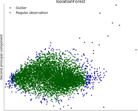
3.3 Sample Data pre-processing 3.3.1 Outlier removal - Isolation Forest

As the ground truth data were collected by different people and also consists of multiple sources (Field work, Inventory data), various errors (mislabeling) could be present. In order to reduce the chance of polluted training data, and thereby the possibility of biased parameters (Ben-Gal 2005), a way of outlier detection seemed necessary. An outlier itself is defined as:

(37)

Figure 18: PCA reduced visualization of outliers detected using Isolation Forest

An outlying observation, or “outlier,” is one that appears to devi-ate markedly from other members of the sample in which it occurs. (Grubbs 1969)

In this context it means a pixel of eg. Picea abies is either mislabeled as another species, or not representing forest at all. As hyperspectral data are high dimensional data, and also highly correlated consisting of redundant features, outlier detection methods using density or distance are not a good fit (Aggarwal et al. 2001). As this problem increases with availability of high dimensional data (Curse of dimensionality (Zimek et al. 2012)), other methods than using distance were proposed by (Kriegel et al. 2009, F. T. Liu et al. 2008).

For example the Isolation Forest is a method which is able to work with data where the existence of outliers is not known (F. T. Liu et al. 2012). It works by utilizing the abilities of a random tree to classify data, as outliers (or anomalies) are supposed to be "few and different" from the other sample data. This leads to the fact that outliers are classified closer to the root of the tree. The algorithm measures the path length, averaged over a forest of random trees for every sample. The path length is then treated as a measure of abnormality, detecting outliers. For this study the ground truth data (spectral values of the pixels) was checked for outliers using the IsoForest module7 provided in scikit-learn. In order to

(38)

visualize the result of the outlier detection using the Isolation Forest algorithm the dimensionality of the dataset was reduced using a Principal Component Analysis (PCA) and is shown in Figure 18.

4 Supervised Machine Learning

Supervised learning refers to a process that learns a function from a tulpe

(x1, y1),(x2, y2), ...,(xn, yn), of inputs (also called predictors) and outputs (also

called label), in order to predict the label of inputs where the output is not known. Every single input variable (instance, egx1) consists of multiple attributes (also

calledfeatures). Two typical examples of supervised learning are classification and regression tasks (Sammut et al. 2011). Given a data-setX, for some instances of the data-set (xi), a corresponding label is known (yi). This data is used in

order to train an algorithm to predict the corresponding label of the instances of X, where (yi) is unknown. So the algorithm defines a function (f), which

predictsyˆas denoted inyˆi=f(xi). Supervised classification is one of the most

frequently used procedures for classifying remotely sensed data (Richards 2012b). There are many algorithms available, designed for this task, such as Support Vector Machines (SVM), Neural networks, Nearest neighbor methods, Forests of randomized trees. However, because some of these algorithms were primarily designed to handle low-dimensional data, problems can arise when dealing with high dimensional data (Fuan et al. 2002).

4.1 Random Forest

One of the most prominent supervised classifiers at this time is the Random Forest algorithm proposed by Breiman (2001). It is a widely used implementation of random decision forests, and is based on an ensemble of decision trees (see Fig. 19).It is therefore categorized as an ensemble classifier. The Random Forest algorithm combines decision trees and bagging. Bagging (Bootstrap aggregating) is used in order to reduce the variance (Breiman 1996a), as a side effect it enables the estimation of the generalization error (OOB error). The samples are drawn at random with replacement from the training instances, the unused part of the samples is utilized to calculate the out-of-bag error (see 2.3.1). Each tree is grown with a randomly sampled feature set (random subspace method (Ho 1998)) selected for each split (4.8.2). This way the correlation between the single trees is decreased, which improves the accuracy of the algorithm (Hastie et al. 2009). IsolationForest.html

(39)

This method has shown to perform better than using bagging only, especially when many redundant features are present (Archer et al. 2008). In the original implementation of Random Forest, all trees take a vote on the predicted class (majority voting). The implementation applied in this study (Pedregosa et al. 2011) uses an averaged probability prediction (as seen in Fig. 40). However the differences should be negligible (Breiman 1996a).

Figure 19: Single tree showing first two levels of tree species classification using vegetation indices

The main advantages of random forests are: • Non parametric

• Robust against outliers • Embarrassingly parallel

• Achieves a high prediction accuracy with only tuning a few parameters (4.8) (Hastie et al. 2009, Cutler et al. 2012, Qi 2012)

Random forests are widely used in the field of environmental remote sensing for surface classification (Pal 2005, Gislason et al. 2006), in particular in combination with hyperspectral data (Crawford et al. 2003, Ham et al. 2005, Chan et al. 2008). It is also known as robust supervised learning method in general (Caruana et al. 2006, Fernández-Delgado et al. 2014).

4.2 Extremely randomized trees

Extremely randomized trees (ET) were developed by Geurts et al. (2006). The forest of randomized trees is based on RF, but the algorithm takes the random-ization to the next level. The trees are also grown using bagging for the samples

(40)

and the random subspace method, as described in section 4.1. But in addition cut points are set at random (chosen randomly among the training data) and the split point with the best result is selected in order to compute the split for all features present in the random subspace of the maximal features considered (4.8.2). In the default settings each tree is built from the complete training set (no bootstrapping) as a measure to further reduce bias, but it should be noted that in order to obtain the OOB score, bootsstrapping was used in this study.

4.3 Choosing one classifier

The decision which classifier to use was made based on several reasons. While both classifiers, Random Forest (RF) and Extremely randomized trees (ET), showed high stability after enough trees, Random Forest (RF) showed a minimally better performance regarding the error metrics (Fig. 24). On the other hand during evaluation of the classifiers and test runs, Extremely randomized trees (ET) classifier showed a better avoidance of over-fitting, especially when the DTM was used. But one of the biggest advantages regarding ET is the computational benefit (Geurts et al. 2006).

Intel(R) Core(TM) i7-6700K CPU @ 4.00GHz Fitting: 5 Fold cross validation:

RF: 3min 37s 10min 30s

ET: 0min 22.7s 1min 28s

Especially during the tuning of the classifier parameters (section 4.8) and cross-validation, this performance difference becomes apparent. As ET performs around

∼_{8 times faster, with the benefit of better avoidance of over-fitting (Geurts et al.}

2006), this algorithm was finally applied in this study.

4.4 Features

The previously describe available data sets (2.2.2 - 2.2.5), are combined for further processing to one single database (Table 7). Each individual measured or calculated property of an instance is calledfeature, eg. each band (λ) represents one feature. In total 275 features (||X||) are available.

(41)

Table 7: Available data for Machine Learning

Spectral Data LiDAR data

VNIR SWIR Vegetation indices DTM Treecount

131 Bands 133 Bands 9 Indices Meters above MSL Tree density

From all available data various combinations of features can be employed as input for classification and compared later on for their classification performance. All optional combinations used in this analysis are listed in Table 8 with an abbreviation.

Table 8: Combinations of features used

Spectral Data LiDAR data

Abbrv. VNIR SWIR VIs DTM Treecount

All X X X X X SpecInd X X X Spectral X X SWIR X SWIRFull X X X X VNIR X VNIRFull X X X X

For visualizing the effect of the DTM on the map accuracy (possible over-fitting), all feature combinations were also calculated with and without the DTM input. Also an additional run was conducted with a reduced number of bands (band selection (BS), see section 4.6). It should be mentioned that all vegetation indices (VIs) were calculated using both VNIR and SWIR bands (see 2.2.3). Thus the VIs are not supposed to replace the spectral bands, but to detect possible advantages by using them.

4.5 Feature engineering

In Machine Learning it is common to extend the feature space through applied domain knowledge. This happens by aggregating, combining or splitting features to create new features. This process is also called feature construction.

(42)

Feature construction [...] is a process that discovers missing relations among features and augments the space of features by inferring or creating additional compound features, and thus could expand the feature space.

H. Liu et al. (1998) As an example, if the relationship of the label of the two instances (x1 andx2)

depends mainly on the angle of two features, it can increase the classification result, if that relationship is added to the feature space. This approach of including the relationship of features in an analysis is not new in the field of applied remote sensing. Vegetation indices (2.2.3) have been in use since the 1970s (Bannari et al. 1995), and can be considered a feature construction method in the machine learning sense, as the aim is to construct new representations of the data by combining multiple bands.

4.6 Feature selection

In hyperspectral data exploitation it is common to apply band selection to the data in order to remove highly correlated bands and noise. Due to the large number of spectral bands the difference in information contained in bands close to each other is often minimal (Spectral redundancy, see Foody et al. 2004 and Richards 2012a). In Machine learning such an approach can be considered as Feature selection, as the goal is to reduce the numbers of features necessary for achieving a good classification. The main outcome of a reduction in features is the reduced computation time, while also the risk of over-fitting can be reduced (Bolón-Canedo et al. 2015), and the accuracy can be increased (Janecek et al. 2008). In addition Hänsch et al. (2016) have shown that due to the redundancy of information in correlated spectral bands, random forests are able to achieve an already very good classification result with less bands (see Figure 20). However Forests of randomized trees automatically determine which features are the most useful for class separation during the training phase (see 4.6.1). The amount of features used to construct a forest is one of the parameters tuned while optimizing the classifier (4.8.2). This study should not only output results of a classifier, but also aims at investigating how the prediction results are influenced by different approaches. Therefore, the decision was made to include some kind of band selection and perform the classification with and without it, in order to evaluate the influence of the removal of certain spectral bands on the classification result.

(43)

4.6.1 Feature importance

The Gini importance (mean decrease in impurity) measure can be used to rank the features according to their importance in the models ability for class separation. Alternatively, the mean decrease in accuracy could be used as well, however it has been proposed to use the Gini importance for studies with smaller sample sizes (Archer et al. 2008). The Gini importance is based on the Gini impurity and measures how often a feature was selected for a split. As splits based on Gini impurity try to produce pure nodes (Breiman 1996c), the features selected for a higher amount of splits resulting in purer splits, is considered more important than the other features. Or in other words the Gini importance is based on the weighted impurity decrease at all nodes the variable was used, averaged over all trees (Louppe et al. 2013). But studies have shown that using the Gini criterion for feature importance can be biased (Strobl, Boulesteix, Zeileis, et al. 2007). However this is only true if features are not of the same measurement scale. If only continuous features are used (eg. spectral data), feature importance based on the Gini criterion can be used for feature selection. But that still leaves a problem, because even so the algorithm scores features without bias, one still doesn’t know how many features are relevant. Especially as the Gini importance tends to rank the first features very high while for remaining features a sharp drop in importance is observed. Another problem is that the algorithm can’t differentiate between correlated features (Archer et al. 2008, Menze et al. 2009), and has problems scoring them correctly (Strobl, Boulesteix, Kneib, et al. 2008, Tolosi et al. 2011, K. Nicodemus 2011). The usage of feature importance is a highly controversial topic (Gregorutti et al. 2016) when correlated predictors are included. This does not change the prediction results, but from an analysis point of view the feature importance can’t be reliably used to distinguish important features from non important ones if the features are highly correlated. This makes feature importance unsuitable for feature selection when working with hyperspectral data.

4.6.2 Recursive feature elimination

Recursive feature elimination is a method where an estimator is trained repeatedly with a given set of features, and during every run one feature is left out. In a cross-validation loop the accuracy (the ratio of correctly predicted observations to the total amount of observations) of the classifier is evaluated to find the optimal number of features. That increases the stability of the selection results

(44)

by reducing the effect of the correlation on the importance measure (Gregorutti et al. 2016).

Figure 20: Recursive feature elimination for hyperspectral data. Showing an optimal number of 93 Bands

The recursive feature elimination clearly shows that the error rate for predictions with spectral data stabilizes after around 50 features (Figure 20). The algorithm itself determines 93 features as an optimal cut off point. But on the other hand the plot also shows that the error rate does not increase even if all features are used. The applied recursive feature elimination resulted in the selected bands shown in Figure 21 in red. For an overview, see Table 20

Figure 21: Selected bands in red on a sample vegetation spectrum (in blue, interpolated bands not shown).