FRACTAL DIMENSION FOR CLUSTERING AND
UNSUPERVISED AND SUPERVISED FEATURE
SELECTION
A thesis submitted to Cardiff University in candidature for the degree of
Doctor of Philosophy
by
Moises Noe Sanchez Garcia
Manufacturing Engineering Centre School o f Engineering
Cardiff University United Kingdom
UMI Number: U585577
All rights reserved
INFORMATION TO ALL USERS
The quality of this reproduction is dependent upon the quality of the copy submitted. In the unlikely event that the author did not send a complete manuscript and there are missing pages, these will be noted. Also, if material had to be removed,
a note will indicate the deletion.
Dissertation Publishing
UMI U585577
Published by ProQuest LLC 2013. Copyright in the Dissertation held by the Author. Microform Edition © ProQuest LLC.
All rights reserved. This work is protected against unauthorized copying under Title 17, United States Code.
ProQuest LLC
789 East Eisenhower Parkway P.O. Box 1346
ABSTRACT
Data mining refers to the automation of data analysis to extract patterns from large amounts of data. A major breakthrough in modelling natural patterns is the recognition that nature is fractal, not Euclidean. Fractals are capable of modelling self-similarity, infinite details, infinite length and the absence of smoothness.
This research was aimed at simplifying the discovery and detection of groups in data using fractal dimension. These data mining tasks were addressed efficiently. The first task defines groups o f instances (clustering), the second selects useful features from non-defined (unsupervised) groups of instances and the third selects useful features from pre-defined (supervised) groups of instances. Improvements are shown on two data mining classification models: hierarchical clustering and Artificial Neural Networks (ANN).
For clustering tasks, a new two-phase clustering algorithm based on the Fractal Dimension (FD), compactness and closeness of clusters is presented. The proposed method, uses self-similarity properties of the data, first divides the data into sufficiently large sub-clusters with high compactness. In the second stage, the algorithm merges the sub-clusters that are close to each other and have similar complexity. The final clusters are obtained through a very natural and fully deterministic way.
The selection o f different feature subspaces leads to different cluster interpretations. An unsupervised embedded feature selection algorithm, able to detect relevant and redundant features, is presented. This algorithm is based on the concept o f fractal dimension. The level o f relevance in the features is quantified using a new proposed entropy measure, which is less complex than the current state-of-the-art technology. The proposed algorithm is able to maintain and in some cases improve the quality of the clusters in reduced feature spaces.
For supervised feature selection, for classification purposes, a new algorithm is proposed that maximises the relevance and minimises the redundancy o f the features simultaneously. This algorithm makes use of the FD and the Mutual Information (MI) techniques, and combines them to create a new measure of feature usefulness and to
produce a simpler and non-heuristic algorithm. The similar nature of the two
techniques, FD and MI, makes the proposed algorithm more suitable for a straightforward global analysis o f the data.
ACKNOWLEDGEMENTS
I would like to express my deepest and sincere gratitude to my supervisor, Prof. D. T. Pham, for giving me guidance and support during all the stages of my research.
Special thanks to Dr. Michael S. Packianather and Dr. Marco Castellani with whom I always was able to find fruitful discussions regarding my work.
I would like also to thank my family for their support and encouragement through all my life and my girlfriend Rach for all the love.
Thanks to the members o f the MEC machine learning group for sharing interesting ideas and useful comments in our weekly meetings.
Thanks to the colleagues in the lab I worked for helping to keep my spirit up.
I would like to thank CONACYT (COnsejo NAcional de Ciencia Y Tecnologia) Mexico for giving me the financial means o f pursuing a Ph.D education.
DECLARATION
DECLARATION
This work has not previously been accepted in substance for any degree and is not concurrently submitted in candidature for any degree.
S igned (Moises Noe Sanchez Garcia) Date 31/05/2011
STATEMENT 1
This thesis is being submitted in partial fulfillment of the requirements for the degree of Doctor of Philosophy (PhD).
Signed (Moises Noe Sanchez Garcia) Date 31/05/2011
STATEMENT 2
This thesis is the result of my own independent work/investigation, except where otherwise stated. Other sources are acknowledged by explicit references.
Signed (Moises Noe Sanchez Garcia) Date 31/05/2011
STATEMENT 3
I hereby give consent for my thesis, if accepted, to be available for photocopying and for inter-library loan, and for the title and summary to be made available to outside organisations.
J
TABLE OF CONTENTS
Page
Abstract
iAcknowledgements
ivDeclaration
vList of Figures
ixList of Tables
xiiAbbreviations
xiiiNomenclature
xvChapter 1 Introduction
1
1.1 Background
1
1.2 Fractal Mining
3
1.3 Statistical Entropy
3
1
.4
Mutual Information
4
1.5 Motivation
4
1.6 Aim and Objectives
5
1.7 Outline of the thesis
6
Chapter 2 Background
8
2.1 Fractal Dimension
8
2.1.1 Self-Similarity
8
2.1.2 Box Counting Dimension
10
2.2 Clustering
11
2.2.2 Number of clusters
14
2.2.3 Cluster Validity
25
2.3 Feature Selection Approaches
15
2.3.1 F ilter Approach
16
2.3.2 Wrapper Approach
17
2.3.3 Embedded approach
18
2.4 Unsupervised Feature Selection Approaches
20
2.5 Unsupervised Feature Relevance
21
2.6 Statistical Entropy
22
2.6.1 Entropy in Data Mining
23
2.6.2 Entropy as Relevance Measure
25
2.7 Search Techniques Overview
25
2.7.1 Sequential Selection Algorithms (SSA)
26
2.7.1 Second generation of SSA
27
2.8 Relevance in Features
31
2.8.1 Relevance Approaches in FS
23
2.8.2 Relevance versus Optimality
25
2.9 Feature Redundancy
37
2.10 Mutual Information
39
2.11 Redundancy Feature Analysis
37
2.10 Redundancy Feature Analysis
39
2.11 Summary
40
Chapter 3 Divisive Fractal Clustering Approach
41
3.1 Preliminaries
41
3.2 Hierarchical Clustering
42
3.2.1 Agglomerative analysis
45
3.3 Fractal Clustering
39
3.4 Proposed Algorithm
48
3.4.1 Second Phase
50
3.4.2 Stopping Criterion
50
3.4.3 Number of clusters
50
3.4.4 Refining Step
52
3.4.5 Evaluation Measure
52
3.4.5 DIANA (Divisive Analysis)
46
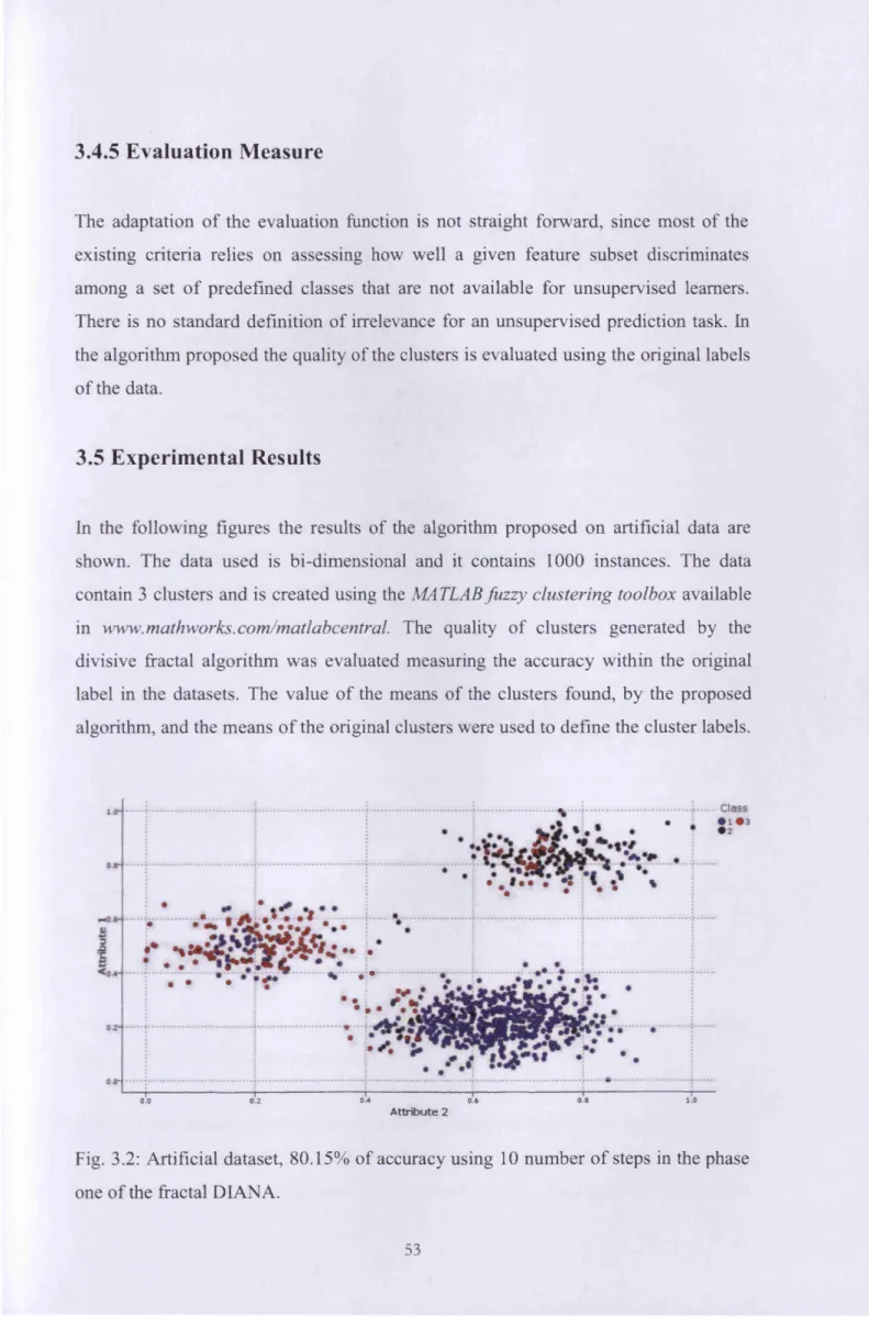
3.5 Experimental Results
52
3.3 Summary
55
Chapter 4 Unsupervised Feature Selections
56
4.1 Preliminaries
56
4.2 Unsupervised Feature Selections
57
4.3 Unsupervised Relevance and Redundancy in Features 59
4.4 Fractal Dimensionality Reduction
60
4.5 Statistical Entropy Relevance Estimation
63
4.6 Proposed Algorithm
65
4.6.1 Unsupervised Redundancy
66
4.8 Experimental Result
68
4.7 Discussion
94
4.9 Summary
95
Chapter 5 Supervised Feature Selection
94
5.1 Preliminaries
94
5.2 The Filter Approach
96
5.2.2 Maximal Relevance Minimum Redundancy (mRMR)139
5.2.3 Supervised Redundancy
100
5.3 Algorithm Proposed
100
5.3.1 Algorithm Implementation
102
5.4 Experimental Result
103
5.5 Discussion
138
5.6 Summary
138
Chapter 6 Conclusion
191
6.1 Contribution
137
6.2 Conclusion
138
6.3 Suggestions for Future Research
139
Appendix A
Back-Propagation Algorithm
140
Appendix B
Supervised feature Selection Algorithms
144
Appendix C
PC A projections o f the benchmark datasets used
146
Appendix D
A two step Clustering Algorithm
140
LIST OF FIGURES
Figure
Page
2.1 Self-similarity in 1, 2 and 3 dimension. New pieces when each line segment
is divided by M. 8
2.2 a) Sierpinsky pyramid, b) Sierpinsky triangle. 9
2.3 Illustration o f box-counting method, in every step the size of the grid r is
decreased in h alf to analyse the data in different level of resolutions. 1 0
2.4 Points generated to calculate the FD o f an object. 11
2.5 Filter Approach 17
2.6 Wrapper Approach 18
2.7 Embedded approach 19
3.1 Diagram for relevant Features 33
3.2 DIANA 49
3.3 Artificial dataset, 80.15% o f accuracy using 10 number o f steps in the phase
one o f the fractal DIANA. 53
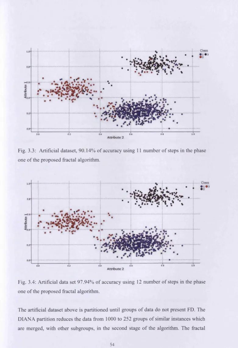
3.4 Artificial dataset, 90.14% o f accuracy using 11 number o f steps in the phase
one o f the proposed fractal algorithm. 53
3.5 Artificial dataset 97.94% o f accuracy using 14 number of steps in the phase
one o f the proposed fractal algorithm. 54
3.6 a) Sierpinsky pyramid and, b) Sierpinsky triangle 61
3.7 Illustration of the calculation o f the FI 65
3.8 Breast cancer Wisconsing unsupervised and supervised FS comparison 70
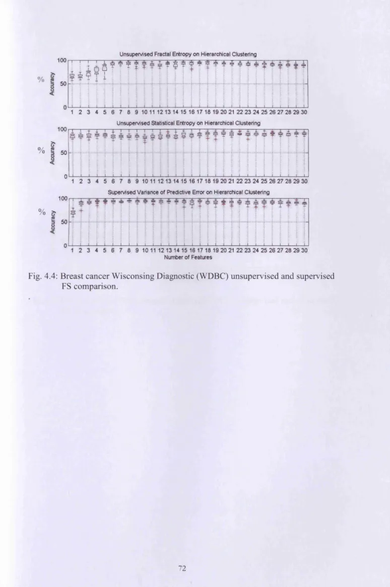
3.9 Breast cancer Wisconsing diagnostic (WDBC) unsupervised and supervised
FS comparison. 71
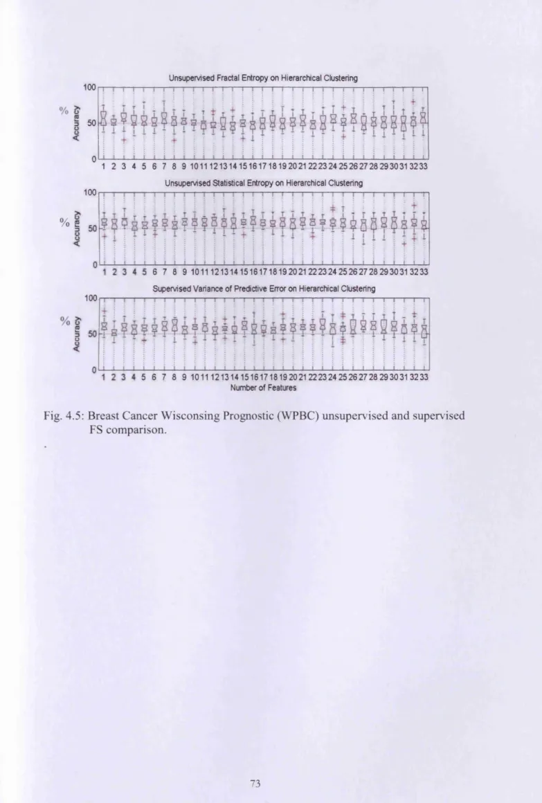
3.11 Breast Cancer Wisconsing prognostic (WPBC) unsupervised and supervised
FS comparison. 72
3.12 Australian credit approval unsupervised and supervised
FS comparison 73
3.13 Echocardiogram unsupervised and supervised FS comparison 74
3.15 Statlog Heart unsupervised and supervised FS comparison 76
3.16 Hepatitis unsupervised and supervised FS comparison 77
3.17 Ionosphere unsupervised and supervised FS comparison 78
4.1 Iris unsupervised and supervised FS comparison 79
4.2 Lymphography unsupervised and supervised FS comparison 80
4.3 Parkinson (K-means) unsupervised and supervised FS comparison 81
4.4 Pima indian diabetes unsupervised and supervised FS comparison 82
4.5 Lenses unsupervised and supervised FS comparison 83
4.6 Glass identification unsupervised and supervised FS comparison 84
4.7 Tae unsupervised and supervised FS comparison 85
4.8 Mammography classes unsupervised and supervised FS comparison 8 6
4.9 SPECTF Heart unsupervised and supervised FS comparison 87
4.10 Vehicle unsupervised and supervised FS comparison 8 8
4.11 Vowe context unsupervised and supervised FS comparison 89
5.1 Wine unsupervised and supervised FS comparison 90
5.2 Zoo unsupervised and supervised FS comparison 91
5.3 Wood (real application) unsupervised and supervised FS comparison 92
5.4 Traditional framework o f feature selection 101
5.5 Proposed framework o f feature selection 101
5.6 Australian Credit approval SFS comparison 107
5.7 Echocardiogram SFS comparison 108
5.8 Ecoli SFS comparison 109
5.9 Heart SFS comparison 110
5.10 Hepatitis SFS comparison 111
5.11 Image Satellite (Statlog version) SFS comparison 112
5.12 Image Segmentation SFS comparison 113
5.13 Letter recognition SFS comparison 114
5.14 Ionosphere SFS comparison 115
5.15 Lenses SFS comparison 116
5.16 Mammography Masses SFS comparison 117
5.17 Parkinson SFS comparison 118
6.1 Shuttle SFS comparison 119
6.2 Sonar SFS comparison 120
6.4 Vehicle SFS comparison 122
6.5 Breast Cancer (wdbc) SFS comparison 123
6 . 6 Wine SFS comparison 124
6.7 Pima Indian diabetes SFS comparison 125
6 . 8 Glass SFS comparison 126
6.9 Lymphography SFS comparison 127
6.10 SPECTF heart SFS comparison 128
6.11 Tae SFS comparison 129
6.12 Zoo SFS comparison 130
6.13 Breast Cancer W isconsing Prognostic (WPBC) SFS comparison 131
6.14 Iris SFS comparison 132
6.15 Breast Cancer SFS comparison 133
6.13 Vowe Context SFS comparison 134
LIST OF TABLES
Table
Page
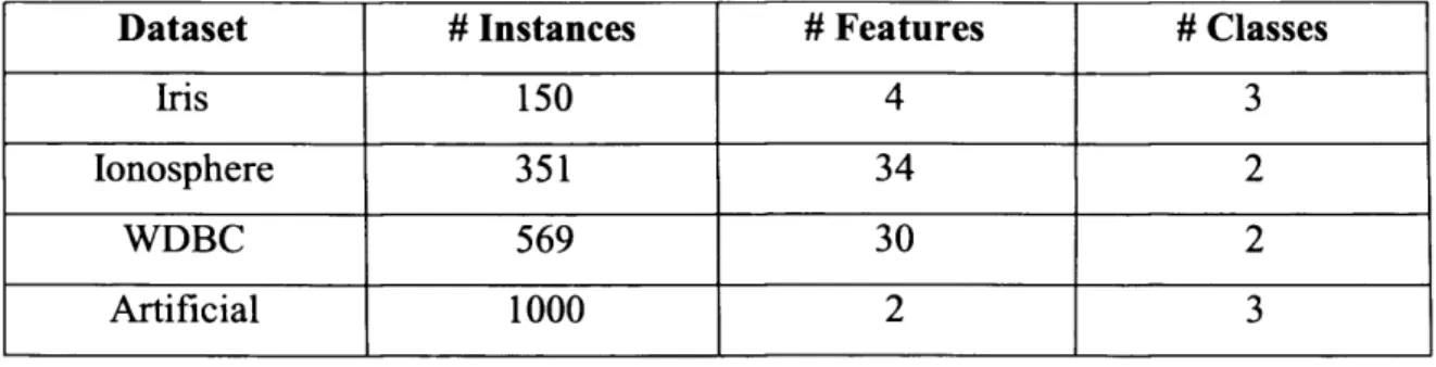
3.1 Benchmark datasets and artificial dataset used to test and compare
the Fractal clustering algorithm, proposed and original version. 54
3.2 Experimental results using benchmark and artificial datasets. 95
3.3 Experimental results using the benchmark and artificial datasets 55
used Table 3.2 for the FC algorithm proposed by Barbara (2003).
4.1 Description o f benchmark datasets. 69
ABBREVIATIONS
FD Fractal Dimension
CAD Computer Aided Design
CAM Computer Aided Manufacturing
DNA deoxyribonucleic acid
MI Mutual Information
FS Feature Selection
Jstor Journal o f the Royal Society
AI Artificial Intelligence
SOM Self-Organizing Map
DP Dirichlet process
BIC Bayes Information Criterion
AIC Akiake Information Criterion
MML Minimum Message Length
GMM Gaussian Mixture Model
UFS Unsupervised Feature Selection
EM Expectation M aximisation
RIS Ranking Interesting Subspaces
ID3 Iterative Dichotomiser 3
SBS Sequential backward selection
SFS Sequential forward selection
GSFS Generalised Sequential Forward Selection
GSBS Sequential backward Selection
PTA Plus 1-Take Away
GPTA General Plus 1-Take Away
GPTA General Plus 1-Take Away
SBFS Sequential Backward Floating Selection
SFFS Sequential Forward Floating Selection
AFS Adaptive Floating Search
OS Oscillating search
SA Simulated Annealing
PCA Principal Component Analysis
FC Fractal Clustering
DIANA Divisive Analysis
FI Fractal Impact
UFS Unsupervised Feature Selection
FDR Fractal Dimension Reduction
PFD Partial Fractal Dimension
FS Feature Selection
mRMR maximum Relevance and Minimum Redundancy
UCI University o f California in Irvine
ANN Artificial Neural Network
NOMENCLATURE
N Number o f features D Data Space X Y Random variables A Data set B Number o f boxesr Length o f the box side
i Fractal Dimension
V Number o f object in a reduced version o f the full set
TJ(S) Number o f boxes occupied with
K Number o f clusters
s
Microstates in a non-uniform distributionm Thermodynamic state
N*
Number o f boxes needed to cover an objectI Number of instances
S(r) Sum o f points in each cell at each resolution r
x i Data point
M Number o f dimension
E Entropy
S Similarity measure
D* Distance between instances
a Constant o f similarity measure
k* k th dimension
e f Entropy function proposed
Fractal ratio to measure redundancy in the ith feature
ApD Difference between partial and total fractal dimension
T Original variable set o f features
/ ith feature in the data
P(C) Probability o f different classes
H(C / F ) Conditional Entropy given the
c classes
I(A;B) Mutual information between two variables
Chapter 1
Introduction
This chapter presents a general background o f methods, motivation and objectives adopted in this research. At the end, the structure of the thesis is outlined.
1.1 Background
Euclidean geometry has endured over the centuries because it provides a good basis for modelling the world, but there are many circumstances where it fails. An example of this is when in 1950 the English mathematician, Lewis Fry Richardson, needed to estimate the coast line o f Great Britain. Richardson soon realized that the length of the coastline was indeterminate because it depended on the resolution with which the measurements were made. In order to describe non-Euclidean structures, in 1977 the mathematician Benoit Mandelbrot developed the concept of a dimension that had no integer values and was capable o f performing multi-resolution analysis. The term given by Mandelbrot to the dimension was Fractal. Since 1977 FD has attracted attention as a practical tool in many branches of science where Euclidean distance is used. Scientific fields such as hydrology, geophysics, biology and communication systems are just some examples (Mandelbrot and Ness, 1968).
When researchers realized how well fractals mimicked nature, they started to explore how to measure and apply the FD in their investigations. The FD has been used as a method o f quantifying the complexity o f a wide variety of materials, objects and phenomena. For example the growth o f tree structures; nerve cell growth and degeneration, osteoporosity, metal fatigue, fractures, diffusion and electrical discharge phenomena. The FD can measure the texture of a surface and is able to replace or augment Fourier methods by providing an index of surface roughness quantification (Borodich, 1997).
Image compression is another field in which fractals have been introduced and proven useful. Fractal image compression methods were developed by Michael Barnsley in
1987 when he set up his company, Iterated Systems. Most images exhibit a high degree o f redundancy in their information content: for example most adjacent pixels will be the same or of similar colour or intensity. This redundancy can be used to repack the image so that it takes up less storage space (Barnsley, 1988).
Contemporary Computer Aided Design (CAD/computer aided manufacturing (CAM) theories and systems are well developed only for Euclidean analytical objects, lines, curves and volumes. However, there are still many types of objects such as flexible objects with a deformable geometry, and non-Euclidean geometrical objects, that cannot be modelled by the current CAD representation schemes. In this case, the FD can be used to mathematically define these types of products (Chiu et al., 2006).
1.2 Fractal Mining
The goal of data mining is to find patterns. Classical modelling approaches look for Gaussian patterns that often appear in practice. However, distributions such as Poisson and Gaussian, together with other concepts like uniformity and independence, often fail to model real distributions. Work done in data mining and pattern recognition shows how fractals can often reduce the gap between modelling and reality. FD is used in the following ways:
• To find patterns in a cloud o f points embedded in the hyper space.
• To find patterns in time sequences useful in characterization and prediction.
• Graph representation e.g. social or computer networks.
The first is when multidimensional clouds of points appear in traditional relational databases, where records with N attributes become points in N-D spaces (age, blood pressure, etc), for example medical databases, 3-D brain scans (Arya et al., 1993) and multimedia (Faloutsos et al., 1994) databases. In these settings the distribution o f the N-d points is seldom uniform. It is important to characterize a deviation to this uniformity in a concise way (Agrawal and Srikant, 1994) and to find accurate and short descriptions in the databases. The characterization o f the data helps to reject some useless information and to provide hints about hidden rules.
The second task is when data changes through time. Time sequences appear very often in many o f data applications. For example, there is a huge amount of literature in linear (Box et al., 1994) and non-linear forecasting (Castagli and Eubank, 1992) as well as in sensor data (Papadimitriou et al., 2003).
The third task is so general that it seems to be apparent everywhere, precisely because graph representation has a large number of applications, for instance in the world wide web which is probably the most impressive real network. So finding patterns, laws and, regularities in large real networks has numerous applications. Examples include: Link analysis, for criminology and law enforcement (Chen et al., 2003); analysis of virus propagation patterns on social/e-mail networks (Wang et al., 2000). Another application is the analysis o f empirical data collections of DNA segments, called Networks o f Regulatory Genes to indicate possible gene connections and interactions they have with proteins to perform their functions (Barbasi, 2002).
An extended enterprise is a type o f network comprising interconnected organizations sharing knowledge and manufacturing resources. The individual organizations team up with one another so that their competitive advantage can be improved. Fractals are introduced into the construction o f extended enterprises to enable simpler performance and transparency in terms o f modality, information, functionality and time (Hongzhao et al., 2004).
1.3 Statistical Entropy
Entropy is considered a form o f information and can be used to measure uncertainty of random variables (Fast, 1962). Unlike energy, information is not conserved. However, an analogy between information and energy is interesting because they share several properties. Energy and information can exist in any region o f space, can flow from one place to another, can be stored for later use, and can be converted from one form to another.
In the context o f physical systems uncertainty is known as entropy. In communication systems the uncertainty regarding which actual message is to be transmitted is also
known as the entropy of the source. The general idea is to express entropy in terms of probabilities, with the quantity dependent on the observer (features in the case of data). One person may have different knowledge of the system from another one, and therefore would calculate a different numerical value for entropy.
Statistical entropy is a technique that can be used to estimate probabilities more generally. The result is a probability distribution that is consistent with known constraints expressed in terms of averages. This principle has applications in many domains, but was originally motivated by statistical physics, which attempts to relate macroscopic, measurable properties o f physical systems. Physical systems, from the point of view o f information theory, provide a measure of ignorance (or uncertainty, or entropy) that can be mathematically calculated.
1.4 MI (Mutual Information)
MI is a measure that shows the amount of information between two random variables x and y. In MI conditional entropy is used to calculate the reduction of uncertainty
about the variable x, when y is known (Cover and Thomas, 2006). For example MI is
used in text classification to calculate the amount of information between certain words and the rest o f the document (Michel et al., 2008). MI is used in speech recognition and to find combinations o f audio feature stream (Ellis and Bilmes, 2000). Other areas o f application o f MI are probabilistic decision support, pattern recognition, communications engineering and financial forecast (Fayyad et al., 1996). More recently, MI has been widely used in data mining due to its robustness to noise and to data transformations.
1.5 Motivation
Finding groups in data is a practical way to handle large amounts o f data. Powerful mathematical and statistical concepts such as fractals, MI and entropy are tools that work well independently, which have never been combined before, for data mining.
A combination o f these tools to simplify supervised and unsupervised data mining methods is addressed in this research as set out below:
• Divisive hierarchical clustering algorithms are not generally available in the literature and have rarely been applied due to their computational intractability. In this research a combination of hierarchical clustering and fractals is proposed to make divisive clustering more accessible than existing methods such as that developed by Kaufman and Rousseeuw (2005).
• To identify important features, when labels are not available, in a dataset is a problem without a direct solution. An unsupervised feature selection approach based on fractals instead o f Euclidean geometry is developed to improve on a solution proposed in (Dash et al., 1997).
• Common supervised feature selection algorithms (Liu et al., 2008, Peng et al., 2005) rely mainly on heuristics tools such as search techniques and learning machines to find correlations at the cost o f burdening the feature selection process. FD in combination with other tools can alleviate computational burden in a pure mathematical basis.
1.6 Aim and Objectives
The overall aim objective o f the research is to combine fractals, statistical entropy and MI techniques for the development o f new algorithms, to simplify the detection of groups in data under an unsupervised and a supervised framework.
The specific objectives are summarised as follows:
• To develop a new simpler top-down hierarchical clustering algorithm that uses the FD as a similarity measure. The methodology gives the algorithm the capability to find clusters without any initialization step which is needed in previous fractal clustering algorithms.
• To develop an unsupervised Feature Selection (FS) algorithm that combines the FD and statistical entropy to detect useful features. The use of the FD reduces the complexity of the statistical entropy calculation and the removal of irrelevant features.
• To develop a supervised FS algorithm that combines FD and MI to maximize
the relevance and minimize the redundancy o f features simultaneously. The algorithm should select useful features without using any intermediate or heuristic subset evaluation step as is used in current FS frameworks.
1.7 Outline of the thesis
Chapter 2: This chapter gives an overview of classical FS approaches and clustering. Fractals, entropy and MI concepts followed by their applications in data mining are introduced.
Chapter 3: This chapter proposes a new clustering approach to find natural clusters in data. The algorithm uses the FD as a similarity measure among instances. The divisive approach used in the algorithm simplifies the analysis procedure of previous Fractal Clustering (FC) algorithms.
Chapter 4: In this chapter, a new Unsupervised Feature Selection (UFS) algorithm that ranks the features in terms o f importance is proposed. The algorithm takes advantage of mathematical properties o f the FD to reduce the complexity of the entropy function, to calculate relevant features under an unsupervised framework.
Chapter 5: In this chapter a new FS method that uses MI and FD is presented. The proposed method maximises the relevance and minimises the redundancy of the attributes simultaneously. The new method proposes a simpler framework for the evaluation of useful features.
Chapter 6: In this chapter, the conclusions and the main contributions of this thesis are presented. Suggestions for future research in this field are also provided.
Chapter 2
Background
This chapter presents an overall description of the basic concepts, FD, statistical entropy and MI that are used in this research. The chapter also introduces clustering and unsupervised and supervised feature selection approaches and gives recent examples of clustering and feature selection techniques.
2.1 Fractal Dimension
Most of the objects that are present in nature are very complex and erratic in having a Euclidean geometric structure. Mandelbrot proposed the concept of fractal in trying to address a model able to describe such erratic and imperfect structures. Since Mandelbrot, (1977) proposed the technique of FD to quantify structures, it has attracted the attention o f mathematicians (Flook, 1996), computer engineers and scientists in various disciplines. Mathematicians introduced FD to characterize self similarity to overcome the limitations o f traditional geometry (Mandelbrot, 1982) (Schroeder, 1991). Engineers and scientists in the area of pattern recognition and image processing, have used the FD for image compression (Barnsley, 1988), image medical processing (Zhuang and Meng, 2004), texture segmentation (Chaudhuri and Sarkar, 1998), face recognition (Zhao et al., 2008), de-noising (Malviya, 2008), and feature extraction (Traina et al., 2000). Physicists, chemists, biologists and geologists have used the FD in their respective areas as well. Fractal theory is based on various dimension theories and geometrical concepts. There are many definitions of fractals (Mandelbrot, 1982). In this thesis, a fractal is defined as a mathematical set with a high degree of geometrical complexity. This complexity is useful to model numeric sets such as data and images.
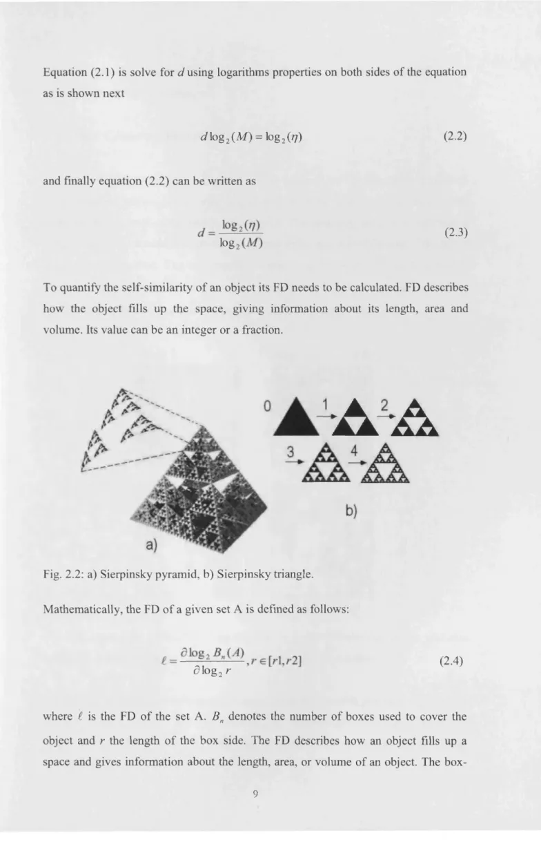
2.1.1 Self-Similarity
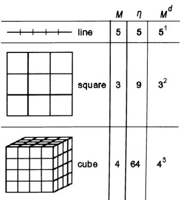
One of the characteristics of fractals is self-similarity as shown in Figure 2.1 by Sierpinsky pyramid and triangle. This property defines the geometrical or statistical likeness between the parts of an entity (dataset) and the whole entity (dataset).
Self-similarity implies a scaling relationship when little pieces of an object are exact smaller copies o f the whole object, i.e., smaller pieces of a fractal will be seen at finer resolution. Self-similarity specifies how the small pieces are related to the large pieces, thus self-similarity determines the scaling relationship. For example, consider a line segment to measure its self-similarity a line is divided into M smaller line segments, this will produce 77 smaller objects. If the object is self-similar each of the
77 smaller objects is an exact but reduced size copy of the whole object. The self
similarity d can be calculated direct from the equation
T] = M d (2.1)
m
n
M d
line
square
cube
Fig. 2.1: Self-similarity in 1, 2 and 3 dimension. 77 new pieces when each line
Equation (2.1) is solve for d using logarithms properties on both sides of the equation as is shown next
d log 2 (M ) = log 2 (77) (2.2)
and finally equation (2.2) can be written as
d = (2.3)
log 2(M )
To quantify the self-similarity of an object its FD needs to be calculated. FD describes how the object fills up the space, giving information about its length, area and volume. Its value can be an integer or a fraction.
■ArA
Fig. 2.2: a) Sierpinsky pyramid, b) Sierpinsky triangle.
Mathematically, the FD of a given set A is defined as follows:
dlo g 2 r (2.4)
where £ is the FD of the set A. Bn denotes the number of boxes used to cover the
object and r the length of the box side. The FD describes how an object fills up a space and gives information about the length, area, or volume of an object. The
box-counting method illustrated in Fig (2.3) is probably the most popular method due to its simplicity and good accuracy.
2.1.2 Box Counting Dimension
The box counting dimension is a useful way to measure the FD. The method consists in covering an object (data) with a grid and counting how many boxes the grid contains, for at least some part of the object. The counting process is repeated a certain number of times (resolutions), each time using boxes half the size of the boxes used the previous time. The box counting method calculates the FD dimension using the slope, shown in Fig (set number), of the plot log(rj(S)) versus log(l/ S) where
rj(S) is the number of boxes occupied and r is the size of the box.
Step 1
r
Step 2
r/2
Step 4
r/8
Fig. 2.3: Illustration of box-counting method, in every step the size of the grid r is decreased in half to analyse the data in different level of resolutions.
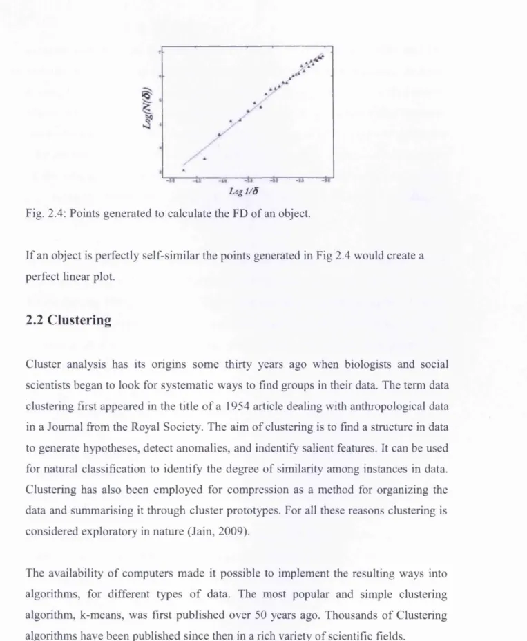
Each of the resolution in each step o f the box-counting method generates a point like the ones show in Fig 2.4. The quantity for the first resolution corresponds to the first point up-right of the graph, and the last resolution corresponds to the last point bottom-left.
Log 1 /5
Fig. 2.4: Points generated to calculate the FD of an object.
If an object is perfectly self-similar the points generated in Fig 2.4 would create a perfect linear plot.
2.2 Clustering
Cluster analysis has its origins some thirty years ago when biologists and social scientists began to look for systematic ways to find groups in their data. The term data clustering first appeared in the title of a 1954 article dealing with anthropological data in a Journal from the Royal Society. The aim of clustering is to find a structure in data to generate hypotheses, detect anomalies, and indentify salient features. It can be used for natural classification to identify the degree of similarity among instances in data. Clustering has also been employed for compression as a method for organizing the data and summarising it through cluster prototypes. For all these reasons clustering is considered exploratory in nature (Jain, 2009).
The availability of computers made it possible to implement the resulting ways into algorithms, for different types of data. The most popular and simple clustering algorithm, k-means, was first published over 50 years ago. Thousands of Clustering algorithms have been published since then in a rich variety of scientific fields.
Nowadays clustering is applied in different fields, such as: Geosciences, political science, marketing, Artificial Intelligence (AI), chemometrics, ecology, economics, medical research, psychometrics. Since the eighteenth century researches such as Linnaeus and Sauvages have provided extensive classification of animals, plants,
minerals and diseases. In astronomy Hertzprung and Russell classified stars into various categories using their light intensity and their surface temperature. In social science for example behaviour and preferences are usually used to classified people. Marketing tries to identify market segments which are structured according to similar needs of consumers (Arabie and Hubert, 1994). In geography the objective is to group different types o f regions. In medicine discriminating different types of cancer is one of the main applications as well as studying the genome data (Brandon et al., 2009). In chemistry classifying compounds and in history grouping archaeological discoveries, are other uses o f clustering.
Image segmentation, a branch o f AI, is an important problem in computer vision which is being formulated as a clustering problem (Jain and Dubes, 1988a, Frigui and Krishnapuram, 1999, Shi et ah, 2000). Automatic text recognition can be efficiently performed using hierarchical clustering techniques (Iwayama and Tokunaga, 1995). Clustering is also used in planning group services to deliver engagements for workforce management (Hu et ah, 2007).
2.2.1 Clustering Techniques
Clustering methods can be broadly classified into two categories: partitioning and hierarchical methods (finding groups in data). In partitioning methods the basic idea is to construct k clusters. In each cluster there is at least one object and each object must belong to exactly one o f the clusters. To satisfy this, there must be at least as many objects as there are clusters. In partitioning methods the number of clusters is given by the user. Not all values o f k lead to a “natural clustering”, so it is suggested to run the algorithm a few times using different values for k. A different option is to
leave the computer to decide the number k by trying many possible values and
choosing the one that is best at satisfying a particular condition.
Partitioning methods try to find a “good” set o f clusters in which the members in each are close or related to one another, and the members of different clusters are far apart or very different. The goal is to uncover a structure that is already present in the data.
cluster representatives (centroids) randomly, and assign each object to the cluster with its representative closest to the object. The procedure iterates until the distances squared between the objects and their representatives is minimized. Extension of k- means and k-medoids for large databases is CLARANS and BIRCH (Zhang et al., 1996). Other types o f partitioning methods are those which identify clusters by detecting areas o f high density object population. DBSCAN (Ester et al., 1996) finds these regions, which are separated by low density points, by clustering together instances in the same dense region. Self-Organizing Map (SOM) is an effective clustering algorithm (Kohonen, 1982) that can converge into optimal partitions according to similarities in the data. The SOM performs with prototype vectors that themselves can be associated to each cluster centroid. There are different versions of the SOM algorithm that try to overcome the measure of similarity among objects (Alahakoon and Halgamuge, 2000).
Hierarchical methods are among the first techniques developed to perform clustering. Unlike partitioning methods, hierarchical methods do not divide the data in a
determined number o f clusters. In theory they deal with all the values of k from one to
n which is the number o f elements in the data. When the partition has k= l clusters,
all the instances are together in the same cluster, and when the partition has k=n every
instance is considered a cluster. The only difference between k=r and k=r+l is that one o f the r clusters is divided to obtain r+1 clusters. Note that hierarchical algorithms can be used to generate a partition by specifying a threshold on the similarity o f the instances.
There are two types of hierarchical techniques. The first is called agglomerative, and the second, divisive. They construct their hierarchy in opposite directions, usually causing different results. The agglomerative approach builds clusters by merging two smaller clusters in a bottom-up mode. All the clusters together form a tree where leafs are the generated clusters and the root is the group with all the data instances. The divisive approach splits a cluster into two smaller ones in a top-down mode forming also a tree, the root in this case is the opposite to that in the agglomerative approach. However the tree structure is not exactly the same and depends crucially on the criteria used to choose the clusters to merge and split.
Hierarchical approaches have the disadvantage that they cannot correct what has been done in previous steps. In fact, once the agglomerative approach has joined two clusters, they cannot be separated any longer. In the same way when a divisive algorithm has divided an object, it cannot be reunited. However this limitation, in both hierarchical methods, is a key to achieve small computational times. On the other hand, hierarchical techniques do not really compete with partitioning approaches as they describe the data in a totally different way. The most well-known hierarchical algorithms are single-link and complete-link. Xiong et al., (2009) proposed a hierarchical divisive version o f k-means called bisecting k-means, that recursively partitions the data into two clusters at each step.
2.2.2 Number of clusters
To determine how many clusters are in a dataset has been one of the main problems in clustering. Very often, clustering algorithms are run with different values of number of clusters (AT); the best value for K is selected based on a predefined criterion. It is not easy to determine automatically the number o f clusters, the task casts into the problem o f model selection. The Dirichlet Process (DP) (Ferguson, 1973) (Rasmussen et al., 2009) proposes a probabilistic model to derive a posterior distribution for the number of clusters, from which the most likely number of clusters can be computed. Other techniques to calculate the number o f clusters are Bayes Information Criterion (BIC) and Akiake Information Criterion (AIC). (Tibshirani et al., 2001) use gap statistics assuming that when the data is divided into an optimal number of clusters, the partition is more resilient to random perturbations. Figueiredo et al., (2006), Jain and Flynn, (1996) use the MML (Minimum Message Length) criteria together with GMM (Gaussian Mixture Model). This approach starts with a large number of clusters which are gradually reduced if the MML criterion is minimized.
2.2.3 Cluster Validity
Cluster validity procedures intend to evaluate qualitatively and objectively the results of the cluster analysis. There are three basic criteria in which cluster validity can be performed: internal, relative, and external (Jain and Dubes, 1988). The internal
criterion compares the fit between the structure generated by the clustering algorithm and the data using the data alone. Hirota and Pedrycz (1985) propose a way of evaluating the fuzzy clustering methods using probabilistic sets and entropy characterisation. The relative criterion compares multiple structures that are generated by the same or by different algorithms, and decides which one of them is better. The external criterion measures the performance by matching the cluster structure to a priori information namely the class labels.
There is no best clustering algorithm. Each cluster algorithm imposes a structure on the data either implicitly or explicitly. When there is a good match between the model and the data, generally good partitions are obtained. Since the structure of the data is not known in advance, several approaches need to be tried before determining the best clustering algorithm for the application at hand. The idea of no clustering algorithm is the best is partially captured by “the impossibility theorem”. This theorem states that no single clustering algorithm simultaneously satisfies three basic axioms of clustering. The first is scale invariance, i.e. an arbitrary scaling of the similarity metric must not change the clustering results. The second axiom is richness, i.e. the clustering algorithm must be able to achieve all possible partitions of the data. The third is consistency, i.e. shrinking within cluster distances and stretching between- cluster distances, the clustering results must not change (Kleinberg, 2002).
The development o f a top-down hierarchical clustering algorithm is presented in chapter four. The algorithm uses FD as a similarity measure. The validation of the clusters is done using the class label (Dash et al., 1997).
2.3 Feature Selection Approaches
The objective of FS is to find a set o f features of a certain size that provide the largest generalization and stability in data predictions. This has been mainly performed by selecting relevant and informative features that increase the efficiency of existing learning algorithms. FS is one o f the central problems of machine learning so many algorithms incorporate the FS step in their framework. FS can have some other motivations such as:
• General data reduction - to limit storage requirements and increase algorithm speed.
• Feature set reduction - to save resources in the next round of data collection or
during its utilization.
• Performance improvement - to gain in predictive accuracy in the predictions.
• Data understanding - to gain knowledge about the process that is generated by the data or simply to visualize the data.
A critical aspect o f FS is to properly assess the quality of the features selected:
• Evaluation criterion definition (relevance index or predictive power).
• Evaluation criterion estimation (or assessment method).
Two of the main frameworks developed for feature selection are filters and wrappers. Both frameworks differ mainly in the way they evaluate the quality of the features. Filters uses evaluation criteria that does not employ feedback from learning machines for example criteria such as relevance index based on correlation coefficients or test statistics are examples o f these criteria. Wrappers on the other hand use the feedback of the learning machine to assess the quality of the features. There is a third approach for feature selection called the embedded method which incorporates the feature subset selection and evaluation in the learning machine (predictor) (Guyon et al., 2006).
2.3.1 Filter approach
The filter method, termed in (John et al., 1994), forms part of feature selection algorithms that are independent of any learning method. Such a method performs without any feedback from predictors and uses the data as the only source o f
performance evaluation. These characteristics make the filter method the least computationally expensive approach and the least prone to overfit the learning machine.
All features ►
Fig. 2.5: Filter Approach.
The filter approach has a framework in which FS is performed as a pre-processing step for learning. In this framework there is no connection between the learning machine and the FS algorithm during the feature evaluation process. This characteristic gives to filters a remarkable superiority in terms o f simplicity over other FS frameworks. Two o f the most famous filter methods for feature selection are RELIEF and FOCUS (Kira and Rendell, 1992). In RELIEF the final subset o f features is not directly selected, but rather each o f the features is ranked in terms of its relevance to the class label. This FS method is ineffective at removing redundant features as the algorithm determines that a feature is important even if it is highly correlated to others.
The FOCUS algorithm guides an exhaustive search through all the feature subsets to determine a reduced set o f relevant features. The search technique criterion makes FOCUS very sensitive to noise and to missing values in the training data. Moreover, the exponential growth o f the number o f possible feature subsets makes this algorithm impractical for domains with more than 25-35 features. The wrapper methodology proposed in (Kohavi and John, 1997) offers a simpler and more powerful way to search the feature subset space as it relies on a learning machine to evaluate the relevance of the features.
2.3.2 Wrapper approach
The wrapper approach is the second type o f feature selection method. This approach receives direct feedback from a learning machine to evaluate the quality of the feature subsets. The machine learning is directly connected to the wrappers in order to drive
Filter Feature
the search and train the learning model with all the subset o f features. It is because of its structure that wrapper approach requires a higher computational effort to find an optimal subset o f features.
All features Multiple Feature subsets Predictor Wrapper
Fig. 2.6: Wrapper Approach.
Traditionally researches have been concerned about finding the best subset of features; in which the error estimation procedure yields a value no larger than for any other subset. But in the absence o f a tractable strategy to do so, one which is able to guarantee the best subset, a useful strategy has to be considered.
In order to improve the tractability o f wrappers, simpler search techniques are needed. Some o f the simplest and most popular search techniques proposed by researchers are: greedy backward elimination, forward selection and nested (Guyon et al., 2006). These search techniques suffer from two main drawbacks: the first one is a tendency towards a sub-optimal convergence. The second drawback is the inability to find possible interactions among attributes. Despite these limitations, wrappers tend to produce better results in terms o f classification accuracy.
In the section 2.2 a wide review o f search techniques that can be used together with filters, wrappers and embedded, is presented.
2.3.3 Embedded approach
The embedded method unifies both theoretical methods, filter and wrappers. It creates a specific interaction between the learning machines and the feature selection process. This interaction combines the two procedures into one single entity. The inclusion of the feature selection process into the classifier learning procedure means the embedded methods are specific to the type o f classifier that are considered (Guyon et
al., 2006). In contrast, wrapper approaches are independent from the kind of classifiers used, since any learning machine can be used to measure the quality of the features. The main advantage of the embedded method is a reduced computational effort than the wrapper method as it avoids repeating the whole training process to evaluate every possible solution.
All features Embedded method
Predictor
Fig. 2.7: Embedded Approach.
Each of the three feature selection approaches (filter, wrapper and embedded) has advantages and disadvantages. The filter approach is the fastest of the approaches as no learning is incorporated in the process o f analysis. The wrapper approach, on the other hand, is the slowest one because in each iterations evaluates a cross-validation scheme. If the function that measures the quality o f the feature subset is evaluated faster than the cross-validation procedure, the embedded method is expected to perform faster than the wrapper method. Embedded methods have higher capacity of generalization than filter methods, and are therefore more likely to overfit when the number of training samples is smaller than the number of dimensions. Thus, filters are expected to perform better when the number of training samples is limited.
All o f the three previous approaches show difficulties in defining a relevance criterion (a relevance index for the performance o f a learning machine) which has to be estimated from a limited amount o f training data. Two strategies are possible: ‘in- sample’ or ‘out-of-sample’. The first one (in-sample) is the “classical statistics” approach. It refers to using all the training data to compute an empirical estimate. The estimate is then assessed with a statistical test to measure its significance, or with a performance bound test to give a guaranteed estimate. The second one (out-of- sample) is the “machine learning” approach. It refers to splitting the training data into a training set used to estimate the parameters of a predictive model (learning machine) and a validation set used to estimate the model predictive performance. Averaging the
results o f multiple splitting (or cross-validation) is commonly used to decrease the variance o f the estimator (Guyon et al., 2006).
2.4 Unsupervised Feature Selection Approaches
The objective o f UFS is to select relevant features to find natural clusters in data. Feature selection can occur within two contexts: FS or UFS. As explain previously the difference between the two contexts is that FS is used for classification purposes, and UFS is applied for clustering tasks. It is broadly accepted that a large number of possibly not useful features can adversely affect the performance of learning algorithms, and clustering is not an exception. While there is a large amount of work on FS, there is little and mostly no recent research on UFS. This can be explained by the fact that it is easier to select features in a supervised context than in an unsupervised one. The reason for this is that in supervised learning it is known a priori the learning goal. The case is not the same for the unsupervised context, where the lack o f label makes the relevant features hard to determine.
To find relevant features in data when the labels are not available (UFS) has to be seen exclusively as a problem within the data itself. In order to solve this problem, researchers have focused on looking for search techniques, evaluation functions and a stopping criterion.
The three approaches used in FS, filter, wrapper and embedded can be employed for UFS. The three approaches in USF follow the same line of efficiency as in the supervised context. The superiority of wrappers has been noticed in works such as (Guyon et al., 2006). However, their essential characteristics of using greedy search procedures remain suggesting that the filter approach is a less computational expensive alternative.
Wrappers and filters are the two approaches mainly considered to perform UFS tasks. Wrappers are relatively easy to implement in the supervised context since there is an external validation measure available (labels). On the contrary, in the unsupervised
context labels are not available and the wrapper has no guidance for the learning steps required in its FS process.
The main advantage o f wrappers is that, in some cases, they are able to achieve the same performance as filters using fewer features. The probable reason for this is that most of filters techniques do not eliminate redundant features. Redundant features are those features that will not provide any improvement on the selected subset (Talavera, 2005). Filters might be less optimal than wrappers, but they are still reasonably good in performance and much less computationally expensive. The filter approach employs a sort o f criterion to score each feature individually and to supply a ranking list. This approach can be extremely efficient as it has a less complex scoring procedure than other approaches.
Assuming the goal o f clustering is to optimize some objective function to obtain “good quality” clusters, it is possible to use the same function to estimate the quality o f different feature subsets. Although labels, when they are available, can be used as an external measure to validate the discovering o f clusters.
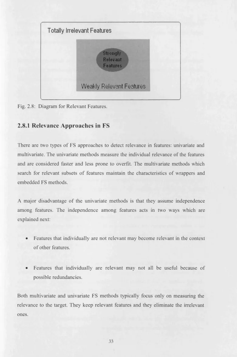
2.5 Unsupervised Feature Relevance
Features are said to be relevant if they are able to give a good description of the elements in a dataset. The objective o f clustering is to group similar elements together (Kaufman and Rousseeuw, 2005) to have a good description of them. Irrelevant features have no influence on forming distinct clusters, but relevant ones do. The similarity of the dataset depends on the correlation o f the features. Most clustering algorithms assume that the features in the dataset are equally important for the clustering task. But contrary to this, different features have different impact in creating clusters. A relevant feature helps to create a cluster while an irrelevant one may affect negatively (Dash and Liu, 2000).
In (Dash et al., 2002) a filter algorithm is presented with an entropy measure to determine the relative relevance o f features. The algorithm ranks the features in terms of relevance taking into account the whole data rather than just individual clusters.
Talavera (2005) developed a wrapper algorithm based on Expectation Maximisation (EM) to estimate the maximum likelihood. This algorithm performs the clustering while at the same time selecting the best subset of features. In a general way this is an iterative procedure which alternates between two steps: the expectation step, and the
maximisation step. An agglomerative algorithm developed by (Talavera, 2005)
considers as relevant features, those ones which present high dependency within the rest of the features. The algorithm at each step merges similar values o f elements among all the features, encouraging cohesive clusters and determining the most relevant features for these clusters.
RIS is a method proposed in (Kailing et al., 2003) that ranks subsets o f features according to their clustering structure. The criterion used to measure the quality of the subsets is a density-based clustering notion o f DBSCAN (Ester et al., 1996). RIS performs a bottom-up navigation through sets of possible subsets accumulating information and ranking them in terms o f importance. Baumgartner and Plant, (2004) proposed an algorithm called SUREING (SUbspaces Relevant For clusterENG). This algorithm measures the relevance o f a subset o f features using a criterion based on its hierarchical clustering structure.
2.6 Statistical Entropy
The concept o f entropy was firstly explained by Boltzman in 1872. The statistical entropy defined in Eq. (2.3) was initially derived only for the number o f possible arrangements in a gas or mixture o f gases (Fast, 1962). However, its validity is so general that in all cases, as yet investigated, it leads to the same results analogous to thermodynamics. The tendency o f entropy to a maximum value according to Eq. (2.3) means nothing else but a tendency to a state o f large number of microstates, i.e. the tendency to a more probable state
S = k \n m (2.5)
The number o f micro-states in the most probable distribution can be written mathematically as S = k h . g max. Applying this equation to a gas only counts those
micro-states in which the gas, macroscopically considered, is distributed uniformity over the available space. On the other hand, when using Eq. (2.3) one only counts the microstates which correspond to non-uniform distributions.
The statistical definition of entropy is often introduced using the connection between probability and entropy. The principle is that the entropy is a function of the number
of different ways in which m, a thermodynamic state, can be realized:
According to classical thermodynamics a reversible state is reached in an isolated system, as soon as the entropy is at the maximum.
2.6.1 Entropy in Data Mining
ID3 is a very popular induction algorithm that uses the entropy measure to find the necessary information to classify instances. ID3 builds a decision tree system selecting the attribute with the minimum entropy in every node to split the tree (Quinlan, 1986). C4.5 is the successor o f ID3 and is one of the most widely used decision tree algorithms. C4.5 has been augmented to C4.5 Rules to convert a decision tree into a rule set (Quinlan, 1995).
Zhu et al., (2010) proposed a model-based approach to estimate the entropy to overcome the sparseness in gene expression data. The entropy on a multivariate normal distribution model o f the data is calculated instead on the data itself.
Lee et al., (2001) presented an algorithm that divides the feature space into good non overlapped decision regions for classification applications. The algorithm divides the feature space using the feature distribution information calculated by Fuzzy entropy.
S = f ( m ) (2.6)
If two systems are considered A and B as one system AB, its entropy is:
Yao et al., (1998) proposed an entropy-based clustering method that calculates the entropy at each data point and selects the one with minimum entropy as the first clusters centre. The algorithm automatically calculates the number and location of the cluster centres. After this, all data points that have similarity are placed, within a threshold, in a chosen cluster centre.
Cheng and Wei (2009) proposed a new entropy clustering method using adaptive learning able to find natural boundaries in datasets and classify similar objects into subsets. The algorithm uses a similarity measure among data points based on the calculation of entropy between two instances (Dash et al., 1997).
Wang (2005) developed algorithms that address the problem of clustering under the framework of possibility theory based on entropy. The algorithm has a number of advantages over other entropy-based approaches such as the ones in (Karayannis, 1994, Li and Mukaidono, 1995, Lorette et al., 2000). The algorithm calculates automatically the number o f clusters by repeatedly merging similar clusters. A resolution parameter is proposed that determines regions o f high density in the dataset.
Jing et al., (2007) extended the k-means algorithm by calculating a weight of importance for each dimension in each cluster. This is achieved using weight entropy in an objective function, that is minimized during the k-means clustering algorithm.
Tsai and Lee (2004) proposed an entropy based approach in neural networks that improves the learning speed, size or recognition accuracy for classification of
structures. Entropy has been successful in determining the architecture of
conventional neural networks in (Bichsel and Seitz, 1989, Cios and Liu, 1992, Lee et al., 1999). To improve the performance o f a classifier Wang and Sontakke (2005) introduced a new packet classification algorithm that hierarchically partitions rule- bases using entropy and hashing.
2.6.2 Entropy as Relevance Measure
In principle, statistical entropy is a technique that can be used to estimate input probabilities by calculating a probability distribution expressed in terms of averages. Statistical entropy has applications in many domains. Started being used in statistical physics to relate macroscopic and measurable properties o f physical systems at atomic or molecular level (Dash and Liu, 2000). In the case of physical systems, entropy is considered a measure o f uncertainty. In communications systems the uncertainty regarding which actual message is to be transmitted is known as the entropy o f the source. In general, entropy depends on the observer. A person may have a different knowledge o f the system from another and thus may calculate a different value for the entropy.
Data has orderly configurations if it has distinct clusters, and disorderly and chaotic configurations otherwise. Entropy is low in orderly configurations, and increases in disorderly configurations (Fast, 1962). Dash et al., (1997) proposed an algorithm to measure the entropy content in a data for several feature projections in order to determine irrelevant features. Jang and Chuen-Tsai, (1995) presented an algorithm based on entropy for UFS. Firstly the data is separated appropriately in clusters. Secondly for each of the clusters the entropy for different sets o f features is computed. At the output, a list of features useful for the description of the data is generated.
Entropy has also been proposed for clustering analysis. For example, Cheng and Wei (2009) proposed a clustering algorithm based on entropy to avoid parameters. The method uses entropy to measure the mean o f the distances between data points and the clusters centres.
2.7 Search Techniques Overview
Because o f the difficulties with optimal strategies, researches have proposed more complex search techniques to find reasonably good features subsets (features in the context o f FS) without exploring all of them. There are plenty of these suboptimal approaches and some o f them are described next:
Exhaustive search is a simple method and the only which guarantees to find the best
subset. It evaluates every possible combination of features. With n candidate variables
there are 2” - 1 subsets to go through, making impossible the evaluation of all of them in a practical amount of time.
Branch and bound is a strategy proposed in (Narendra and Fukunaga, 1997) that
searches only part o f the feature space. The strategy is based on the fact that once a subset S consisting o f more than d variables has been evaluated, we know, thanks to the monotonicity property, that no subset o f it can be better. Thus, unless S excels the currently best known subset S o f target size d, the subsets of S need not be evaluated at all, because there is no way the evaluation result for any o f them could exceed the score o f S . However the algorithm still has an exponential worst case complexity, which may render the approach infeasible when a large number of candidate variables are available.
The Branch and Bound method is not very useful in the wrapper model, because the evaluation function is typically not monotonic, i.e. adding features cannot decrease the accuracy. While methods like the RBABM (Kudo and Sklansky, 2000) are able to relax the requirement slightly, the problem is that typical predictor architectures, evaluated for example using cross-validation, provide no guaranties at all regarding the monotonicity (Guyon et al., 2007).
2.7.1 Sequential Selection Algorithms
SBS {Sequential backward selection) is a sequential pruning of variables introduced
by Marill and Green (1963). This method is the first search technique suggested for variable subset selection. SBS starts with the variable set that consists of all the candidate variables. During one step of the algorithm, remaining variables in the set are considered to be pruned. The results of the exclusion of each variable are compared to each other using certain evaluation function. The step is finished by actually pruning the variable whose removal yields the best results. Steps are taken and variables are pruned until a pre-specified number o f variables are left, or until the results get not good.
SFS {Sequential forw ard selection) is a similar algorithm to SBS proposed in (Whitney, 1971). The algorithm starts with an empty set and continues adding features. In one step each candidate feature that is not yet part of the current set is added, after the set is evaluated. At the end of the step, the feature whose inclusion resulted in the best evaluation is leaved in the current set. The algorithm proceeds until a pre-specifled number of features are selected, or until there is no more improvement in the results.
SFS executes faster than SBS as in the beginning of the search when both methods have a big amount o f possible combinations to evaluate, SFS evaluates much smaller feature sets than SBS. It is true that at the end of the SFS much bigger sets are evaluated than in SBS even that in this stage of the search there are very few combinations left to be considered. SFS evaluates the features in the context of only those that are already included in the subset. Thus, it may not be able to detect a feature that is benefic