Pareto or non-Pareto: Bi-criterion evolution in multi-objective optimization

(1)

Pareto or Non-Pareto: Bi-Criterion Evolution in

Multi-Objective Optimization

Miqing Li, Shengxiang Yang,

Senior Member, IEEE, and Xiaohui Liu

Abstract—It is known that Pareto dominance has its own weak-nesses as the selection criterion in evolutionary multi-objective optimization. Algorithms based on Pareto dominance can suffer from slow convergence to the optimal front, inferior performance on problems with many objectives, etc. Non-Pareto criterion, such as decomposition-based criterion and indicator-based criterion, has already shown promising results in this regard, but its high selection pressure may lead the algorithm to prefer some specific areas of the problem’s true Pareto front, especially when the front is highly irregular. In this paper, we propose a bi-criterion evolution framework of Pareto criterion and non-Pareto criterion, which attempts to make use of their strengths and compensates for each other’s weaknesses. The proposed framework consists of two parts, Pareto criterion evolution and non-Pareto criterion evolution. The two parts work collaboratively, with an abundant exchange of information to facilitate each other’s evolution. Specifically, the non-Pareto criterion evolution leads the Pareto criterion evolution forward and the Pareto criterion evolution compensates the possible diversity loss of the non-Pareto criterion evolution. The proposed framework keeps the freedom on the implementation of the non-Pareto criterion evolution part, thus making it applicable for any non-Pareto-based algorithm. In the Pareto criterion evolution, two operations, population mainte-nance and individual exploration, are presented. The former is to maintain a set of representative nondominated individuals, and the latter is to explore some promising areas which are undeveloped (or not well-developed) in the non-Pareto criterion evolution. Experimental results have shown the effectiveness of the proposed framework. The bi-criterion evolution works well on seven groups of 42 test problems with various characteristics, including those where Pareto-based algorithms or non-Pareto-based algorithms struggle.

Index Terms—Evolutionary multi-objective optimization, Pareto criterion, non-Pareto criterion, bi-criterion evolution.

I. INTRODUCTION

T

HE area of multi-objective optimization has developed

rapidly over the past few decades, reflecting the need of simultaneously dealing with multiple objectives in real-world problems. Unlike global optimization in which there is often a single optimal solution, multi-objective optimization involves a set of Pareto optimal solutions. Evolutionary algorithms

Manuscript received December 5, 2014; revised April 8, 2015 and Septem-ber 18, 2015; accepted NovemSeptem-ber 23, 2015. This work was supported in part by the Engineering and Physical Sciences Research Council (EPSRC) of U.K. under Grant EP/K001310/1, National Natural Science Foundation of China under Grant 71110107026 (Major International Joint Research Project) and Grant 61273031, and EPSRC Industrial Case under Grant 11220252 (Corresponding author: Shengxiang Yang).

M. Li and X. Liu are with the Department of Computer Science, Brunel University London, Uxbridge, Middlesex UB8 3PH, U. K.

S. Yang is with the School of Computer Science and Informatics, De Montfort University, Leicester LE1 9BH, U. K. (e-mail: [email protected]).

(EAs) have shown high practicability in solving such multi-objective optimization problems (MOPs). Their population-based search aims at finding a finite-size set of well-converged, well-distributed solutions, each representing a unique trade-off among the objectives.

In evolutionary multi-objective optimization (EMO), the selection criterion of individuals in the population plays a key role. Since the output of an EMO algorithm for a MOP is a set of Pareto non-dominated solutions, Pareto dominance naturally becomes a viable criterion to select individuals during the evolutionary process. Pareto dominance reflects the weakest assumption about the preference of a decision maker; an

individual x is said to Pareto dominate an individual y if

it is as good as y in all objectives and better in at least

one objective. This criterion, however, fails to distinguish between individuals when they have their own advantage in different objectives of a MOP. In this case, most Pareto-based EMO algorithms, such as the nondominated sorting genetic algorithm II (NSGA-II) [14], introduce the density information of individuals in the population to further rank them, serving the purpose of evolving towards different parts of the problem’s true Pareto front.

Despite its popularity in the EMO community, the Pareto criterion (PC) or a Pareto-based algorithm is known to suffer from some drawbacks, such as slow convergence to the optimal front [59], no information of quantitative difference between two individuals [5], [67], and inferior performance on MOPs with a complex Pareto set (PS) [44] or a high-dimensional objective space [31], [64]. Recently, some non-Pareto selection criteria have been shown to be promising in tackling MOPs. Typically, they convert an objective vector into a scalar value, thus providing a totally-ordered set of individuals in the population. Compared with the PC, such criteria have clear advantages, e.g., providing higher selection pressure towards the true Pareto front [7], [35], [39] and being easier to work with local search techniques stemming from global optimization [5], [43].

The indicator-based EA (IBEA) [78] and decomposition-based multi-objective EA (MOEA/D) [71] are two represen-tative examples in using the non-Pareto criterion (NPC) to deal with MOPs. IBEA adopts a performance indicator to optimize a desired property of the evolutionary population, and MOEA/D decomposes a MOP into a set of scalar sub-problems and handles them collaboratively with the aid of the information from their neighbors. These two algorithms have laid the foundation for much state-of-the-art work to date, leading to indicator-based and decomposition-based criteria, respectively, which, along with the PC, have become three

(2)

mainstream selection criteria in the EMO area [12], [73]. However, an NPC also comes with some shortcomings. Ide-ally, the outcome of an EMO algorithm is a set of uniformly-distributed solutions on the whole true Pareto front. These solutions are Pareto optimal and are supposed to be incompara-ble in terms of proximity (convergence). But, most non-Pareto criteria, which typically provide higher selection pressure than the PC, make Pareto optimal solutions comparable, completely [13], [78] or partly [17], [42]. In such criteria, different parts of the true Pareto front are treated differently, e.g., the knee and

border of the front being usually preferred by thehypervolume

-based criterion [3], [55]. In this way, even some Pareto optimal solutions may be eliminated during the evolutionary process as they are not in favor with the criterion used, which can result in the final solutions distributed “regularly”, but not uniformly along the true Pareto front.

Note that the decomposition-based criterion seems to be exempt from the above problem since it, by using a set of weight vectors, specifies multiple search directions towards different parts of the true Pareto front. One key issue in decomposition-based EMO techniques, however, is how to maintain the uniformity of intersection points of the spec-ified search directions and the problem’s true Pareto front. Uniformly-distributed weight vectors cannot guarantee the uni-formity of the intersection points. In fact, it is very challenging for decomposition-based algorithms to access a set of the well-distributed intersection points for any MOP, in particular in real-world scenarios where the information of a problem’s true Pareto front is often unknown. Although much effort has been made on this issue recently [2], [16], [21]–[24], [37], [54], [68], it is still far from being resolved completely, especially when facing a MOP with a highly irregular optimal front (e.g., a discontinuous or degenerate front).

Given the above, one question could arise: is it possible to develop an algorithm of synthesizing the Pareto and non-Pareto selection criteria, which makes full use of their advan-tages as well as effectively avoiding their disadvanadvan-tages? In this paper, we make an attempt along this line and present a bi-criterion evolution (BCE) framework for MOPs. In BCE, the PC and NPC work collaboratively, trying to guide the popula-tion evolving fast towards the optimal front and simultaneously maintain individuals’ diversity during the evolutionary process. BCE manipulates two evolutionary populations, called the NPC population and the PC population, respectively, each of which is associated with one criterion. The NPC population steers the PC population searching towards the optimal front, while the PC population compensates the possible diversity loss of the NPC population by exploring some undeveloped (or not well-developed), but potentially promising regions in the objective space. The two populations communicate with each other in a generational manner; once one population produces good individuals, the other is able to apply them directly within its search process.

BCE keeps it free on the design of the NPC evolution part, thus making the framework applicable for any non-Pareto-based EMO algorithm in the area. Effort of BCE is primarily on the PC evolution part. In the PC evolution, an individual exploration operation, coupled with a novel

population maintenance strategy, is proposed to adaptively allocate resources (search effort), based on the information contrast between the current states of the two evolution parts. The rest of this paper is organized as follows. Section II explains the motivation of the proposed approach. Section III is devoted to the description of BCE, including the basic algo-rithmic framework, the population maintenance and individual exploration operations, and the analysis of the algorithm’s time complexity. Section IV experimentally verifies the proposed BCE framework, based on its implementation with three rep-resentative non-Pareto-based algorithms. Further investigation and discussion of BCE’s behavior are given in Section V and Section VI, respectively. Finally, Section VII draws the conclusions of the paper.

II. MOTIVATION ANDRELATEDWORK

Over the past few years, non-Pareto criteria have demon-strated their success in dealing with many challenging MOPs, such as a MOP with a huge number of local Pareto fronts [17], with a complex PS [44], [70], or with a high-dimensional objective space [32], [48], [64]. They typically provide higher selection pressure than the Pareto criterion, by either modi-fying the traditional Pareto dominance relation (such as the

ǫ-dominance [17], [42], [63], fuzzy-based dominance [26],

and dominance area control [56]) or introducing a quantitative individual comparison criterion (such as the distance-based criterion [50], [66], indicator-based criterion [8], [39], [78], and decomposition-based criterion [51], [71]).

However, non-Pareto criteria also suffer from problems, e.g., in terms of maintaining individuals’ diversity (especially uniformity) in the population. In general, the ideal output of an EMO algorithm, in the absence of any preference information, is a set of uniformly-distributed nondominated solutions over the whole true Pareto front. This means that the comparison between the Pareto optimal solutions should be solely based on their density information. But, this is not the case in non-Pareto criteria where the non-Pareto optimal solutions could be ranked, depending not only on their density but also on their position in the population as well as the shape of the true

Pareto front. For example, the ǫ-dominance criterion [42] is

likely to eliminate boundary individuals of the population [27], [48]. Some indicator-based criteria, like the hypervolume [75]

andR2[9], prefer the knee region of the true Pareto front [19],

[55]. The algorithms based on the decomposition criterion search towards a set of points intersected by the specified search directions and the true Pareto front, but struggle to maintain the uniformity of these intersection points when the front is highly irregular [24], [37], [54].

Next, we give an empirical example to show the failure of a non-Pareto-based algorithm in providing a set of representative solutions. Fig. 1 shows the results with respect to one typical

run1 _{of a popular decomposition-based algorithm, MOEA/D}

[71] with the Tchebycheff scalarizing function2 _{(denoted as}

1_{The parameter setting in the run is the same as in the experimental studies,}

described in Section IV.

2_{In order to obtain more uniform solutions, in the Tchebycheff scalarizing}

function, “multiplying the weight vectorwi” in the original MOEA/D+TCH

[71] is replaced by “dividingwi”, as suggested and practiced in recent studies

(3)

(a) (b) (c) (d)

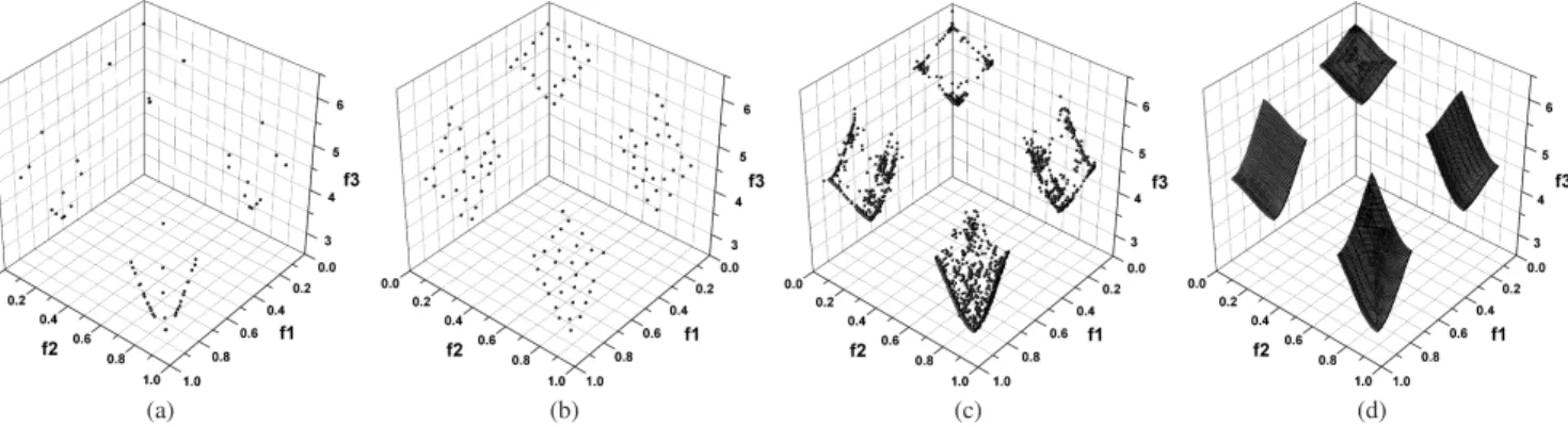
Fig. 1. An empirical example of the failure of an NPC in both diversity maintenance and search, where the results are obtained with respect to one run of

MOEA/D+TCH on the problem DTLZ7. (a) Solution set maintained by the original criterion of MOEA/D+TCH; (b) Solution set maintained by the criteria of Pareto dominance and density; (c) Nondominated set of all solutions produced in the run; (d) True Pareto front.

MOEA/D+TCH), on a discontinuous test problem DTLZ7 [18]. The final solutions obtained by MOEA/D+TCH are plotted in Fig. 1(a). For contrast, Fig. 1(b) gives the final result of the solution set maintained by the criteria of Pareto-based algorithms (i.e., solutions being tested first by their

Pareto dominance relation and then by their density3_{) in this}

run of MOEA/D+TCH. That is, an external archive set is added in the algorithm to store well-distributed nondominated solutions produced throughout the whole evolutionary process. In addition, the nondominated set of all solutions produced in this run is given in Fig. 1(c).

As can be seen from Figs. 1(a) and (c), MOEA/D+TCH fails to select a set of diverse solutions from all the solutions produced in the whole evolutionary process. In contrast, the se-lection criteria of Pareto-based algorithms, which consider the Pareto dominance relation and density of candidate solutions, can make the algorithm’s output representative, as shown in Fig. 1(b). On the other hand, the deficiency of the algorithm in diversity maintenance also has a detrimental effect on its search ability. To explain this, the true Pareto front of the problem is added in Fig. 1(d) for the comparison between the real optimal solutions and the solutions produced during the evolutionary process. From Figs. 1(c) and (d), it can be observed that there exist several large pieces of unexplored regions in MOEA/D+TCH’s search process. This occurrence can be attributed to the fact that the selection operation in this non-Pareto algorithm is always around some particular points (cf. Fig. 1(a)) at each generation, thus leading individuals’ exploration to concentrate only on some specific regions of the objective space.

The above problems of non-Pareto criteria are precisely the underlying motivation of our study. In this paper, we introduce a BCE framework of Pareto and non-Pareto criteria, in order to use their strengths and compensate for each other’s weaknesses.

It is worth pointing out that the combination of NPC and

PC is not uncommon in EMO. For example, Ishibuchi et

al. [33] combined the Pareto-based algorithm NSGA-II with

the weighted sum criterion to probabilistically pick out solu-tions in both mating and environmental selection processes.

3_{Here individuals’ density is estimated by the method in BCE, described}

in Section III-B.

Al Moubayedet al. [1] used a decomposition-based criterion

to select the leaders in multi-objective particle swarm opti-mization (PSO) and introduced the crowding distance to main-tain the diversity of nondominated solutions in the decision and objective spaces. Deb and Jain [16] proposed a hybrid EMO algorithm, NSGA-III, which uses the Pareto nondominated sorting to develop convergence and the decomposition-based criterion to maintain diversity during the evolutionary process. On the other hand, some studies in the literature adopted multiple archives (or populations) to separately promote con-vergence and diversity during the evolutionary process. Wang

et al.[65] developed a two-archive many-objective algorithm, with one archive being driven by an indicator-based criterion

and the other being maintained by an Lp-norm-based

dis-tance criterion. Z˘avoianu et al. [69] presented a hybrid

co-evolutionary algorithm with three populations, each one asso-ciated with a classic algorithm, i.e., SPEA2 [74], differential

evolution [41], and a decomposition-based algorithm. Cai et

al. [10] proposed a hybrid EMO algorithm for combinatorial

MOPs, by using a decomposition-based strategy to guide its internal population and a domination-based sorting technique to maintain the external archive. In addition, the idea of having separate archives has also been used in multi-objective scatter search, where the reference set is split into two subsets that promote convergence and diversity, respectively. In multi-objective scatter search algorithms, Pareto dominance and decomposition criteria are often used in the convergence-promoting subset, and distance-based criteria in the diversity-promoting subset [6], [49], [52].

An important difference between the proposed BCE and existing hybrid EMO algorithms with multiple criteria and/or multiple archives is that BCE takes advantage of the infor-mation contrast between the evolutionary populations based on distinct selection criteria, thus making the search focused on promising regions in terms of both Pareto and non-Pareto criteria. Another clear difference is that BCE is a general framework rather than a specific algorithm, and it can work with any non-Pareto EMO algorithm.

III. BI-CRITERIONEVOLUTION

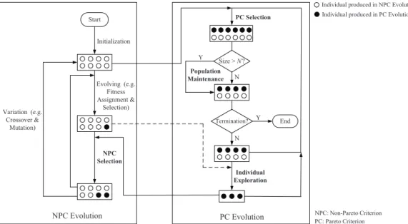
Fig. 2 gives the overall framework of BCE. As shown, BCE consists of two evolution parts, NPC evolution and PC

(4)

Initialization Evolving (e.g. Fitness Assignment & Selection) Size > N? Population Maintenance Y N Termination? End Start Y N Individual Exploration NPC Selection Variation (e.g. Crossover & Mutation) PC Selection

NPC Evolution PC Evolution NPC: Non-Pareto Criterion PC: Pareto Criterion

Individual produced in NPC Evolution Individual produced in PC Evolution

Fig. 2. Overall framework of bi-criterion evolution.

evolution. BCE keeps the freedom on the implementation of the NPC evolution part – any non-Pareto EMO algorithm can be directly embedded, with all components (population setting, individual initialization, fitness assignment, selection, varia-tion, etc.) remaining unchanged. The only newly-introduced operation is that the population for the next-generation evo-lution (the bottom box) is comprised of individuals which are selected from itself and newly produced individuals in the PC evolution part (called the NPC selection). Note that the two arrow lines (both starting from the bottom box) in the NPC evolution are different. The exterior line is to carry out the variation operations (e.g., crossover and mutation) on the bottom-box population and put the resulting population in the top box. The interior line is to combine the bottom-box population with the top-box one and then perform the selection operation on this mixed population (by means of fitness) to form the middle-box population.

For the PC evolution part, the manipulated population (i.e., the PC population) only preserves the Pareto nondominated solutions produced in both NPC and PC evolution, thereby having a varying size. When the size of the PC population is larger than a predefined threshold, a population maintenance operation will be implemented to eliminate some poorly distributed individuals. If here the termination condition is satisfied (e.g., reaching a preset number of evaluations), the evolution ends with the PC population as the final output. Otherwise, an individual exploration operation is implemented to explore some promising individuals in the PC population, bearing the evolutionary information from the NPC popula-tion.

In BCE, the two populations share and exchange informa-tion frequently, but evolve based on their own criterion. Any new individual (wherever it is produced) will be considered in both sides of BCE to see if it could be preserved in their own population. In general, the PC population can be regarded as a good complement to the NPC population. It is able to not only

preserve representative Pareto nondominated solutions which could be eliminated in the NPC evolution, but also reflect the current status of the NPC evolution by the information contrast between the two populations.

Next, we describe key operations of BCE. They are the PC and NPC selection, population maintenance, and individual exploration.

A. PC Selection and NPC Selection

As their names suggest, the PC and NPC selections are to select individuals (from the considered population and the newly produced individuals) according to the PC and NPC, respectively. The PC selection is implemented by directly picking out the Pareto nondominated individuals from the mixed set of the PC population and new individuals produced in both the NPC and PC evolutions .

The NPC selection, in general, can be simply implemented by the environmental selection operation of the embedded non-Pareto-based algorithm. For example, in the NPC selection of BCE-IBEA (i.e., BCE with IBEA embedded into its NPC evolution part), the resulting NPC population is comprised of the individuals with the highest fitness with respect to the considered criterion (indicator) in the mixed set of the NPC population and the new individuals from the PC evolution. But, this is impracticable for some algorithms where the survival of a newly produced individual is relevant to the information from its parent(s), such as MOEA/D. This is because the candidate individuals in the NPC selection are from different evolution parts, without being in the parent-child relationship. For these algorithms, the NPC selection compares each individual from the PC evolution with all the members of the NPC population. If an individual from the PC evolution performs better than one or more population members with respect to the considered criterion, then it replaces one of them (chosen at random); otherwise, it is discarded. Algorithm 1 gives the procedure of the NPC selection.

(5)

Algorithm 1 N P Cselection(Q, T)

Require: Q (non-Pareto criterion population), T (newly produced individual set in the Pareto criterion evolution part),label(type of the environmental selection in the embedded non-Pareto algorithm)

1: label←SelectionT ype()/∗_Return₁_{if the survival of a newly} produced individual is irrelevant to its parent(s) in the selection process of the non-Pareto algorithm; otherwise, return0∗_/ 2: iflabel= 1then

3: Q←EnvironmentalSelection(Q, T)

/∗ _Select _|_Q_|_{individuals with the highest fitness with} respect to the considered non-Pareto criterion fromQ∪T ∗_/

4: else

5: for allt∈T do

6: Z← ∅

7: for allq∈Qdo

8: if t is better than q with respect to the considered criterionthen 9: Z←Z∪q 10: end if 11: end for 12: ifZ6=∅then 13: z←Random(Z)

/∗_{Select one individual from}_Z _{at random}∗_/

14: Q←Q\z 15: Q←Q∪t 16: end if 17: end for 18: end if 19: return Q B. Population Maintenance

In the PC evolution part, the population preserves the Pareto nondominated individuals produced during the whole search process and has a varying size. When the size of the population exceeds a predefined capacity, population maintenance will be activated to truncate some of its individuals with poor distri-bution. It is known that an effective population maintenance operation can maintain a set of representative individuals, which is independent of the properties of the problem (e.g., the number of objectives and the shape of the true Pareto front). In this paper, we present a niche-based approach, attempting to preserve a set of representative individuals for any MOP.

Niching is a class of popular diversity maintenance tech-niques in the EA field. Originating from the idea of shar-ing resources, nichshar-ing can be used to measure individuals’ crowding degree (density) in the population. Here, we estimate the crowding degree of an individual by considering both the number and location of the individuals in its niche.

Specifically, the crowding degree of an individual p in the

population P is defined as follows:

D(p) = 1− Y q∈P,q6=p R(p, q) (1) R(p, q) = d(p, q)/r , if d(p, q)≤r 1, otherwise (2)

where d(p, q) denotes the Euclidean distance between

indi-viduals pand q, and r is the radius of the niche (its setting

will be explained later). Note that the scale of the problem’s objectives could be highly different and this will affect the

estimation of individuals’ crowding degree here. To avoid this kind of problem, in BCE all the objectives will be normalized (with respect to their minimum and maximum values in the population) when the considered operation involves the integration of multiple objectives.

Next, we give some explanations of the proposed crowding degree estimation method.

• The crowding degree of an individual is in the range

[0,1], with a lower value being preferable. An individual

having the crowding degree 0 means that there is no

other individual in its niche. On the other hand, duplicate

individuals have the highest crowding degree1, regardless

of the distribution of other individuals in their niche.

• The crowding degree of an individual is determined by

the number of its neighbors (i.e., the individuals in its niche) and the distance between it and these neighbors. Individuals having more neighbors or closer distance to their neighbors are likely to obtain a higher (worse) crowding degree.

• The crowding degree of an individual is influenced more

by its closer neighbor(s). For example, considering two

individualspandq, let both of them have two neighbors

and the sum of the distance to their own neighbors be the

same (say0.2 and0.8 forpand0.4 and0.6forq).

Ac-cording to the definition,p, which has a shorter distance

(0.2) to its closer neighbor, will have a higher crowding

degree thanq(1−0.16/r2

= 0.84>1−0.24/r2

= 0.76,

assumingr= 1.0here). Actually, even ifphas only one

neighbor (closer one), its crowding degree is still higher

than that ofq (1−0.2/r = 0.8>1−0.24/r2_{= 0}_.₇₆

). This means that an individual which has very close neighbor(s) will be assigned a high crowding degree no matter how far it is from other individuals in the population. This is in line with the target of developing the diversity of individuals.

One crucial issue in the proposed crowding degree estimator is the setting of the niche radius, which determines the number of neighbors as well as their location in the niche. Unlike some niching techniques where it is fixed and/or set by the user, the niche radius in the proposed estimator is determined by the evolutionary population. We consider the average of the

distance from all the individuals to theirkth nearest individual

in the population as the radius, attempting to enable most of the individuals to have one or several neighbors in their niche.

Here,kis set to3. The reason of this setting will be explained

in detail in the discussion section of the paper (Section VI) Based on the crowding degree of individuals in the popu-lation, the truncation operation can be simply implemented. First, the individual which has the highest crowding degree is removed; if there are several individuals with the highest crowding degree, the tie will be split randomly. Then, the crowding degree of the individuals who are neighbors of the removed individual (i.e., in its niche) is renewed, and again the current most crowded individual is found and removed. This process is repeated until a predefined population size is achieved. Overall, the proposed method iteratively removes crowded individuals and thus leaves a representative

(6)

popula-tion, and this can also be observed in the example of Fig. 1 (see Figs. 1(b) and (c)).

C. Individual Exploration

In BCE, the NPC evolution generally has higher selection pressure than the PC evolution and may prefer partial area(s) of the true Pareto front sometimes. This may cause repeating search on some particular regions of the objective space. The individual exploration operation in this section aims to cover

this issue. It attempts to explore somepromisingindividuals in

the PC population which have been eliminated, are not well-developed, or are even unvisited in the NPC evolution. This exploration is adaptive, based on the information comparison between the two evolutionary populations. If the NPC popu-lation has been found to be well distributed, little exploration will be made; otherwise, much exploration will be made around those promising individuals.

Now, a key question may arise – what individuals are promising and need to be explored? Since the PC population is comprised of a set of representative nondominated individuals, it generally performs well in both convergence and diversity. Nevertheless, it is unnecessary to explore the whole PC population as some of its individuals may already be well explored in the NPC evolution. Such individuals are preferred by the considered NPC and there may be many individuals in the NPC population located around the regions where such individuals reside.

In view of this, we consider two kinds of individuals out of the whole PC population: 1) individuals whose niche has

no NPC individual4 and 2) individuals whose niche has only

one NPC individual. The first kind of individuals is clearly not preferred by the considered NPC. Exploring them means to probe into undeveloped regions in the NPC evolution. The niches in which the second kind of individuals resides correspond to low density regions of the NPC population. Exploring them means to probe into the regions which are not well developed in the NPC evolution, but may be potentially promising since they still have individual(s) existing in both the NPC and PC populations after (iterative) selection based on the non-Pareto and Pareto criteria, respectively.

Algorithm 2 gives the main procedure of individual explo-ration. As shown, the algorithm can primarily be divided into two parts. One is to determine which individuals in the PC population will be explored (Steps 3–13) and the other is to carry out the exploration on those individuals (Steps 15–18). In the proposed framework, the variation operation (Step 16) is not fixed and can be freely specified by users. It can be the same with what is in the NPC evolution (as done in our experimental studies), be chosen from other existing variation operators, or even be directly designed for the exploration here. In addition, note that in different variation operators the number of parent individuals may be different. For a variation operator with only one parent (like mutation), the explored individual is applied directly. For a variation operator with two or more parents (like crossover), the explored individual is

4_{For brevity, individuals in the NPC and PC populations are denoted as}

NPC and PC individuals, respectively.

Algorithm 2 Exploration(P, Q)

Require: P (Pareto criterion population), Q (non-Pareto criterion population),S (set of the individuals to be explored), T (set of newly produced individuals)

1: S← ∅

2: r←Radius() /∗_{Determine the size of the niche}∗_/ 3: for allp∈P do

4: count←0 /∗_For record-ing the number of the NPC individuals in the niche ofp∗_/ 5: for allq∈Qdo

6: ifd(p, q)≤r then

7: count←count+ 1 /∗_When_q_{is in the niche of}_p∗_/ 8: end if

9: end for

10: ifcount= 0orcount= 1 then

11: S←S∪p 12: end if 13: end for 14: T ← ∅ 15: for alls∈S do 16: s′_←_{V ariation(s)} 17: T ←T∪s′ 18: end for 19: return T

considered as one parent (or the primary parent in the operator, e.g., in differential evolution) and the remaining parent(s) will be selected randomly from the PC population.

In Step 2 of Algorithm 2, the radius of the considered niche is calculated. The niche range is an important factor in individual exploration, which, together with the distribution of NPC individuals, determines how many individuals will be explored in the PC population. A small enough niche is likely to lead all PC individuals to be explored, and a large enough niche can cause none of them to be done. Here, we introduce a variable niche, whose range varies with the size of the PC population.

The PC population only preserves nondominated individu-als, and its size can reflect the role of the Pareto dominance criterion during the evolutionary process. A small population size means that Pareto dominance can provide sufficient selec-tion pressure to eliminate poorly-performed individuals. This usually happens in the initial stage of the evolution. At this time, the population maintenance operation is not activated, and the PC population which stores all nondominated individu-als produced in both the NPC and PC evolutions represents the best individuals found so far. Therefore, it is desirable to put more effort to explore it. With the progress of the evolution, more and more individuals are produced and Pareto dominance may gradually fail to provide sufficient selection pressure. When newly produced nondominated individuals significantly exceed the remaining slots of the population capacity, the PC evolution will slow down. At this time, it is beneficial to make relatively less exploration on the PC population, thus leading to more resources possessed by the NPC evolution which generally has high selection pressure. Given the above, the radius of the niche is determined as follows:

r= (N′/N)×r0 (3)

(7)

(a) MOEA/D+TCH (b) BCE-MOEA/D+TCH

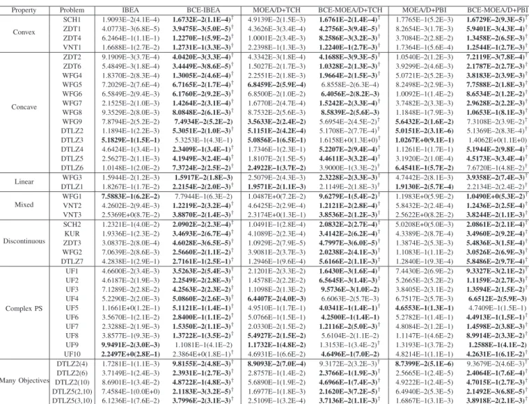
Fig. 3. The nondominated set of all the solutions produced in one run of

MOEA/D+TCH and BCE-MOEA/D+TCH on DTLZ7, respectively.

denotes the actual size of the PC population before the

truncation, andr0 is the basic niche radius, calculated in the

same way as in the population maintenance operation. In BCE, individual exploration in the PC evolution in-evitably competes with the variation operation in the NPC evolution for limited computational resources (i.e., function evaluations). Given a fixed computational budget, the number of individuals explored directly affects the evolutionary level of the NPC population. However, it is worth noting that individual exploration here is adaptive, depending on the current evolutionary status of the NPC population. When the NPC population has diversity loss (like the case in Fig. 1(a) where the decomposition-based criterion struggles to maintain diversity), intensive exploration will be made. When the pop-ulation has been found to be well distributed, little or even no exploration will be done; for instance, for the test function DTLZ2 [18] the decomposition-based evolutionary population can work very well and thus no individual is explored in the PC population (this will also be empirically presented in Section V-B).

Finally, Fig. 3 gives the comparative results of the origi-nal MOEA/D+TCH (i.e., Fig. 1(c)) and BCE-MOEA/D+TCH (BCE with MOEA/D+TCH embedded into its NPC evolution part) by plotting all of their nondominated individuals pro-duced in one run. In contrast to MOEA/D+TCH’s solutions which are located around some specific regions, the solutions produced by BCE-MOEA/D+TCH nearly cover the whole optimal space. This difference can be fully attributed to the individual exploration operation in the PC evolution part of the algorithm, which conducts the search on some undeveloped (or not well-developed) regions in the NPC evolution.

D. Computational Complexity of One Generation of BCE

BCE’s computational cost comes from two parts, the NPC evolution and the PC evolution. For simplicity, let both parts

have the population size (capacity)N. For the time complexity

of the NPC evolution, there are two possible situations, de-pending on the selection operation in the embedded non-Pareto algorithm. When the survival of an individual is determined by its fitness in the population (like in IBEA), the NPC selection is implemented in the same way as the individual selection in the embedded algorithm (cf. Section III-A). In this case, the

NPC evolution has the same time complexity as the embedded

algorithm (denoted asC). On the other hand, when the survival

of an individual is relevant to the information from its parents (like in MOEA/D), the NPC selection is implemented by comparing the individuals produced in the PC evolution with

the members of the NPC population. This requires O(N2₎

comparisons at most. Hence, the time complexity of the NPC

evolution in this situation isCorO(N2₎

, whichever is larger. The computational cost of the PC evolution part is de-termined by three operations, the PC selection, population maintenance, and individual exploration. The PC selection, which identifies nondominated individuals from a population

with 3N members at most, requires O(mN2₎

comparisons

[14], wheremis the number of objectives. In the population

maintenance, the Euclidean distance between each pair of individuals in the population is first calculated, which

re-quires O(mN2₎

computations. Then, determining the niche

radius requires O(N2₎

computations, in which finding the

kth smallest distance (k= 3) for an individual needsO(N)

comparisons. Thereafter, the crowding degree estimation and the population truncation are sequentially implemented. Both

requires O(N2

) computations (or comparisons). It is worth

mentioning that in the population truncation we only need to update the crowding degree of the neighbors of the removed individual (i.e., the individuals which is in the same niche of the removed individual). In general, the niche of an individual

only has a few individuals (independent of N) due to the

setting of the radius (namely, the average distance from all

individuals in the population to their3rd nearest individual). In

the individual exploration, the Euclidean distance between the individuals and the radius of the niche are also calculated first,

which require O(mN2₎

and O(N2₎

computations, respec-tively. Then, determining which individuals in the population

will be explored requiresO(N2₎

comparisons (Steps 3–13 in Algorithm 2). Finally, carrying out the exploration operation

on the selected individuals requires O(N) computations at

most. Therefore, the total time complexity of the PC evolution

isO(mN2

).

To sum up, the overall computational complexity of one

generation of BCE is bounded by C orO(mN2₎

, whichever

is larger, where C is the computational complexity of the

embedded non-Pareto algorithm.

IV. PERFORMANCEVERIFICATION OFBCE

The proposed framework is verified by embedding non-Pareto EMO algorithms into its NPC evolution part and comparing these non-Pareto algorithms with the resulting BCE algorithms. We consider two representative non-Pareto-based algorithms, IBEA [78] and MOEA/D [44], which lead the evolution via the indicator-based criterion and decomposition-based criterion, respectively. In MOEA/D, two scalarizing functions Tchebycheff (TCH) and penalty-based boundary intersection (PBI) are commonly used in the literature, and both are included in our experiments in view of their good performance for different MOPs [16], [32], [44], [47]. Note that MOEA/D used here is sourced from [44] rather than from its original paper [71]. This improved version can largely

(8)

TABLE I

SETTINGS AND PROPERTIES OF TEST PROBLEMS.mANDdDENOTE THE NUMBER OF OBJECTIVES AND DECISION VARIABLES,RESPECTIVELY

Problem m d Properties Problem m d Properties Problem m d Properties

SCH1 2 1 Convex WFG7 2 22 Concave, Biased UF2 2 30 Convex, Complex PS

SCH2 2 1 Discontinuous WFG8 2 22 Concave, Nonseparable, Biased UF3 2 30 Convex, Complex PS KUR 2 3 Discontinuous WFG9 2 22 Concave, Nonseparable, Deceptive, Biased UF4 2 30 Concave, Complex PS

ZDT1 2 30 Convex VNT1 3 2 Convex UF5 2 30 Linear, Discrete, Complex PS

ZDT2 2 30 Concave VNT2 3 2 Mixed UF6 2 30 Linear, Discontinuous, Complex PS ZDT3 2 30 Discontinuous VNT3 3 2 Mixed, Degenerate UF7 2 30 Linear, Complex PS ZDT4 2 10 Convex, Multimodal DTLZ1 3 7 Linear, Multimodal UF8 3 30 Concave, Complex PS ZDT6 2 10 Concave, Multimodal, Biased DTLZ2 3 12 Concave UF9 3 30 Linear, Discontinuous, Complex PS WFG1 2 22 Mixed, Biased DTLZ3 3 12 Concave, Multimodal UF10 3 30 Concave, Complex PS WFG2 2 22 Convex, Discontinuous, Nonseparable DTLZ4 3 12 Concave, Biased DTLZ2(4) 4 13 Concave WFG3 2 22 Linear, Degenerate, Nonseparable DTLZ5 3 12 Concave, Degenerate DTLZ2(6) 6 15 Concave WFG4 2 22 Concave, Multimodal DTLZ6 3 12 Concave, Degenerate, Biased DTLZ2(10) 10 19 Concave WFG5 2 22 Concave, Deceptive DTLZ7 3 22 Mixed, Discontinuous, Multimodal DTLZ5(2,10) 10 19 Concave, Degenerate WFG6 2 22 Concave, Nonseparable UF1 2 30 Convex, Complex PS DTLZ5(3,10) 10 19 Concave, Degenerate

enhance the diversity of the population, by allowing parent individuals to be selected from the whole population as well as setting a limit of the maximal number of individuals replaced by a newly produced child individual. In addition, in the TCH scalarizing function, we replace “multiplying the weight vector” with “dividing it” for obtaining more uniform individuals, as pointed out in [16], [37]. Overall, the intention that we consider this version of MOEA/D is to verify the effectiveness of BCE even when the considered non-Pareto algorithms already work fairly well in terms of diversity maintenance on most MOPs.

A comprehensive set of 42 MOPs are introduced in the experiments. These test problems, which are widely used in the area, have various properties, such as having a con-vex, concave, mixed, discontinuous or degenerate true Pareto front, having a multimodal, biased or deceptive search space, and/or having strong-linkage decision variables. They certainly include some MOPs where non-Pareto algorithms generally work well, like a MOP with a linear (or fairly regular) true Pareto front, and also have some where the algorithms may encounter difficulties, like a MOP with a discontinuous (or highly irregular) true Pareto front. Table I summarizes the properties and configuration of these MOPs. All the problems are configured as described in their original papers [18], [28], [57], [62], [70], [76].

To compare the performance of the algorithms, two widely-used quality indicators, the inverted generational distance (IGD) [16], [71] and hypervolume (HV) [75], are considered as they can provide a combined information of convergence and diversity of a solution set. IGD measures the average Euclidean distance from uniformly distributed points along the whole true Pareto front to their closest solution in the obtained solution set, and a smaller value is preferable. HV calculates the volume of the objective space between the obtained solution set and a specified reference point, and a larger value is preferable.

In the calculation of HV, two crucial issues are the scaling of the search space [20] and the choice of the reference point [3]. Since the objectives in the considered test problems take different ranges of values, we standardize the objective value of the obtained solutions according to the range of the problem’s true Pareto front. Following the recommendation in [34], the reference point is set to 1.1 times the upper bound of

the true Pareto front (i.e.,r= 1.1m_{) to emphasize the balance}

TABLE II

POPULATION SIZE AND FUNCTION EVALUATIONS IN THE EXPERIMENTS

Test Problems Population Size Function Evaluations

2-Obj. UF 600 300 000

3-Obj. UF 1 000 300 000

General 2-Obj. MOPs 100 25 000 General 3-Obj. MOPs 105 30 000

4-Obj. MOPs 220 100 000

6-Obj. MOPs 252 100 000

10-Obj. MOPs 220 100 000

between proximity and diversity of the obtained solution set. Note that solutions that do not dominate the reference point are discarded (i.e., solutions that are worse than the reference point in at least one objective contribute zero to HV).

All the results presented in this study are obtained by executing 30 independent runs for each algorithm. For a fair comparison, all the algorithms have the same size (or capacity) of the population (for BCE, this refers to both the NPC and PC populations) and the same number of function evaluations on each problem. Table II lists the settings of the population size and function evaluations for all the test problems in the experiments. For the UF functions from the CEC2009 competition [70], the population size and function evaluations are specified the same as in their original report [72]. For other MOPs, we used a smaller population size and fewer function evaluations as they are generally easier than the UF functions. Like most existing studies, the number of function evaluations is set to 25,000 and 30,000 for 2- and 3-objective MOPs, respectively. Note that in MOEA/D the population size corresponds to the number of weight vectors and the algorithm cannot generate uniformly distributed weight vectors at an arbitrary number. So, we set the population size consistent with the number of the uniformly generated weight vectors in MOEA/D. That is 100, 105, 220, 252 and 220 for the 2-, 3-, 4-, 6- and 10-objective MOPs, respectively. In addition, given that many-objective problems often bring bigger challenges for EMO algorithms than MOPs with 2 or 3 objectives [53], we assign them a larger population size and more function evaluations, following the practice in [46].

Parameters need to be set in the considered algorithms. According to the study in [70], the size of the neighborhood, the probability of parent individuals selected from the neigh-borhood, and the maximum number of replaced individuals

(9)

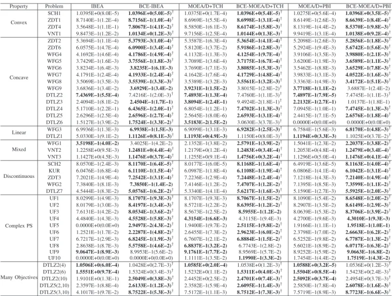
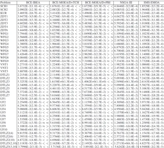
TABLE III

IGDRESULTS(MEAN ANDSD)OF THE THREE GROUPS OF PAIRED ALGORITHMS. THE BETTER MEAN FOR EACH CASE IS HIGHLIGHTED IN BOLDFACE

Property Problem IBEA BCE-IBEA MOEA/D+TCH BCE-MOEA/D+TCH MOEA/D+PBI BCE-MOEA/D+PBI Convex

SCH1 1.9093E–2(4.1E–4) 1.6732E–2(1.1E–4)† 4.9139E–2(1.5E–3) 1.6761E–2(1.4E–4)† 1.7765E–1(5.2E–3) 1.6729E–2(9.3E–5)†

ZDT1 4.0773E–3(6.8E–5) 3.9475E–3(5.0E–5)† _{4.3626E–3(3.4E–4)} _{4.2756E–3(9.4E–5)}† _{8.2654E–3(1.7E–3)} _{5.9401E–3(4.3E–4)}†

VNT1 1.6688E–1(2.7E–2) 1.2731E–1(3.3E–3)† 2.2398E–1(1.3E–3) 1.2240E–1(2.7E–3)† 1.7364E–1(5.6E–4) 1.2544E–1(2.7E–3)†

Concave

ZDT2 9.1909E–3(3.7E–4) 4.0420E–3(3.3E–4)† 4.3342E–3(1.8E–4) 4.1688E–3(9.3E–5)† 1.0540E–2(1.2E–3) 7.2119E–3(7.8E–4)†

WFG4 1.8370E–2(8.3E–4) 1.3005E–2(4.6E–4)† _{2.2551E–2(1.8E–3)} _{1.9664E–2(1.5E–3)}† _{5.0721E–2(5.2E–3)} _{3.8183E–2(3.9E–3)}†

WFG5 7.2029E–2(7.6E–4) 6.7165E–2(1.7E–4)† _{6.8459E–2(5.9E–4)} _{6.8558E–2(6.3E–4)} _{8.2498E–2(2.9E–3)} _{7.7588E–2(1.8E–3)}†

WFG6 6.5849E–2(9.4E–3) 6.1760E–2(9.2E–3)† 6.8500E–2(1.0E–2) 6.4056E–2(8.2E–3) 1.0092E–1(1.4E–2) 8.6534E–2(1.2E–2)†

WFG7 2.1525E–2(1.0E–3) 1.4264E–2(3.1E–4)† 1.6770E–2(4.7E–4) 1.5242E–2(3.3E–4)† 3.7482E–2(3.3E–3) 2.9628E–2(2.2E–3)†

WFG8 9.3529E–2(8.0E–3) 8.0848E–2(6.1E–3)† _{8.7532E–2(5.6E–3)} _{8.5839E–2(5.6E–3)} _{1.1848E–1(7.9E–3)} _{1.0653E–1(8.1E–3)}†

WFG9 7.8794E–2(5.2E–2) 7.4934E–2(5.2E–2) 3.5633E–2(2.4E–2) 5.6954E–2(4.5E–2)† 5.6432E–2(1.6E–2) 7.3108E–2(3.9E–2)† DTLZ2 1.1894E–1(2.2E–3) 5.3051E–2(1.0E–3)† 5.1151E–2(4.2E–4) 5.1708E–2(7.7E–4)† 5.0151E–2(3.1E–6) 5.1369E–2(8.3E–4)† DTLZ3 5.1829E–1(1.5E–1) 5.3253E–1(4.3E–1) 5.0856E–1(6.5E–1) 1.6158E+0(1.3E+0)† _{1.0267E+0(9.1E–1)} _{1.4062E+0(1.1E+0)}

DTLZ4 4.6424E–1(3.4E–1) 2.3409E–1(3.4E–1)† _{1.7346E–1(2.3E–1)} _{5.2207E–2(9.4E–4)}† _{1.1261E–1(1.7E–1)} _{5.1944E–2(9.8E–4)}†

DTLZ5 2.5627E–2(1.1E–3) 4.1949E–3(2.4E–4)† 1.8107E–2(1.5E–5) 4.4611E–3(3.2E–4)† 3.1920E–2(1.0E–4) 4.5173E–3(3.4E–4)†

Linear WFG3 1.5944E–2(1.2E–3) 1.5917E–2(1.8E–3) 2.5079E–2(4.3E–3) 2.3228E–2(3.3E–3)

† _{4.7442E–2(8.1E–3)} _{3.9358E–2(7.4E–3)}†

Mixed

WFG1 7.5883E–1(6.2E–2) 7.7944E–1(6.3E–2) 1.0487E+0(7.2E–2) 9.6279E–1(5.4E–2)† _{1.1983E+0(5.9E–2)} _{1.0490E+0(5.3E–2)}†

VNT2 4.2602E–2(9.4E–3) 1.2219E–2(3.2E–4)† _{4.6425E–2(2.9E–4)} _{1.2121E–2(2.8E–4)}† _{5.8432E–2(2.4E–4)} _{1.2436E–2(2.5E–4)}†

VNT3 2.5369E+0(8.7E–2) 3.8870E–2(1.4E–3)† 2.3174E+0(1.3E–1) 3.8536E–2(1.2E–3)† 2.5622E+0(8.2E–2) 3.8244E–2(1.1E–3)†

Discontinuous

SCH2 1.2321E–1(4.0E–2) 2.0902E–2(2.3E–4)† _{1.0491E–1(2.8E–4)} _{2.0832E–2(2.7E–4)}† _{5.0208E+0(5.0E–3)} _{2.0861E–2(2.1E–4)}†

KUR 1.9336E–1(2.3E–2) 3.4693E–2(6.7E–4)† 4.1089E–2(2.3E–4) 3.4142E–2(6.2E–4)† 4.3389E–2(8.7E–4) 3.4960E–2(9.2E–4)†

Complex PS

UF1 4.6600E–2(3.4E–3) 3.5263E–2(5.4E–3)† 2.1201E–2(3.3E–2) 1.6430E–3(1.6E–4)† 7.4430E–2(6.9E–2) 9.3327E–3(2.1E–2)†

UF2 4.6187E–2(1.9E–3) 2.2549E–2(2.8E–3)† 1.4578E–2(2.2E–2) 6.5645E–3(1.4E–3)† 5.2665E–2(5.2E–2) 1.1159E–2(2.7E–3)†

UF3 7.1289E–2(2.8E–2) 4.2563E–2(2.3E–2)† 1.1098E–2(1.3E–2) 9.5736E–3(1.0E–2) 3.8405E–2(3.1E–2) 1.3594E–2(1.5E–2)†

UF4 5.2290E–2(2.0E–3) 5.0860E–2(2.6E–3)† _{6.4407E–2(4.0E–3)} _{6.6063E–2(5.7E–3)} _{6.7517E–2(5.7E–3)} _{6.6512E–2(5.9E–3)}

UF5 1.1661E+0(1.2E–1) 5.1121E–1(1.4E–1)† 4.9510E–1(1.7E–1) 4.0341E–1(1.4E–1)† 4.6553E–1(1.3E–1) 4.7409E–1(1.5E–1) UF6 3.5670E–1(2.1E–2) 2.8400E–1(1.1E–2)† 5.0766E–1(1.5E–1) 4.2500E–1(1.4E–1) 5.2782E–1(1.4E–1) 4.4913E–1(1.5E–1)†

UF7 2.3288E–2(1.9E–3) 1.5350E–2(1.1E–3)† _{2.0330E–2(1.5E–2)} _{1.2116E–2(5.0E–3)}† _{4.8084E–2(1.2E–1)} _{1.4598E–2(3.8E–3)}†

UF8 3.8577E–1(9.3E–3) 1.3722E–1(3.5E–2)† _{5.4927E–2(1.5E–2)} _{5.6104E–2(1.1E–2)} _{1.1147E–1(4.6E–2)} _{8.9914E–2(3.3E–2)}†

UF9 9.9491E–2(3.0E–3) 1.1081E–1(4.1E–2) 1.1732E–1(4.8E–2) 1.3153E–1(3.4E–2)† 1.3193E–1(3.7E–2) 1.2588E–1(4.1E–2)

UF10 2.2497E+0(2.8E–1) 2.3864E+0(1.8E–1)† _{4.6931E–1(6.6E–2)} _{4.6496E–1(7.0E–2)} _{4.8214E–1(1.1E–1)} _{4.2631E–1(6.1E–2)}†

Many Objectives

DTLZ2(4) 1.7281E–1(1.1E–3) 9.8155E–2(4.8E–3)† 8.9093E–2(7.0E–4) 9.3172E–2(3.2E–3)† 8.7399E–2(5.1E–6) 9.3679E–2(4.6E–3)† DTLZ2(6) 3.7149E–1(2.4E–3) 2.3931E–1(2.7E–3)† _{2.8757E–1(1.4E–2)} _{2.3766E–1(1.9E–3)}† _{2.5665E–1(2.4E–5)} _{2.4064E–1(7.6E–4)}†

DTLZ2(10) 8.6901E–1(3.4E–2) 4.8722E–1(4.8E–3)† 5.6890E–1(1.9E–2) 4.6966E–1(7.4E–3)† 4.9222E–1(2.4E–5) 4.7015E–1(2.7E–3)†

DTLZ5(2,10) 7.4584E–1(0.0E+0) 2.1183E–3(3.2E–5)† 1.6977E–1(1.8E–3) 2.1620E–3(7.2E–5)† 6.4940E–2(5.3E–5) 2.1492E–3(6.8E–5)†

DTLZ5(3,10) 6.1236E–1(7.6E–2) 3.7996E–2(3.1E–3)† _{2.5109E–1(3.2E–4)} _{3.7136E–2(1.1E–3)}† _{1.6867E–1(3.1E–3)} _{3.8918E–2(2.1E–3)}†

“†” indicates that the value of the BCE algorithm is significantly different from that of its corresponding non-Pareto algorithm at a 0.05 level by the Wilcoxon’s

rank sum test.

0.9, and1%of the population size, respectively. As suggested

in [71], [78], the penalty parameter θ in MOEA/D+PBI was

set to 5 and the scaling factor κ in IBEA to 0.05. In BCE,

the embedded non-Pareto algorithms used the same setting of parameters as in their original versions.

All the considered algorithms were given real-valued vari-ables. Two widely-used crossover and mutation operators, simulated binary crossover (SBX) and polynomial mutation (with distribution indexes 20 [15]), were used on all the MOPs

except UF. The crossover probability was set to pc = 1.0

and mutation probability to pm = 1/d, where d denotes the

number of decision variables. For the UF problems which have a strong linkage in variables, the use of variable-independent SBX may not be adequate [16], [44]. Following the study in [44], [70], we adopted the differential evolution (DE) operation

for these problems, with the two control parametersCR= 1.0

andF = 0.5.

Tables III and IV give the HV and IGD results (mean and standard deviation), respectively, for the three groups of paired algorithms, IBEA vs IBEA, MOEA/D+TCH vs BCE-MOEA/D+TCH, and MOEA/D+PBI vs BCE-MOEA/D+PBI,

on all the 42 MOPs. The better mean for each problem is high-lighted in boldface. To have statistically sound conclusions, the Wilcoxon’s rank sum test [77] at a 0.05 significance level is adopted to test the significance of the differences between the results obtained by paired algorithms.

As stated before, the advantage of NPC is primarily on addressing challenging MOPs (such as with a complex PS or with a high-dimensional objective space), whereas the advantage of PC lies in dealing with MOPs with an irregular true Pareto front. Here, we divide the test problems into seven categories, to systematically investigate the effectiveness of BCE for problems with distinct preference of NPC or PC. They are convex, concave, linear, mixed, discontinuous, complex-PS, and high-dimensional problem categories.

A. Test Problems with a Convex True Pareto Front

In this category, we consider four problems, SCH1, ZDT1, ZDT4, and VNT1. As can be seen from Tables III and IV, the BCE algorithms show a clear advantage over the non-Pareto algorithms on these problems. The three BCE algorithms

(10)

TABLE IV

HVRESULTS(MEAN ANDSD)OF THE THREE GROUPS OF PAIRED ALGORITHMS. THE BETTER MEAN FOR EACH CASE IS HIGHLIGHTED IN BOLDFACE

Property Problem IBEA BCE-IBEA MOEA/D+TCH BCE-MOEA/D+TCH MOEA/D+PBI BCE-MOEA/D+PBI Convex

SCH1 1.0395E+0(8.0E–5) 1.0396E+0(5.0E–5)† 1.0375E+0(1.7E–4) 1.0396E+0(5.4E–5)† 1.0275E+0(5.6E–4) 1.0396E+0(3.5E–5)†

VNT1 9.8473E–1(1.2E–2) 1.0134E+0(1.2E–3)† 9.7156E–1(2.5E–4) 1.0144E+0(1.3E–3)† 9.9419E–1(3.1E–4) 1.0138E+0(9.2E–4)†

Concave

WFG6 3.8234E–1(6.4E–3) 3.8235E–1(6.1E–3) 3.7690E–1(7.1E–3) 3.8085E–1(5.3E–3)† 3.5462E–1(8.8E–3) 3.6529E–1(7.8E–3)†

WFG7 4.1791E–1(2.4E–4) 4.1933E–1(2.4E–4)† 4.1642E–1(7.6E–4) 4.1729E–1(4.8E–4)† 3.9833E–1(3.1E–3) 4.0522E–1(1.6E–3)†

WFG9 3.6836E–1(3.4E–2) 3.6929E–1(3.4E–2) 3.9231E–1(1.5E–2) 3.8015E–1(2.8E–2)† 3.7718E–1(1.1E–2) 3.6887E–1(2.4E–2) DTLZ2 7.4369E–1(5.5E–4) 7.4216E–1(2.0E–3)† 7.4893E–1(1.3E–4) 7.4760E–1(1.1E–3)† 7.4897E–1(7.9E–5) 7.4745E–1(1.1E–3)† DTLZ3 2.4094E–1(8.1E–2) 2.4504E–1(1.7E–1) 3.8094E–1(2.4E–1) 9.4924E–2(1.8E–1)† _{2.2132E–1(2.7E–1)} _{1.0137E–1(1.8E–1)}

DTLZ6 1.5127E–1(3.9E–2) 1.7524E–1(3.3E–2)† _{3.5183E–2(1.5E–2)} _{3.0630E–3(3.7E–3)}† _{0.0000E+0(0.0E+0)} _{0.0000E+0(0.0E+0)}

Linear WFG3 6.9936E–1(1.3E–3) 6.9938E–1(1.5E–3) 6.9099E–1(3.1E–3) 6.9282E–1(2.5E–3)

† _{6.7584E–1(5.6E–3)} _{6.8170E–1(4.8E–3)}†

DTLZ1 5.0330E–1(9.1E–2) 1.1126E+0(8.1E–3)† _{1.1193E+0(4.9E–3)} _{1.1150E+0(8.0E–3)}† _{1.1194E+0(3.3E–3)} _{1.1025E+0(3.7E–2)}†

Mixed

WFG1 3.5198E–1(4.0E–2) 3.4025E–1(4.2E–2) 2.1352E–1(3.8E–2) 2.5791E–1(3.9E–2)† _{1.5041E–1(2.3E–2)} _{2.2037E–1(3.8E–2)}†

VNT2 1.2258E+0(9.5E–3) 1.2481E+0(4.4E–4)† _{1.2179E+0(1.2E–4)} _{1.2483E+0(3.4E–4)}† _{1.2053E+0(4.8E–4)} _{1.2479E+0(3.4E–4)}†

VNT3 1.1427E+0(4.5E–3) 1.1476E+0(3.7E–4)† 1.1255E+0(9.1E–4) 1.4756E+0(3.2E–4)† 1.1296E+0(5.0E–4) 1.1476E+0(4.1E–4)†

Discontinuous

SCH2 8.0570E–1(2.4E–3) 8.1170E–1(6.4E–5)† _{8.0177E–1(6.0E–5)} _{8.1168E–1(1.6E–4)}† _{6.4919E–1(3.6E–5)} _{8.1163E–1(4.0E–4)}†

KUR 6.0476E–1(6.8E–4) 6.1110E–1(1.5E–4)† 6.0987E–1(1.8E–4) 6.1108E–1(1.9E–4)† 6.0806E–1(4.1E–4) 6.1042E–1(3.1E–4)†

WFG2 7.3840E–1(8.1E–3) 7.3850E–1(1.4E–2) 7.4146E–1(1.2E–2) 7.4707E–1(1.2E–2)† _{7.1395E–1(8.5E–3)} _{7.3599E–1(1.1E–2)}†

Complex PS

UF1 8.0299E–1(4.9E–3) 8.1707E–1(9.3E–3)† 8.1707E–1(9.3E–3) 8.7067E–1(1.5E–2)† 8.1090E–1(5.4E–2) 8.6548E–1(2.0E–2)†

UF2 8.0179E–1(3.0E–3) 8.4197E–1(3.4E–3)† 8.5721E–1(2.2E–2) 8.6395E–1(1.2E–2)† 8.2907E–1(3.5E–2) 8.6149E–1(2.9E–3)†

UF3 7.6131E–1(4.2E–2) 8.0534E–1(3.6E–2)† 8.5673E–1(2.5E–2) 8.5955E–1(1.2E–2) 8.0639E–1(5.3E–2) 8.3706E–1(3.9E–2)†

UF4 4.4840E–1(4.3E–3) 4.5528E–1(5.8E–3)† _{4.3154E–1(6.6E–3)} _{4.3115E–1(9.4E–3)} _{4.2700E–1(9.6E–3)} _{4.3010E–1(9.3E–3)}

UF5 0.0000E+0(0.0E+0) 2.9497E–2(4.3E–2)† 1.9400E–1(9.7E–2) 2.5115E–1(9.8E–2)† 1.9166E–1(1.1E–1) 1.9518E–1(1.0E–1)

UF6 1.2521E–1(1.7E–2) 2.2287E–1(4.8E–2)† 2.6455E–1(7.3E–2) 2.9623E–1(6.0E–2)† 2.3798E–1(7.0E–2) 2.6663E–1(6.2E–2)†

UF7 6.7217E–1(2.9E–3) 6.8245E–1(1.9E–3)† _{6.7607E–1(2.1E–2)} _{6.8884E–1(1.5E–2)}† _{6.5252E–1(9.8E–2)} _{6.7787E–1(1.3E–2)}†

UF8 2.8638E–1(8.7E–3) 5.5758E–1(4.6E–2)† _{6.8837E–1(3.2E–2)} _{6.7743E–1(2.8E–2)} _{5.6021E–1(8.9E–2)} _{6.0717E–1(6.3E–2)}†

UF9 9.0647E–1(8.9E–3) 8.9953E–1(5.6E–2) 9.1761E–1(7.7E–2) 8.9569E–1(5.7E–2) 8.9252E–1(5.9E–2) 9.0663E–1(6.8E–2)

UF10 0.0000E+0(0.0E+0) 0.0000E+0(0.0E+0) 1.1111E–1(3.5E–2) 1.1990E–1(3.3E–2) 1.7454E–1(4.4E–2) 1.7519E–1(4.3E–2)

Many Objectives

DTLZ2(4) 1.0506E+0(6.0E–4) 1.0428E+0(2.7E–3)† _{1.0585E+0(2.0E–4)} _{1.0538E+0(1.2E–3)}† _{1.0588E+0(3.2E–5)} _{1.0536E+0(1.2E–3)}†

DTLZ2(6) 1.5551E+0(9.7E–4) 1.5324E+0(3.4E–3)† 1.5232E+0(1.1E–2) 1.5311E+0(4.0E–3)† 1.5504E+0(8.5E–4) 1.5423E+0(2.4E–3)† DTLZ2(10) 1.9101E+0(1.3E–1) 2.5049E+0(3.8E–3)† 2.4452E+0(2.5E–2) 2.4701E+0(7.4E–3)† 2.5092E+0(3.7E–4) 2.4954E+0(3.7E–3)† DTLZ5(2,10) 2.3597E–1(8.8E–4) 2.6133E–1(1.2E–3)† _{2.3582E–1(5.9E–4)} _{2.6095E–1(1.4E–3)}† _{2.5850E–1(7.8E–4)} _{2.6078E–1(1.6E–3)}†

DTLZ5(3,10) 4.1017E–1(9.7E–2) 8.7522E–1(5.3E–3)† 7.5172E–1(1.1E–3) 8.7512E–1(7.3E–3)† 7.5719E–1(8.9E–3) 8.7723E–1(6.6E–3)†

“†” indicates that the value of the BCE algorithm is significantly different from that of its corresponding non-Pareto algorithm at a 0.05 level by the Wilcoxon’s

rank sum test.

outperform their corresponding competitors for both IGD and HV on all the four problems, and the difference in all of these comparisons is statistically significant.

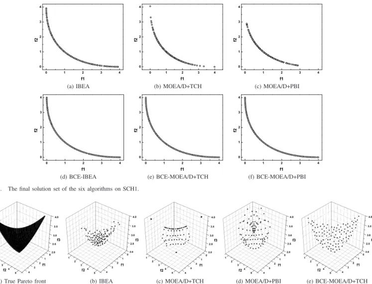
Fig. 4 plots the final solutions of the six algorithms in a single run on SCH1. This particular run, along with others for visual demonstration in the paper, is associated with the result which is the closest to the mean IGD value. SCH1 has

a convex Pareto optimal curve in the rangef1, f2∈[0,4]. As

shown, IBEA and MOEA/D+TCH struggle to maintain the uniformity of the solutions, especially around the edges of the true Pareto front. MOEA/D+PBI fails to find boundary points of the true Pareto front, with their solutions concentrating in

the range[0,3]. On the other hand, the three BCE algorithms

perform well. Their performance appears similar and all of their solutions are uniformly distributed along the whole true Pareto front. This happens mainly due to the population maintenance operation in BCE, which can effectively eliminate poorly distributed solutions in the evolutionary process. In the rest of the paper, for brevity, we only plot the solutions of one of the BCE algorithms if they perform visually similarly.

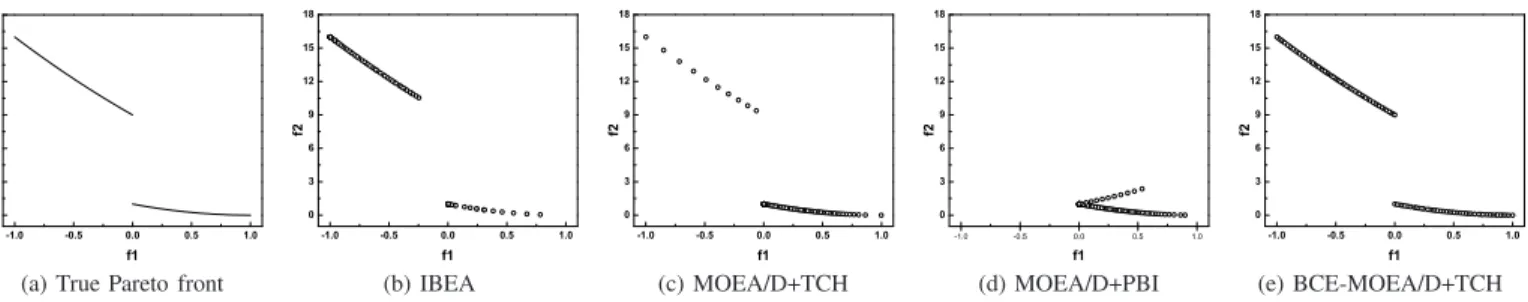
In addition, Fig. 5 shows the final solutions on VNT1.

Clearly, for this 3-objective problem, only the BCE algorithms have good diversity. The solutions obtained by IBEA are solely located in the middle of the true Pareto front. The solutions of the two MOEA/D algorithms, which correspond to uniformly distributed weight vectors, exhibit a specific structure but do not have a good distribution over the desired front.

B. Test Problems with a Concave True Pareto Front

In this category, we consider 13 problems from the ZDT, WFG, and DTLZ problem suites. As can be seen from Tables III and IV, the three BCE algorithms generally perform better than their competitors. Specifically, IBEA, BCE-MOEA/D+TCH, and BCE-MOEA/D+PBI obtain a better IGD value in 12, 8, and 9 out of the 13 test instances, respec-tively. For HV, IBEA, MOEA/D+TCH, and BCE-MOEA/D+PBI outperform their corresponding non-Pareto al-gorithms in 12, 9, and 9 out of the 13 instances, respectively. In fact, for some MOPs (such as DTLZ2), some non-Pareto algorithms already work quite well. In this case, the exploration operation in the PC evolution of BCE can hardly further improve individuals’ performance, but can

(11)

0 1 2 3 4 0 1 2 3 4 f 2 f1 0 1 2 3 4 0 1 2 3 4 f 2 f1 0 1 2 3 4 0 1 2 3 4 f 2 f1

(a) IBEA (b) MOEA/D+TCH (c) MOEA/D+PBI

0 1 2 3 4 0 1 2 3 4 f 2 f1 0 1 2 3 4 0 1 2 3 4 f 2 f1 0 1 2 3 4 0 1 2 3 4 f 2 f1

(d) BCE-IBEA (e) BCE-MOEA/D+TCH (f) BCE-MOEA/D+PBI

Fig. 4. The final solution set of the six algorithms on SCH1.

(a) True Pareto front (b) IBEA (c) MOEA/D+TCH (d) MOEA/D+PBI (e) BCE-MOEA/D+TCH

Fig. 5. True Pareto front and the final solution set on VNT1, where the solutions of the three BCE algorithms have similar distribution.

(a) IBEA (b) MOEA/D+TCH (c) MOEA/D+PBI (d) BCE-MOEA/D+TCH

Fig. 6. The final solution set on DTLZ2, where the solutions of the three BCE algorithms have similar distribution.

lead to the decrease of the computational resources (i.e., function evaluations) occupied by the NPC evolution. Fig. 6 gives the final solutions obtained by IBEA, MOEA/D+TCH, MOEA/D+PBI, and BCE-MOEA/D+TCH on DTLZ2. Clearly, for this problem, IBEA is unable to maintain uniformity of the solutions but MOEA/D+TCH and MOEA/D+PBI have a set of excellently distributed solutions over the true Pareto front. This is consistent with the result in Table III, where IBEA performs worse than BCE-IBEA but the two MOEA/D algorithms perform better than their competitors.

As to the statistical results, it can be observed from the tables that the difference between the paired algorithms is significant for most of the test instances. Specifically, the pro-portion of the test instances where the three BCE algorithms BCE-IBEA, BCE-MOEA/D+TCH and BCE-MOEA/D+PBI outperform their competitors with statistical significance is 11/13, 6/13 and 9/13 for IGD and 9/13, 9/13 and 9/13 for HV, respectively. Conversely, the proportion of the instances where the three non-Pareto algorithms IBEA, MOEA/D+TCH and MOEA/D+PBI are superior with statistical significance is

(12)

0.0 0.5 1.0 1.5 2.0 0 1 2 3 4 f 2 f1 MOEA/D+PBI Pareto front 0.0 0.5 1.0 1.5 2.0 0 1 2 3 4 f1 f 2 BCE-MOEA/D+PBI Pareto front

(a) MOEA/D+PBI (b) BCE-MOEA/D+PBI

Fig. 7. The final solution set obtained by MOEA/D+PBI and

BCE-MOEA/D+PBI on WFG3. 0.0 0.5 1.0 1.5 2.0 2.5 0.0 0.5 1.0 1.5 2.0 2.5 3.0 3.5 4.0 4.5 f 2 f1 MOEA/D+PBI BCE-MOEA/D+PBI Pareto front 0.0 0.5 1.0 1.5 2.0 2.5 0.0 0.5 1.0 1.5 2.0 2.5 3.0 3.5 4.0 4.5 MOEA/D+PBI BCE-MOEA/D+PBI Pareto front f 2 f1

(a) All the individuals produced (b) Population at the 1,000 evaluations

Fig. 8. Results of MOEA/D+PBI and BCE-MOEA/D+PBI during initial

1,000 function evaluations on WFG3: (a) All the individuals produced during the 1,000 evaluations; (b) Evolutionary population at the 1,000 evaluations.

0/13, 4/13 and 3/13 for IGD and 1/13, 4/13 and 1/13 for HV, respectively.

C. Test Problems with a Linear True Pareto Front

Non-Pareto EMO algorithms in general work well on this kind of problems as their NPC is not likely to prefer specific areas of a plane true Pareto front. Despite that, the proposed approach is still competitive, as can be seen from the results on test problems WFG3 and DTLZ1 in Tables III and IV. For WFG3, the three BCE algorithms all outperform their competi-tors. For a visual comparison, Fig. 7 plots the final solutions of MOEA/D+PBI and BCE-MOEA/D+PBI as well as the problem’s true Pareto front. As shown, BCE-MOEA/D+PBI has a better performance than MOEA/D+PBI in terms of both diversity and convergence. This observation is interesting because it is commonly believed that the solutions guided by an NPC have a better convergence than those by the PC. One important reason for this occurrence is that the exploration around the nondominated solutions in BCE can effectively drive the population evolving towards the true Pareto front, especially at the initial stage of evolution.

To take a closer look, Fig. 8 gives the results of MOEA/D+PBI and BCE-MOEA/D+PBI during the initial 1,000 function evaluations, where Fig. 8(a) plots all 1,000 individuals produced by the two algorithms and Fig. 8(b) plots their evolutionary population at the 1,000 evaluations. As can be seen from Fig. 8(a), there exist some individuals of BCE-MOEA/D+PBI apparently closer to the optimal front. This is the result of effective exploration of the nondominated indi-viduals (i.e., the PC population) in BCE. These nondominated

individuals, whose number is smaller than the population ca-pacity at that time, can represent the best individuals found so far, as seen from the comparison between Figs. 8(a) and (b). The test function DTLZ1 has a huge number of local

opti-mal fronts (115₋₁

). For this problem, BCE-IBEA outperforms IBEA, but BCE-MOEA/D+TCH and BCE-MOEA/D+PBI per-form worse than the two MOEA/D algorithms. In Section V-C, we will provide a detailed explanation for why BCE may be outperformed by some non-Pareto algorithms on such MOPs with a number of local optima.

D. Test Problems with a Mixed True Pareto Front

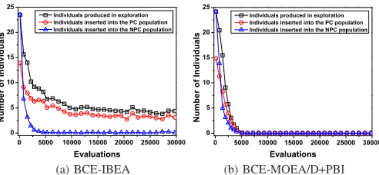
The results of three of this kind of problems, WFG1, VNT2 and VNT3, are shown in Tables III and IV, where the BCE algorithms significantly outperform their competitors. They are superior with statistical significance in 8 out of all the 9 comparisons for both IGD and HV indicators. For a visual observation, Fig. 9 plots the final solutions ob-tained by IBEA, MOEA/D+TCH, MOEA/D+PBI, and BCE-MOEA/D+TCH on VNT3. Clearly, only BCE-BCE-MOEA/D+TCH has well-distributed solutions over the whole true Pareto front. The solutions obtained by the three non-Pareto algorithms concentrate mainly in the middle segment and fail to extend to the left part of the optimal front.

E. Test Problems with a Discontinuous True Pareto Front

As can be seen from the two tables, for MOPs with a discontinuous true Pareto front, the proposed approaches have a clear advantage over the non-Pareto algorithms. The three BCE algorithms significantly outperform their competitors for all the instances, and on most of these instances they even have an order of magnitude smaller IGD values.

In fact, non-Pareto algorithms commonly struggle to main-tain the diversity of solutions on this kind of MOPs. This happens mainly due to the fact that the imaginary parts of the discontinuous true Pareto front largely affect the accuracy of the fitness estimation based on an NPC. For example, in MOEA/D, the breakpoints of the discontinuous true Pareto front may correspond to the optimal solution of multiple scalar subproblems [54]. This is likely to cause the failure of uniformity maintenance of solutions, further leading to the search of the algorithm only on some specific regions of the objective space. Fig. 10 plots the final solutions ob-tained by IBEA, MOEA/D+TCH, MOEA/D+PBI, and BCE-MOEA/D+TCH on SCH2. It can be observed that IBEA and MOEA/D+TCH are unable to maintain the uniformity of solu-tions, and MOEA/D+PBI fails to find the upper part of the true Pareto front. Note that there exist some dominated solutions in the set of solutions obtained by MOEA/D+PBI. This is because a dominated solution may have a closer distance than a nondominated one to the corresponding reference point in MOEA/D+PBI, as pointed out in [16].

F. Test Problems with a Complex PS

In this section, we consider the UF problem suite from the CEC2009 competition [70]. These MOPs involve a strong linkage in variables among the Pareto optimal solutions,