Software Requirements Classification Using Word Embeddings and Convolutional Neural Networks

SOFTWARE REQUIREMENTS CLASSIFICATION USING WORD EMBEDDINGS AND CONVOLUTIONAL NEURAL NETWORKS

A Thesis presented to

the Faculty of California Polytechnic State University, San Luis Obispo

In Partial Fulfillment

of the Requirements for the Degree Master of Science in Computer Science

by Vivian Fong

c 2018 Vivian Fong

COMMITTEE MEMBERSHIP

TITLE: Software Requirements Classification Us-ing Word EmbeddUs-ings and Convolutional Neural Networks

AUTHOR: Vivian Fong

DATE SUBMITTED: June 2018

COMMITTEE CHAIR: Alexander Dekhtyar, Ph.D. Professor of Computer Science

COMMITTEE MEMBER: David Janzen, Ph.D.

Professor of Computer Science

COMMITTEE MEMBER: Foaad Khosmood, Ph.D. Professor of Computer Science

ABSTRACT

Software Requirements Classification Using Word Embeddings and Convolutional Neural Networks

Vivian Fong

Software requirements classification, the practice of categorizing requirements by their type or purpose, can improve organization and transparency in the requirements engineering process and thus promote requirement fulfillment and software project completion. Requirements classification automation is a prominent area of research as automation can alleviate the tediousness of manual labeling and loosen its necessity for domain-expertise.

This thesis explores the application of deep learning techniques on software re-quirements classification, specifically the use of word embeddings for document rep-resentation when training a convolutional neural network (CNN). As past research endeavors mainly utilize information retrieval and traditional machine learning tech-niques, we entertain the potential of deep learning on this particular task. With the support of learning libraries such as TensorFlow and Scikit-Learn and word embed-ding models such as word2vec and fastText, we build a Python system that trains and validates configurations of Na¨ıve Bayes and CNN requirements classifiers. Apply-ing our system to a suite of experiments on two well-studied requirements datasets, we recreate or establish the Na¨ıve Bayes baselines and evaluate the impact of CNNs equipped with word embeddings trained from scratch versus word embeddings pre-trained on Big Data.

ACKNOWLEDGMENTS

Thanks to:

• Professor Alex Dekhtyar for guiding me through my academic endeavors and sparking my interest in machine learning.

• Thesis-depression buddies Tram, Irene, and Mike. Misery loves company. • Thesis veterans Nupur, Katie, and Andrew for their counseling and

encourage-ment.

• Shelby and the Johannesens for graciously letting me stay with them during my last visits to SLO.

• Lexus, Jacob, Esha, and Gary for retaining some remnants of my social life. • Laura, JoJo, and David for being my backbone and personal cheer squad. • Mom and Dad for forever loving and supporting me, feeding me delicious

home-cooked meals and treating me like the spoiled princess I am.

• Every coffee shop I step foot in, laptop in hand, during my entire graduate career.

TABLE OF CONTENTS Page LIST OF TABLES . . . ix LIST OF FIGURES . . . xi CHAPTER 1 Introduction . . . 1 2 Background . . . 5 2.1 Requirements Specifications . . . 5 2.1.1 Requirements Classification . . . 5 2.2 Machine Learning . . . 7 2.2.1 Na¨ıve Bayes . . . 9 2.2.2 Perceptrons . . . 10

2.2.3 Support Vector Machines . . . 10

2.3 Deep Learning . . . 12

2.3.1 History . . . 12

2.3.2 Neural Networks . . . 13

2.3.3 Convolutional Neural Networks . . . 16

2.4 Natural Language Processing . . . 20

2.4.1 Text Preprocessing . . . 20 2.4.2 Vector Representations . . . 21 2.5 Model Validation . . . 25 2.5.1 Cross-Validation . . . 25 2.5.2 Overfitting . . . 25 2.6 Performance Metrics . . . 26 2.6.1 Confusion Matrix . . . 26 2.6.2 Accuracy . . . 27

2.6.3 Recall, Precision, and Fβ-score . . . 27

2.6.4 Cross-Entropy Loss . . . 28

2.7 Tools . . . 28

2.7.2 Scikit-Learn . . . 29

2.7.3 Gensim . . . 29

2.7.4 TensorFlow . . . 29

2.8 Datasets . . . 30

2.8.1 Security Requirements (SecReq) . . . 30

2.8.2 Quality Attributes (NFR) . . . 32

2.9 Prior Work . . . 34

2.9.1 Classifying Security Requirements . . . 34

2.9.2 Classifying Quality Attributes . . . 35

3 Design and Implementation . . . 39

3.1 Run Configurations . . . 41

3.2 Data Loading and Preprocessing . . . 42

3.2.1 Raw Data Formats . . . 42

3.2.2 Classifier Input Format . . . 44

3.2.3 Training and Test Set Division . . . 45

3.2.4 Pre-trained Embedding Model Loading . . . 45

3.3 Classifier Training . . . 46

3.3.1 CNN . . . 46

3.3.2 Na¨ıve Bayes . . . 50

3.3.3 Testing and Result Compilation . . . 50

3.4 Exportation . . . 51

4 Experiments and Results . . . 52

4.1 Experiment 1: Na¨ıve Bayes Baselines . . . 54

4.1.1 SecReq-SE . . . 54

4.1.2 NFR-NF . . . 55

4.1.3 NFR-Types . . . 55

4.1.4 NFR-SE . . . 56

4.2 Experiment 2: Optimal CNN Models for Binary Classification . . . . 56

4.2.1 SecReq-SE . . . 59

4.2.2 NFR-NF . . . 60

4.2.3 NFR-SE . . . 60

4.3 Experiment 3: Optimal CNN Models for Multi-label Classification . . 62

4.3.1 NFR-Types: Multi-label . . . 63

4.3.2 NFR-Types: Binary CNNs . . . 64

4.3.3 Discussion . . . 64

4.4 Experiment 4: Epoch Convergence . . . 65

4.4.1 SecReq-SE . . . 65

4.4.2 NFR-NF . . . 68

4.4.3 Discussion . . . 69

4.5 Experiment 5: Cross-Dataset Security Requirements Classification . . 69

4.5.1 Train on SecReq-SE, Validate on NFR-SE . . . 70

4.5.2 Train on NFR-SE, Validate on SecReq-SE . . . 71

4.5.3 Hybrid Security Dataset . . . 72

4.5.4 Discussion . . . 73 5 Related Work . . . 74 5.1 Preprocessing Strategies . . . 74 5.1.1 Comparison . . . 75 5.2 Sampling Strategies . . . 76 5.2.1 Comparison . . . 77

5.3 Domain-Independent Model and One-Class SVMs . . . 78

5.3.1 Comparison . . . 79

5.4 Topic Modeling, Clustering, and Binarized Na¨ıve Bayes . . . 80

6 Conclusions and Future Work . . . 81

6.1 Future Work . . . 84 6.1.1 One-vs.-All Classification . . . 84 6.1.2 CNN Optimization . . . 84 6.1.3 Word Embeddings . . . 85 6.1.4 FastText . . . 86 BIBLIOGRAPHY . . . 87 APPENDICES A TF-IDF Experiments . . . 93

LIST OF TABLES

Table Page

2.1 Examples of functional and non-functional requirements from the

NFR dataset. . . 6

2.2 Confusion matrix legend. . . 26

2.3 SecReq dataset, broken down by SRS [25]. . . 30

2.4 Examples of security-related and not security-related requirements from SecReq. . . 31

2.5 NFR dataset, broken down by project and requirements type [14]. . 32

2.6 Examples of requirements of different types from NFR. . . 33

2.7 SecReq Na¨ıve Bayes classification experiments by Knauss et al. [26]. 35 2.8 Results from using top-15 terms at classification with threshold value of 0.04, by Cleland-Huang et al. [14]. . . 37

3.1 Run configuration options. . . 42

3.2 WordEmbeddingCNNhyperparameters. . . 47

3.3 Embedding matrix example (d= 5, n= 7, N = 10). . . 48

4.1 SecReq and NFR primary classification problems. . . 52

4.2 Na¨ıve Bayes results for SecReq-SE binary classification. . . 54

4.3 Na¨ıve Bayes (with CountVectorizer) results for NFR-NF binary classification. . . 55

4.4 Na¨ıve Bayes (withCountVectorizer) results for NFR-Types multi-label classification and individual NFR multi-label binary classification. . 56

4.5 SecReq-SE: Optimal CNN model results, trained with 140 epochs. . 59

4.6 SecReq-SE: Loss and F1-score from optimal CNN models applied to each word embedding type. . . 59

4.7 NFR-NF: Optimal CNN model results, trained with 140 epochs. . . 60

4.8 NFR-NF: Loss and F1-score from optimal CNN models applied to each word embedding type. . . 60

4.9 NFR-SE: Optimal CNN model results, trained with 140 epochs. . . 61

4.10 NFR-SE: Loss and F1-score from optimal CNN models applied to each word embedding type. . . 61

4.11 NFR-Types: Optimal multi-label CNN model results, trained with 140 epochs. . . 63 4.12 NFR-Types: Individual binary CNN results, trained with 140 epochs. 64 4.13 Results from NB and CNN classifiers trained on SecReq-SE, validated

on NFR-SE using 10-fold cross-validation. . . 70 4.14 Results from NB and CNN classifiers trained on SecReq-SE, validated

on NFR-SE, without cross-validation. . . 70 4.15 Results from NB and CNN classifiers trained on NFR-SE, validated

on SecReq, using 10-fold cross-validation. . . 71 4.16 Results from NB and CNN classifiers trained on NFR-SE, validated

on SecReq, without cross-validation. . . 72 4.17 Results from NB and CNN classifiers trained and validated on

secu-rity hybrid dataset, using 10-fold cross validation. . . 73 5.1 NFR-NF binary classification results from Abad et al. [9] compared

to our CNN word embedding approaches. . . 76 5.2 NFR-US and NFR-PE binary classification results from Kurtanovi´c

et al. [29] compared to our CNN word embedding approaches. . . . 78 5.3 Comparison of most effective security requirements classifiers on

sin-gle domain evaluations between Knauss et al. [26], Munaiah et al. [37], and our CNN word embedding approaches. . . 79 6.1 Summary of NB baseline and CNN performance for binary

classifi-cation problems, trained with 140 epochs and run with 10-fold cross-validation. . . 82 6.2 Summary of NB baseline and CNNF1-scores for NFR-Types

multi-label classification, trained with 140 epochs and run with 10-fold cross-validation. . . 82 6.3 Summary of NB baseline and CNNT P count for NFR-Types

multi-label classification, trained with 140 epochs and run with 10-fold cross-validation. . . 83 A.1 Na¨ıve Bayes (with TfidfVectorizer) results for SecReq-SE binary

classification. . . 93 A.2 Na¨ıve Bayes (with TfidfVectorizer) results for NFR-NF binary

classification. . . 93 A.3 Na¨ıve Bayes (withTfidfVectorizer) results for NFR-Types

LIST OF FIGURES

Figure Page

2.1 Example of a support vector machine for the linearly non-separable

case. . . 11

2.2 Example of a neural network with three hidden layers. . . 14

2.3 CNN architecture for image classification (adapted from LeCun et al. [31]). . . 17

2.4 CNN architecture for sentence classification (adapted from Zhang et al. [45]). . . 19

2.5 Skip-gram model (adapted from Mikolov et al. [34]). . . 23

2.6 Recall and precision results from one-vs.-all multi-label classification of NFR types from Casomayor et al. [11]. . . 38

3.1 System design activity diagram. . . 40

3.2 Examples of SecReq raw data format. . . 43

3.3 Example of NFR raw data format. . . 43

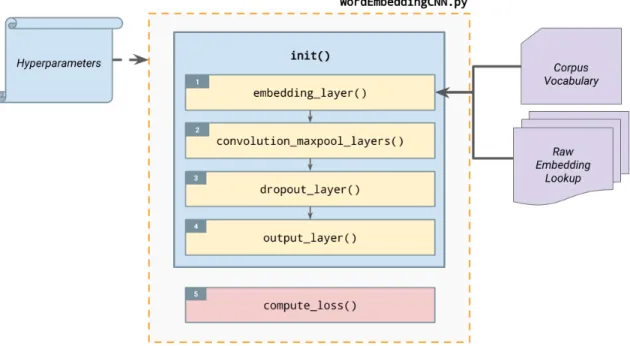
3.4 Illustration of WordEmbeddingCNN layer initialization. . . 46

4.1 # of Epochs vs. Performance for SecReq-SE optimal CNN. . . 66

Chapter 1 INTRODUCTION

Requirements engineering (RE) describes the process of discovering, documenting, and maintaining requirements during the software development life cycle [43]. Re-quirements outline the business needs and use cases that establish the necessity of a product, as well as overall system performance criteria. Whether it be for a school assignment or industry development, the modeling and fulfillment of requirements is crucial to measuring a product’s completion and a team’s success. Design and imple-mentation decisions should all directly correlate with requirements established within the project.

Software requirements can be of different types, encapsulating criteria within a specific area of interest in the software product. For example, requirements can be classified as functional (explicit features, or functions, of the product) or non-functional (implicit quality criteria for the product), which can be further drilled into more specific categories. Furthermore, requirements may serve different pur-poses, from highlighting security vulnerabilities to measuring scalability necessities to assessing general look-and-feel [4, 14]. Identifying all requirements of a specific type (i.e., security-related) allows engineers and other participants of the software develop-ment cycle to hone in on particular non-functional concerns for the system and assess project completeness, ultimately promoting awareness of requirements that are often overlooked. Software specialists can immediately locate which requirements interest them without needed to peruse through the entire SRS (e.g., the UX designer is likely interested in look-and-feel requirements). However, the manual task of labeling what category a requirement falls under is tedious. On top of that, manual requirements labeling requires domain-expertise, which can be limited and expensive, highlighting

the need to explore automated methods.

Automated requirements labeling can be defined as a machine learning classifi-cation problem. Machine learning is a sub-field within artificial intelligence that en-compasses a type of algorithm that discovers, or learns, patterns from existing data, detecting trends to help make predictions on new data [36]. Classification is the ma-chine learning task of identifying which category out of a set of categories an item belongs to [19]; it requires a set of pre-labeled data to learn from, using that knowledge to predict the labels for unseen data. Previous automated requirements classification research primarily investigate traditional learning and vectorization methods such as Na¨ıve Bayes and TF-IDF.

In this thesis, we aim to study the impact of deep learning, a subdivision within machine learning, on the classification of software requirements. Deep learning tech-niques, characterized by multi-layer graphs of data transformation, are booming in popularity with their breakthroughs in machine translation, image and voice recog-nition, and other fields within technology. In recent years, deep learning has helped develop a way to transform text into a medium that computers can consume and extract semantic information from, making advancements towards replicating the hu-man ability to process language. At their core, requirements specifications are plain text documents that can be processed like natural language. They are commonly very short in length and written in formal language with domain-specific diction. In addition, requirements specifications contain a relatively small volume of samples. These characteristics foster an unconventional environment for deep learning as such methods are often applied on extremely large datasets of feature-rich samples.

We investigate two specific aspects of deep learning: (1) convolutional neurals networks to train a classifier in performing requirements classification, and (2) word embeddings to represent our requirements documents. A convolutional neural

net-work (CNN) is a deep neural netnet-work designed to learn from a grid-like topology in the input data [19]. Traditionally, CNNs are used to tackle image recognition tasks, but its efficacy in text classification has been recently proven [23]. Word embeddings are rich vector representations of words that claim to capture syntactic and semantic relationships between words, resultant from training neural networks on very large corpora (“Big Data”) [35, 34]. This leads us to pose our primary research questions: 1. RQ1: Can deep learning models such as CNNs offer competitive performance

on software requirements classification?

2. RQ2: Can leveraging the power of Big Data when vectorizing our documents with pre-trained word embeddings boost CNN performance on software require-ments classification?

Our paper to the 25th International IEEE Requirements Engineering Conference titled “RE Data Challenge: Requirements Identification with Word2Vec and Tensor-Flow” [17] initiates our research with a replication of prior work baselines in addition to a pilot assessment of word2vec word embeddings and TensorFlow CNNs on two binary requirements classification problems. Since that paper, we dive deeper into the study to assemble the following list of contributions:

1. Recreation or establishment of Na¨ıve Bayes baselines.

2. Feasibility assessment of CNNs on binary and multi-label requirements classifi-cation.

3. Comparison of three word embedding methods in assisting requirements docu-ment representation when training CNNs.

The rest of this document is organized as follows: Chapter 2 dives into the background in software requirements engineering, machine learning methodology and tools, as well as the datasets we utilize and some prior work. Chapter 3 details our system design, and Chapter 4 outlines our experiments and discusses their results. Chapter 5 briefly discusses the current related work active in the field. Lastly, Chapter 6 summarizes our conclusions and future work.

Chapter 2 BACKGROUND

2.1 Requirements Specifications

Upon the launch of a product idea, product managers in software teams need to understand the needs of their potential customers and users, a process called require-ments elicitation. Depending on the development style adopted by the team, the requirements elicitation process may take a long time to complete. The artifacts pro-duced during this process are software requirements specifications (SRS), documents that list and detail each user or system requirement that needs to be satisfied for the product to be complete.

Various types of requirements are considered during requirements elicitation. Func-tional requirements (FR) can define specific behaviors, features, and use cases of the product. FRs can be broken down into high-level requirements (HLR) and low-level requirements (LLR). HLRs can be abstract statements defining an overall feature needed, and LLRs are more detailed descriptions of what the product needs in order to realize the HLR. Non-functional requirements (NFR), on the other hand, assess system properties and constraints such as performance, scalability, and security [43]. In short, FRs describe what the system should do and NFRs describe how the sys-tem should perform it [18]. Table 2.1 showcases some examples of functional and non-functional requirements.

2.1.1 Requirements Classification

Requirements elicitation, SRS documentation, and maintenance all make up a process called requirements engineering (RE) [43]. An area of research within requirements

Table 2.1: Examples of functional and non-functional requirements from the NFR dataset.

Requirement Type Requirements Text

Functional “The system will notify affected parties when changes occur affecting classes including but not limited to class cancellations class section detail changes and changes to class offerings for a given quarter.”

Performance “Any interface between a user and the automated system shall have a maximum response time of 5 seconds unless noted by an exception below.”

Scalability “The product shall be capable of handling up to 1000 concurrent requests. This number will increase to 2000 by Release 2. The concurrency capacity must be able to handle peak scheduling times such as early morning and late afternoon hours.” Security “User access should be limited to the permissions granted to their role(s) Each level

in the PCG hierarchy will be assigned a role and users will be assigned to these roles. Access to functionality within RFS system is dependent on the privileges/permission assigned to the role.”

engineering is requirements classification.

Requirements classification (or requirements identification) is the task of identi-fying requirements as belonging to a specific category, thus highlighting their role in the project. Two examples of classification tasks are (1) distinguishing between func-tional and non-funcfunc-tional requirements, and (2) determining whether a non-funcfunc-tional requirement is related to concerns such as security, performance, reliability, etc [14].

NFRs are important because they pinpoint areas that affect the health and well-being of the system as a whole rather than just a single feature in a module. Fulfilling them requires not only careful design decisions in the beginning, but also continuous effort throughout the entire software development process. Unfortunately, as Kur-tanovi´c et al. concludes [29], NFRs are often identified later in the software process [12, 29] and are vaguely described and poorly managed [18], causing engineers to ne-glect their importance [11]. Classifying requirements can help promote transparency and organization within the SRS and stimulate awareness toward crucial system

con-cerns that should be as much of a priority to engineers as feature development. However, manually classifying requirements calls for engineers who have exper-tise in the respective areas (i.e., proper identification of security requirements calls for security knowledge). This resource barrier can discourage project managers and engineers from properly assessing NFRs throughout the development process, leav-ing neglected or unidentified issues in the back seat and thus amplifyleav-ing the risk for defects, performance inadequacies, and technical debt. Automating this task can al-leviate the need for domain-experts, which in turn can promote the practice within the software community. In order to automate requirements classification, we must explore machine learning methodologies.

2.2 Machine Learning

Machine learning is a sub-field within AI that studies the making of predictions on data by learning from the characteristics of past samples [36]. Machine learning is a form of applied statistics that utilizes computers to estimate extremely complex functions [19], making it a powerful mechanism for solving abstract problems that are too difficult for humans to specify explicit algorithms for [36].

Machine learning algorithms can be divided into two categories: supervised and unsupervised learning. Supervised learning is the category of learning algorithms that builds a model by training on data that have been annotated with labels [19]. Having pre-labeled training data provides the model information as to how many classes exist within the data, allowing the model to focus on analyzing the features that distinguish these particular classes instead of formulating groups from scratch. Oftentimes, the requisite for labeled data poses a hurtle as most data in this world are untagged and manual tagging is often impractical. In contrast, unsupervised learning algorithms train on unlabeled data [19]. The advantage of unsupervised methods is

their disregard for explicit labeling. In the process, the model generates predictions of the possible distinguishing groups within the data.

Machine learning can be utilized to tackle a variety of problem areas, including regression, classification, and anomaly detection [19]. The work of this thesis focuses on supervised learning approaches to classification problems.

Classification

Classification is the task of determining which category, or class, out of k categories an input belongs to [19]. More formally, with an input vector x, a classification algorithm needs to formulate a function f : IRn → {1, . . . , k} so that y = f(x), outputting the predicted class y [19].

A classic example of binary classification is the image recognition task of distin-guishing whether a photo of a fluffy animal is one of a cat or dog. The input can be represented as a matrix of numerical pixel values x, and the output can be a one-hot vector y signaling which class the image is predicted to belong to. The example becomes a multi-label classification problem if we add more animals into the list of possible animal categories.

Numerous different types of learners can perform the task of classification, also known as classifiers. In the following subsections, we discuss Na¨ıve Bayes, percep-trons, and support vector machines. Rather than perform a deep dive into the math-ematics or algorithms, the purpose of these sections is to provide a brief introduction to the nature and construction of these classifiers.

2.2.1 Na¨ıve Bayes

The Bayesian learner, also known as theNa¨ıve Bayes (NB) classifier, is a straightfor-ward probabilistic approach [36]. Despite its simplicity, Na¨ıve Bayes is very practical and its performance can sometimes rival more sophisticated methods [36]. Conse-quently, NB is often a common first choice when tackling text classification tasks.

As this thesis involves textual requirements, we will explain NB in terms of docu-ment analysis. Given categoriesC={c1, . . . , c|C|}and documentsD={d¯1, . . . ,d¯|D|},

the probability P that the document ¯dj belongs to category ci is computed in Bayes

Theorem [41, 36]:

P(ci |d¯j) =

P(ci)P( ¯dj |ci)

P( ¯dj)

(2.1) where document ¯dj = hw1j, . . . , w|T|ji is represented by a vector of weights for each

term in the vocabulary set T from all documentsD. The topic of vector representa-tions is further elaborated in Section 2.4.2.

P( ¯dj) is the probability that a random document in the corpus is represented by

vector ¯dj, and P(ci) is the probability that a random document in the corpus is of

category ci [36]. Because the number of possible variations for ¯dj is too high,

com-putingP(ci |d¯j) can be impossible. To alleviate this bottleneck, an assumption that

“any two coordinates of the document vector are, when viewed as random variables, statistically independent of each other” is made [41]. This independence assumption is what characterizes this method as a na¨ıve approach. Equation 2.2 is the formula for the independence assumption [41, 36]:

P( ¯dj |ci) =

|T|

Y

k=1

2.2.2 Perceptrons

A perceptron is a simple linear binary classifier that determines a function that can bisect linearly separable data into two classes in d-dimensional space [32].

Let X = {¯x1, . . . ,x¯n} represent the set of data points where each sample ¯xi is

represented by a d-dimensional vector langlea1, . . . , adi. With C ={+1,−1} as the

set category labels, let Y = {y1, . . . , yn} where yi ∈ C so that yi is the true class of

the input ¯xi. Given a vector ofweights w= hw1, . . . , wdi and threshold value θ, the

perceptron function f(¯x) = w·x¯= d X j=1 wj·aj (2.3)

determines the class of input ¯x with the following decision procedure:

class(¯x) =        +1 iff(¯x)> θ −1 iff(¯x)< θ (2.4)

The f(¯x) = θ case is always counted as a misclassification [32].

Training a perceptron requires iterative fine-tuning of weight vector w until ei-ther (1) the function f(¯x) either correctly classifies all ¯x ∈ X, or (2) the error rate converges and stops decreasing [32]. Essentially, with each iteration of the training algorithm, the perceptron function tilts and adjusts in the d-dimensional space until it can successfully separate the two classes. Perceptrons are limited to a single linear hyperplane, rendering them useless in cases with non-linear or ambiguous separation boundaries.

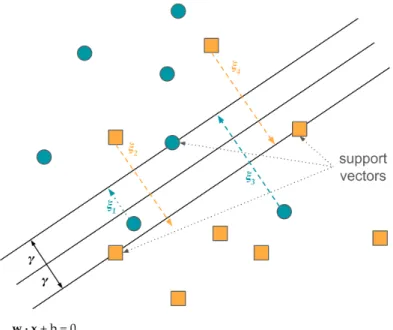
2.2.3 Support Vector Machines

Asupport vector machine (SVM) is essentially an improved perceptron that can clas-sify non-linearly separable data [32]. A SVM determines the optimal hyperplane that

Figure 2.1: Example of a support vector machine for the linearly non-separable case.

divides the two classes of data and maximizes the distance between the hyperplane and the closest data samples [32, 44, 41]. Adopting the same variable definitions as Section 2.2.2, the function for the hyperplane is defined as follows [44]:

h(¯x) =w·x¯+b= (

d

X

j=1

wj ·aj) +b= 0 (2.5)

where b is a constant scalar value called the bias which can be treated the same as the negative of the threshold θ in our discussion of perceptrons [32, 44].

The data points with the shortest distance γ (also referred to as the margin) to the hyperplane are known as support vectors. The goal of the SVM is to determine the weight vector w and bias b that maximize γ such that for all i = 1, . . . , n, the following condition is fulfilled [32]:

yi ·(w·x¯i+b)≥γ (2.6)

of one class that on the wrong side of the hyperplane. To address this, Equation 2.6 can be revised by introducing slack variables ξi [32]:

yi·(w·x¯i+b)≥1−ξi, ξi >0 (2.7)

Penalties can be added (with the hinge loss function) to account for data points that might be on the wrong side of the hyperplane [32]. SVMs can also use kernal tricks to build non-linear separating curves.

2.3 Deep Learning

Deep learning is a subcategory of machine learning that solves a complex problem by learning from a hierarchy of smaller, simpler representations, building a deep graph of concepts with many layers [19].

2.3.1 History

Deep learning has a long train of history dating back to the 1940s, adopting several aliases and riding waves of different philosophies throughout the decades. Although the methodology is a current hot topic, deep learning has remained dormant and unpopular for most of its history [19].

The first wave was introduced with the study of cybernetics in biological learning and implementations of the perceptron in the 1940s–1960s. The second wave came between 1980–1995 with the concept of backpropagation and neural network training. Finally, the third and current wave arrived in 2006, adopting the buzzword deep learning that we know and love today. Today’s appreciation for deep learning is thanks to modern day computing infrastructure and growing data availability [19, 31], allowing researchers and industry to utilize the science with their massive volumes of data, contributing significant advancements in AI.

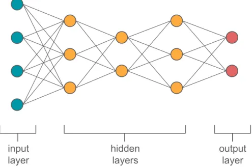
2.3.2 Neural Networks

The fundamental example of a deep learning model is the deep feedforward neural network, a concept loosely inspired by the shape and nature of neural connectivity within the brain. A neural network estimates a mathematical function f∗ mapping some input ¯x to some class labely, composed of a web of simpler intermediate func-tions [19]. The model is also known as the multi-layer perceptron (MLP) as it can be seen as an “acyclic network of perceptrons”, with the output of some perceptrons used as the input to others [32]. Each individual perceptron in the network is known as a neuron, with the fundamental difference being the use of a non-linear activation function rather than a unit-step decision function. The following subsections describe the architecture and training of a neural network.

Architecture

In a feedforward neural network, the input ¯x flows through the network of functions to reach an output ˆy [19].

As shown in Figure 2.2, the initial layer to the network is the input layer, repre-senting the units of the input vector ¯x. The subsequent layers are known as hidden layers. If the neural network f(¯x) is composed of three chained functions such that f(¯x) = f3(f2(f1(x))), f1 is the first hidden layer of the network, f2 the second, and

f3 the third. These layers are “hidden” because the output of each function fi are

unknown to the input data. Finally, the last layer of a feedforward network is the output layer, which represents the class label ˆyconcluded by the classifier. The length of the chain determines the depth of the network (hence “deep” learning).

Each neuron in its layer works in parallel. A neuron receives a vector of inputs and weights from the previous layer to serve as an input to its activation function,

Figure 2.2: Example of a neural network with three hidden layers.

a non-linear sigmoid function g (i.e., σ(x), tanh(x), ReLU) that we choose when designing the model [19]. In other words, the output of a neuron is g(P

wixi), the

activation function applied on the sum of the scalar product between the weight and input vectors from the previous layer, which is then sent over to the next layer as an input.

In the case of SVMs and neural networks, we need to select a cost function that represents the error of the modelf(w, b) to optimize. Standard cost functions include sum-squared error and cross-entropy loss [19]. Cross-entropy loss is discussed in Section 2.6.4.

Gradient Descent

Gradient descent is a useful iterative approximation technique employed to train many types of machine learning models. It looks for the optimal value for multivariate functions, computing the gradient of the function and tuning the parameters with each learning step to approach a local optima [32].

Let η be the learning rate, or the fraction of the gradient we move w by in each round. During each iteration, each wj ∈ w gets adjusted by the following formula

[32]:

wj :=wj −η∇f(wj) (2.8)

It is evident that the learning rateηcan play a large role in how quickly or accurately gradient descent can perform; the weights might take too long to converge if η is too small, whereas if η is too large, the optimum can be missed. Optimization algo-rithms, such as Adam [24], have been developed to provide sophisticated strategies to optimizing the learning rate and the performance of gradient descent.

Training

The outline below describes the steps to training a neural network [19]:

1. Initialization. Initialize the weights w for each neuron in the hidden and output layers.

2. Learning Step. Each learning step is performed in two stages:

• Forward Propagation. On each step s, propagate a batch of input points Xs ⊆X through the network and compute the cost of the model with the

current weights.

• Back Propagation. Apply gradient descent on the current batch Xs from

the output layer through the hidden layers to adjust the weights of the neurons.

3. Termination. Terminate once either the cost converges or drops below a cer-tain threshold.

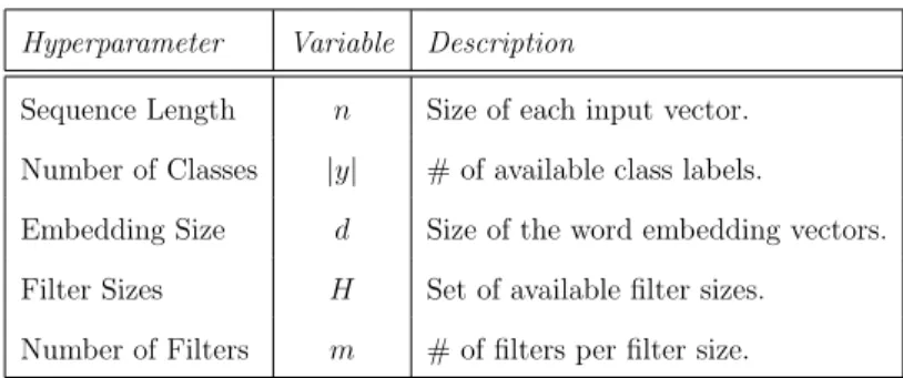
Hyperparameters

Hyperparameters are settings for the classifier that need to be determined before training [13, 19]. In the case of neural networks, the number of hidden layers and the number of neurons per layer , learning rate, and activation function are examples of hyperparameters that need to be set prior to training. The selection of hyperparam-eters can greatly affect the performance of the model, however finding the optimal combination of settings is proven to be an ongoing challenge in machine learning [13].

2.3.3 Convolutional Neural Networks

Theconvolutional neural network (CNN) is an evolution of the multi-layer perceptron that specializes in automatic feature extraction [42] from data that can be processed in a “grid-like topology” [19]. In other words, CNNs are designed to take advantage of the locality and order of the input elements when learning, making it compatible with tasks involving pattern recognition [17, 31]. The following subsection describes the general architecture of a CNN for image recognition, followed by a deeper discussion of a CNN model designed for sentence classification.

CNN Architecture

CNNs are composed of a stack of three types of layers: convolutional, pooling, and fully-connected layers [38, 19]. Figure 2.3 illustrates an example architecture for a CNN meant to classify handwritten digits from the MNIST dataset [31].

Input Layer. Just like with traditional neural networks, the input layer for a CNN takes in a vector of input values. In the case of the image processing, the input is a n×n matrix of pixel values representing the image. The input can also be expanded in dimensionality to encompass multiple channels of values per unit in the grid (e.g.,

Figure 2.3: CNN architecture for image classification (adapted from Le-Cun et al. [31]).

RGB values per pixel).

Convolutional Layer. In theconvolutional layer, afilter of sizeh×his used to slide across the input matrix, capturingn−h+ 1 regions of the input calledconvolutions. Each convolution acts as a neuron, computing the scalar product between its weights and regional input, followed by the activation function (namely rectified linear unit, or ReLU) [38], resulting in a single feature. The features from each convolution are aggregated into a feature map for each filter.

Pooling Layer. The pooling layer reduces the dimensionality of its input by a pro-cess called subsampling [38, 19]. An example of subsampling is max-pooling where the greatest value from the neural outputs from the convolutions from a particular region is taken and the rest are discarded.

Fully-Connected Layers. The fully-connected layers that follow perform the same operations as traditional neural networks — calculating scores to derive a prediction of which class the input belongs to [38, 31]. A softmax layer is often used as the final layer to a neural network, using the softmax function to normalize the output from

the final hidden layer into probability values for each output class [45, 23]. Dropout can also be applied to the softmax layer as a means of regularization — randomly “turning off” neurons in the network by randomly settings values in the weight vector to 0 in efforts to prevent overfitting [45]. The concept of overfitting is further discussed in Section 2.5.2.

Through a combination of convolutional and pooling layers, CNNs transform the complexity of the original input data, extracting the core patterns that distinguish one class from another from the training data.

One-Layer CNN for Sentence Classification

Although originally designed for image recognition [28], CNNs have also been proven to be effective textual contexts as well [15, 23]. We will discuss the one-layer CNN architecture Kim et al. has designed for sentence classification [23], illustrated in Figure 2.4.

Embedding Layer. We refer to the input layer in a sentence classification CNN as the embedding layer, as the input sentence is formulated as a two-dimensional embedding matrix built by concatenating together d-dimensional word vector repre-sentations for each of the n tokens in the sentence [23, 45]. Figure 2.4 showcases an example where the input sentence"This was a terrible disappointment!" is transformed into an embedding matrix with 5-dimensional word embeddings. Word embeddings are further discuss in Section 2.4.2.

Convolutional and Pooling Layers. The convolutional layer for a sentence classi-fication CNN uses filters of size h×d to build n−h+ 1 convolutions of the input, representingn-grams of sizehwithin the sentence [23, 45]. Ann-gram is a continuous sequence of ntokens in a sample of text. These n-grams are analogous to the regions

Figure 2.4: CNN architecture for sentence classification (adapted from Zhang et al. [45]).

of pixels in an image, hoping to capture location-based features within the input. Following the convolutional layer is a pooling layer where subsampling is per-formed to record the best outcome from each filter’s feature map. Max-pooling is often employed to capture the most important feature from each feature map [23, 45]. The selected outputs from each feature map are then concatenated into a single feature vector, which is then funneled into the remaining layers of the network.

Although we allude in the earlier discussion of image classification CNNs that the architecture can support a series of convolutional and pooling layers, Kim et al. designed their sentence classification CNN with a single convolutional and pooling layer [23]. The single convolutional layer can support a number of different filter sizes, thus capturing various forms ofn-grams. Figure 2.4 illustrates an example with two filter sizes 3×5 and 4×5 (h1 = 3, h2 = 4), representing 3-grams and 4-grams.

convolutions of size 3×5 and m·(n−h2 + 1) = 6 convolutions of size 4×5. The

results from each convolution aggregate into a feature map of shape (n−h+ 1)×1 for each filter.

Fully-Connected Layers. The remainder of the network is identical to the image processing CNN; the network needs to convert the feature vector from the pool-ing layer into class prediction scores (i.e., softmax layer with optional regularization methods).

2.4 Natural Language Processing

Natural language processing (NLP) studies the interpretation and generation of nat-ural language by computers [21].

2.4.1 Text Preprocessing

Text preprocessing, a pipeline of cleaning operations to transform the raw, free-form text into a “well-defined sequence of linguistically meaningful units” [21], is an es-sential step for any NLP task. Real-world natural language documents (or corpora) are often littered with typos, noise, as well as complex sentence patterns and diction variation. Although NLP is relevant to all languages, the following subsections ex-plore standard preprocessing techniques told in the perspective of processing English text.

Text Segmentation

The first step in the preprocessing pipeline is often text segmentation, the process of converting a corpus into sentence or word components. Word segmentation (or tokenization) is often the most granular operation, splitting the text into individual

word units known astokens [21, 33]. This involves defining the boundaries for a word, separating tokens by whitespace and punctuation as well as splitting contractions.

Text Normalization

Text normalization describes the standardization of linguistic variation. This ranges from simple heuristics such as case normalization and stemming, to more complex lexical analysis like lemmatization [21, 33].

Stemming refers to the heuristic process of chopping off the end of a word in hopes to remove derivational affixes [33]. Lemmatization refers to the process of normalizing morphological variants of the words in a corpus [21, 33]. For example, in a lemma dictionary, the set of verbs

B ={"see","saw","seeing","seen"}

all map to the same verb "see" [33]. This implies that all encounters of verbs in set B can be converted to their lemma "see".

Stop Word Removal

Stop words are very common words that provide little to no value in the processing of a corpus (e.g., "a", "the", "to") [33]. Sometimes the removal of stop words can reduce noise in a document and improve NLP performance.

2.4.2 Vector Representations

In order to extract features from documents to carry out classification, the text needs to be converted to some form of vector representation that provides quantitative characteristics of the text.

Frequency

The most basic representation is word count vectors, where each document in the corpus is represented by a vector of the total vocabulary size marking frequencies for each word in the document.

TF-IDF

A vector representation isterm frequency–inverse document frequency (TF-IDF) [40, 41], often used in information retrieval and data mining [33]. A TF-IDF vector is formed by calculating the TF-IDF weight for each termtin documentdby multiplying its term frequency tft,d and inverse document frequency idft:

tft,d=ft,d (2.9) idft = log N dft (2.10) tf idft,d=tft,d·idft (2.11)

wheretft,dmeasures the frequency of termtin documentd, andidftmeasures the

im-portance oftrelative to its document frequencydf and the total number of documents N [40, 41].

Word2vec

Google introduced word2vec [8] in 2013, a toolkit of model architectures to train to produce word vector representations that can retain linguistic contexts that are lost in previous vectorization methods. Supported by Google’s ever-growing supply of online corpora, Mikolov et al. designed a collection of shallow neural networks to learn “high-quality distributed vector representations that capture a large number of precise syntactic and semantic word relationships” [35, 34]. These word vector repre-sentations, now coined as word embeddings, can feature several hundred dimensions.

Figure 2.5: Skip-gram model (adapted from Mikolov et al. [34]).

Skip-gram Model. Mikolov et al. designed theSkip-gram model in attempt to train a shallow neural network to predict neighboring words to a word in a corpus [34]. Although the outputs from this model were unsuccessful at answering their research question, they noticed interesting attributes to the penultimate layer in the network. The penultimate layer in the Skip-gram model contained vectors later dubbed as word embeddings, yielding word representations in a multidimensional space.

Use Cases. The key piece of novelty to word2vec is its ability to encapsulate not just syntactic similarity, but also semantic relationships between words with the use of standard vector arithmetic. For example,

vector("king")−vector("man") +vector("queen")≈vector("woman") (2.12) On the same wavelength, word2vec can discern that "France" is to "Paris" as "Germany"is to"Berlin"and other similar relationships [34]. These examples show-case how the advancements of word2vec propels NLP research several steps toward the ultimate goal of supplying computers the ability to decode natural language like

While word2vec provides the tools to build your own word embeddings from a text corpus, Google has also released a pre-trained word2vec model trained on the 100 bil-lion word Google News corpus, producing 3 milbil-lion 300-dimensional word embeddings [8].

FastText

Open-sourced by Facebook AI Research (FAIR) lab in 2016, fastText [1] is a library that employs state-of-the-art NLP and machine learning concepts. FastText presents two major contributions: (1) a text classifier that drastically improves computational efficiency from neural network models [22], and (2) an advancement to the word2vec Skip-gram model in training word embeddings [10].

As fastText was released recently and caught our attention toward the tail-end of our research, we were only able to incorporate the embeddings into our experiments.

Subword Model. The Skip-gram model represents each word with one distinct vec-tor representation, ignoring the internal structure of words [10]. This is a limitation that is exceptionally relevant to morphologically rich languages, such as Turkish and Finnish. In response, Bojanowski and Grave et al. propose theSubword model where every word is represented by bag of character n-grams (i.e., 3 ≤ n ≤6) of the word plus the word itself [10]. The vector representation for a word is then calculated as the sum of all the vector representations for its n-grams. The Subword model extension to Skip-gram has proven to build more accurate vector representations for complex, technical, and infrequent words.

FAIR lab has published 294 pre-trained fastText models trained on different language versions of Wikipedia [1]. The English version contains 1 million 300-dimensional word embeddings.

2.5 Model Validation

In order to fairly assess the performance of a model on a dataset, the classifier needs to be trained and evaluated on different partitions of the dataset. The portion used for training is known as the training set, whereas the remainder of the dataset used for testing is known as thetest set orvalidation set [19]. A common training-test set ratio is 80% for training and 20% for test.

2.5.1 Cross-Validation

Statistical uncertainty can arise for small validation sets, as a single validation set might not properly represent the dataset as a whole. A technique to counteract this dilemma is k-fold cross-validation: repeating the training and testing procedure onk randomly selected, non-overlapping partitions of the dataset and taking the average score from allk folds [27, 19]. A common choice fork is 10, resulting in ten validation trials. This strategy ensures that the classifier gets a chance to train and test on different portions of the dataset, reducing the influence of unique characteristics that might not be representative of the entire dataset.

Stratification. An accessory on top of cross-validation is stratification, a process where each fold is engineered to contain approximately the same ratio of classes as the whole dataset, ensuring a decent representation of the original dataset in every fold [27].

2.5.2 Overfitting

A major challenge in training machine learning models is overfitting, a condition where the model is learning too many features specific to the training data, missing

big-picture trends [19]. We train machine learning models to ultimately use their predictive power on new, unseen data in the future, so an overfitted model is deemed rather useless as it cannot recognize the same patterns in a different dataset.

2.6 Performance Metrics

Machine learning tasks often employ a suite of metrics to gauge the performance of classifiers. The subsections below define the measures we consider throughout our work.

2.6.1 Confusion Matrix

A confusion matrix is often used for binary classification tasks, showcasing how well the items in a validation set are classified and providing more details on the perfor-mance of the classifier. Table 2.2 displays the different labels a class prediction can take, given the status between the true value and the predicted value.

Table 2.2: Confusion matrix legend.

True Value Positive Negative

Predicted Positive T P F P

Value Negative F N T N

True positives (TP) are positively-labeled samples that are correctly predicted as positive. False positives (FP) are negatively-labeled samples that are incorrectly predicted as positive. True negatives (TN) are negatively-labeled samples that are correctly predicted as negative. False negatives (FN) are positively-labeled samples that are incorrectly predicted as negative.

2.6.2 Accuracy

Accuracy is the percentage of correctly classified samples overall. If N is the size of the validation set, then

accuracy= T P +T N

N (2.13)

Accuracy is a primitive measure as it does not tell us exactly how well a model is at classifying a specific class. For example, if the validation set has three positive samples and seven negative samples, and the classifier predicts all ten samples to be negative, then it achieves a seemingly decent accuracy of 70%. However, upon closer inspection, the model classified everything as negative and failed to gather features distinguishing the two classes, making it a weak classifier.

2.6.3 Recall, Precision, and Fβ-score

To counteract the inadequacies of the accuracy measure, machine learning studies often supplement their metrics with recall, precision, and their harmonic mean. The following definitions describe the metrics in terms of classifying the positive class.

Recall is the percentage of positively-labeled samples that are successfully pre-dicted:

recall = T P

T P +F N (2.14)

Precision is the percentage of positively predicted samples that are actually labeled positive:

precision= T P

T P +F P (2.15)

Fβ-score is the weighted harmonic mean of recall and precision, where β measures

the relative importance of the two: Fβ = (1 +β2)·

recall·precision

When β = 1, the measure does not weigh preference to either recall or precision, meaning F1-score is best when recall = precision = 1 and worst when recall =

precision= 0.

2.6.4 Cross-Entropy Loss

Cross-entropy loss, or just loss, is the negative log-likelihood between the training data and the model distribution. More formally, cross-entropy loss L measures how close the probability distribution between the true distribution p and the predicted distribution q [19]:

L(p, q) =−X

x

p(x)·log q(x) (2.17)

Cross-entropy loss is a common cost function used to assess the performance of neural networks.

2.7 Tools

To assist in our research endeavors, we fortunately have access to well-developed open-source tools for document processing, embedding management, classifier construction, and model training.

2.7.1 Natural Language Processing Toolkit

Natural Language Processing Toolkit (NLTK) [3] is exactly what its name implies — a Python toolkit for NLP tasks. NLTK provides access to over 50 corpora and lexical resources as well as libraries for text processing operations such as tokenization, stemming, and lemmatization [3].

2.7.2 Scikit-Learn

Scikit-Learn [5] is a well-established machine learning package available for Python programs. The library includes a rich suite of machine learning implementations, allowing us to employ their versions of traditional classifiers such as Na¨ıve Bayes. Scikit-Learn also supplies a plethora of utility functions for data preprocessing, model validation, and metric computations.

2.7.3 Gensim

Gensim [2] is a Python framework for vector space modeling. Gensim provides APIs for using word2vec and fastText, making it convenient for us to utilize a common platform to load both types of word embedding models and incorporate them into our system.

2.7.4 TensorFlow

TensorFlow [7] is “an open-source software library for numerical computation using data flow graphs”, released by Google in 2015 in efforts to promote research in deep learning. Although not limited to neural networks, TensorFlow programs utilize mul-tidimensional array data structures called tensors which serve as edges in a graph, connecting the nodes within a network. In other words, tensors hold the data that flow in and out of neurons, passing through layers in a neural network. This thesis work was conducted using TensorFlow 1.3.

GPU Offloading. TensorFlow is a computationally heavy framework that supports both CPU and GPU device types. As GPUs are built to handle mathematical oper-ations much more efficiently than CPUs, offloading a TensorFlow program onto the

experiments reduced by nearly 20-fold. Despite the small size of our datasets, the GPU offloading made running numerous experiments with 10-fold cross-validation much less painful.

2.8 Datasets

The two datasets we research were provided to us by the 25th IEEE International Requirements Engineering Conference (RE ’17) call for data track papers1_{. Our work}

addresses the data track challenge area of requirements identification.

2.8.1 Security Requirements (SecReq)

Security is a category of non-functional requirement that embodies product, business, and customer safety — focusing on values such as ensuring system impenetrability, protecting business assets, and preserving user privacy. Despite the high stakes, designing and building secure systems is challenging due to the scarcity of software security expertise [25]. The acknowledgment of such challenges consequently launched the research and development for tactics to help non-security experts in identifying system areas that can introduce security vulnerabilities.

Table 2.3: SecReq dataset, broken down by SRS [25].

SRS # Requirements # Security-Related % Security-Related

ePurse 124 83 66.9%

CPN 210 41 19.5%

GPS 173 63 36.4%

Combined 507 187 36.9%

1

Table 2.4: Examples of security-related and not security-related require-ments from SecReq.

SRS Requirements Text Security-Related?

ePurse

“All load transactions are on-line transactions. Authorization of funds for load trans-actions must require a form of cardholder verification. The load device must support on-line encrypted PIN or off-line PIN verification”

Yes

“A single currency cannot occupy more than one slot. The CEP card must not permit a slot to be assigned a currency if another slot in the CEP card has already been assigned to that currency.”

No

CPN

“On indication received at the CNG of a resource allocation expiry the CNG shall delete all residual data associated with the invocation of the resource.”

Yes

“It shall be possible to configure the CNG (e.g. firmware downloading) according to the subscribed services. This operation may be performed when the CNG is connected to the network for the first time, for each new service subscription/modification, or for any technical management (e.g. security, patches, etc.).”

No

GPS

“The back-end systems (multiple back-end systems may exist for a single card), which communicate with the cards, perform the verifications, and manage the off-card key databases, also shall be trusted.”

Yes

“If an Application implicitly selectable on specific logical channel(s) of specific card I/O interface(s) is deleted, the Issuer Security Domain becomes the implicitly se-lectable Application on that logical channel(s) of that card I/O interface(s).”

No

Knauss et al. assembled the SecReq dataset in efforts to promote research in se-curity requirements elicitation automation and enhance sese-curity awareness [25]. The SecReq dataset is composed of three industrial SRS documents: Common Electronic Purse (ePurse), Customer Premises Network (CPN), and Global Platform Specifica-tion (GPS) [25]. Each document is broken down into individual requirements, labeled as either security-related or not security-related. The composition of the SecReq dataset allows for a straightforward binary classification task. Table 2.3 outlines the SRS breakdown and Table 2.4 provides requirements examples from each document.

2.8.2 Quality Attributes (NFR)

Table 2.5: NFR dataset, broken down by project and requirements type [14].

Project ID

Requirement Type Label 1 2 3 4 5 6 7 8 9 10 11 12 13 14 15 Total

Availability A 1 1 1 0 2 1 0 5 1 1 1 1 1 1 1 18 Legal L 0 0 0 3 3 0 1 3 0 0 0 0 0 0 0 10 Look-and-Feel LF 1 2 0 1 3 2 0 6 0 7 2 2 4 3 2 35 Maintainability MN 0 0 0 0 0 3 0 2 1 0 1 3 2 2 2 16 Operational O 0 0 6 6 10 15 3 9 2 0 0 2 2 3 3 61 Performance PE 2 3 1 2 4 1 2 17 4 4 1 5 0 1 1 48 Scalability SC 0 1 3 0 3 4 0 4 0 0 0 1 2 0 0 18 Security SE 1 3 6 6 7 5 2 15 0 1 3 3 2 2 2 58 Usability US 3 5 4 4 5 13 0 10 0 2 2 3 6 4 1 62 Total NFRs 8 15 21 21 37 44 8 71 8 15 10 20 19 16 12 326 Functional F 20 11 47 25 36 26 15 20 16 38 22 13 3 51 15 358 Total 28 26 68 47 73 70 23 91 24 53 32 33 22 67 127 684

The Quality Attributes (NFR) dataset [4], also known as the PROMISE corpus, is a compilation of requirements specifications for 15 software projects developed by MS students at DePaul University as a term project for a Requirements Engineering course [14]. The dataset consists of 326 non-functional requirements (NFRs) of nine types and 358 functional requirements (FRs). Table 2.5 tabulates the distribution of requirement types among the 15 projects, and Table 2.6 provides examples of each type of requirement.

The NFR dataset lends itself to three different types of classification tasks: (1) binary classification of NFversus F requirements, and (2) binary classification of aNF requirement type, and (3) multi-label classification of various NF requirement types.

Table 2.6: Examples of requirements of different types from NFR.

Label Requirements Text

A “The RFS system should be available 24/7 especially during the budgeting period. The RFS system shall be available 90% of the time all year and 98% during the budgeting period. 2% of the time the system will become available within 1 hour of the time that the situation is reported.”

L “The System shall meet all applicable accounting standards. The final version of the System must successfully pass independent audit performed by a certified auditor.” LF “The website shall be attractive to all audiences. The website shall appear to be fun

and the colors should be bright and vibrant.”

MN “Application updates shall occur between 3AM and 6 AM CST on Wednesday morn-ing durmorn-ing the middle of the NFL season.”

O “The product must work with most database management systems (DBMS) on the market whether the DBMS is colocated with the product on the same machine or is located on a different machine on the computer network.”

PE “The search for the preferred repair facility shall take no longer than 8 seconds. The preferred repair facility is returned within 8 seconds.”

SC “The system shall be expected to manage the nursing program curriculum and class/ clinical scheduling for a minimum of 5 years.”

SE “The product shall ensure that it can only be accessed by authorized users. The product will be able to distinguish between authorized and unauthorized users in all access attempts.”

US “If projected the data must be readable. On a 10x10 projection screen 90% of viewers must be able to read Event / Activity data from a viewing distance of 30.”

F “System shall automatically update the main page of the website every Friday and show the 4 latest movies that have been added to the website.”

2.9 Prior Work

2.9.1 Classifying Security Requirements

Na¨ıve Bayes Approach

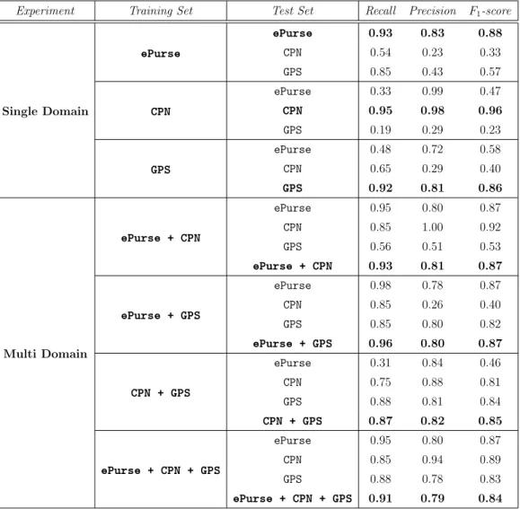
Knauss et al. made a first attempt at classifying security requirements within the SecReq dataset with the Na¨ıve Bayes approach [26]. They conducted two sets of experiments using 10-fold cross-validation for each combination of training and test sets:

1. Single Domain. Train a classifier with one individual SRS and test on another individual SRS.

2. Multi Domain. Train a classifier with a combination of SRS documents and test on an individual SRS.

The experiments are designed to gauge the effectiveness of training a classifier to use in classifying security requirements in different domains, consequently assessing whether overfitting can be avoided.

The results are aggregated in Table 2.7. Knauss et al. deemed a classifier to be useful if it achieves at least 70% recall and 60% precision [26]. Unsurprisingly, all experiments with classifiers trained and tested within the same domain(s) pass the test, whereas almost all the experiments with classifiers tested on an foreign domain do not.

Table 2.7: SecReq Na¨ıve Bayes classification experiments by Knauss et al. [26].

Experiment Training Set Test Set Recall Precision F1-score

Single Domain ePurse ePurse 0.93 0.83 0.88 CPN 0.54 0.23 0.33 GPS 0.85 0.43 0.57 CPN ePurse 0.33 0.99 0.47 CPN 0.95 0.98 0.96 GPS 0.19 0.29 0.23 GPS ePurse 0.48 0.72 0.58 CPN 0.65 0.29 0.40 GPS 0.92 0.81 0.86 Multi Domain ePurse + CPN ePurse 0.95 0.80 0.87 CPN 0.85 1.00 0.92 GPS 0.56 0.51 0.53 ePurse + CPN 0.93 0.81 0.87 ePurse + GPS ePurse 0.98 0.78 0.87 CPN 0.85 0.26 0.40 GPS 0.85 0.80 0.82 ePurse + GPS 0.96 0.80 0.87 CPN + GPS ePurse 0.31 0.84 0.46 CPN 0.75 0.88 0.81 GPS 0.88 0.81 0.84 CPN + GPS 0.87 0.82 0.85 ePurse + CPN + GPS ePurse 0.95 0.80 0.87 CPN 0.85 0.94 0.89 GPS 0.88 0.78 0.83 ePurse + CPN + GPS 0.91 0.79 0.84

2.9.2 Classifying Quality Attributes

Keyword Mining Approach

Cleland-Huang et al. first conducted a small experiment to evaluate how effective a simple keyword mining approach can be when classifying non-functional requirements [14]. The team mined security and performance catalogs to extract sets of keywords associated with security and performance. Requirements containing words from the security keyword set were predicted as security NFRs, and those containing words

from the performance keyword set were predicted as performance NFRs. Require-ments containing words from both were likewise classified as both, and requireRequire-ments containing none were classified as neither.

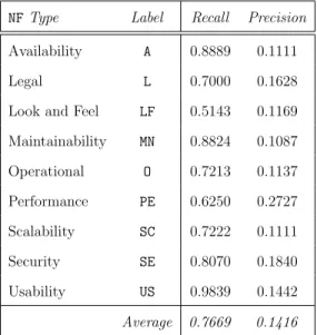
The security classifier scored 79.8% for recall and 56.7% for precision, whereas the performance classifier scored 60.9% for recall and 39.6% for precision. The poor precision is due to the fact that many of these keywords were shared by other types of NFRs. The researchers did not replicate this experiment with any other NFR types due to the difficulty in finding catalogs related to the quality attribute to mine keywords from.

Weighted Indicator Approach

Cleland-Huang et al. next proposed a weighted indicator approach based on informa-tion retrieval to detect and classify NFRs [14]. The classifier is built on an explicit supervised learning-like model with pre-labeled training sets and a manual feature extraction process.

The method is detailed as follows: The requirements are first preprocessed with stop word removal and stemming. Using a pre-labeled training set, indicator terms for each NFR type are then mined and assigned probabilistic weights. Afterward, using the indicator terms, a requirement can be classified as a certain NFR type if its computed probability score beats a chosen threshold.

The researchers ran 15 iterations of the leave-one-out cross-validation technique, partitioning 14 out of the 15 projects to use as the training set and reserving the last project for validation. Table 2.8 showcases the results from selecting the 15 terms with the highest weights as indicator terms and choosing a threshold value of 0.04.

Table 2.8: Results from using top-15 terms at classification with threshold value of 0.04, by Cleland-Huang et al. [14].

NFType Label Recall Precision Availability A 0.8889 0.1111

Legal L 0.7000 0.1628

Look and Feel LF 0.5143 0.1169 Maintainability MN 0.8824 0.1087 Operational O 0.7213 0.1137 Performance PE 0.6250 0.2727 Scalability SC 0.7222 0.1111 Security SE 0.8070 0.1840 Usability US 0.9839 0.1442 Average 0.7669 0.1416

Semi-supervised Learning Approach

Fully-supervised learning requires a large amount of pre-labeled samples for train-ing, meaning analysts need to manually review the requirements and make decisions as to which category the requirement belongs to. In hopes to alleviate such a time consuming prerequisite, Casamayor et al. [11] proposed a semi-supervised learning approach to NFR classification. The approach requires a reduced amount of pre-labeled data by incorporating unpre-labeled data into the learning process through a semi-supervised algorithm called Expectation Maximization (EM), which they built with Bayesian classifiers. They employed theone-vs.-all strategy for multi-label clas-sification, where a binary classifier is trained for each class and during validation, requirements are classified as the class from the binary classifier that produces the highest score.

The requirements documents first undergo normalization, stop word removal, and stemming before being transformed into TF-IDF vectors. Experiments were run using stratified 10-fold cross-validation.

(a) Recall (b) Precision Figure 2.6: Recall and precision results from one-vs.-all multi-label classification of NFR types from Casomayor et al. [11].

.

Casomayor et al. demonstrate that their semi-supervised approach beats the performance of supervised methods like Na¨ıve Bayes, k-nearest neighbors, and TF-IDF. Figure 2.6 showcases the recall and precision scores for one-vs.-all multi-label classification of NFR types over a range of volumes of pre-labeled data.

Chapter 3

DESIGN AND IMPLEMENTATION

To restate our research questions at hand, our goal for this thesis is to evaluate the effect of two deep learning methodologies applied directly to the domain of software requirements documents and the task of requirements classification. Specifically, we aim to investigate the following:

1. RQ1: The feasibility of deep learning models, namely CNNs, on requirements document analysis.

2. RQ2: The efficacy of pre-trained word embeddings in requirements document vectorization.

The unique properties of software requirements documents pose a number of con-cerns when considering deep learning techniques as the nature of the data does not align with the conditions conventionally well-suited for deep learning applications. Specifically, the following attributes of our data pique our interest:

1. Software requirements documents tend to be short in length, resulting in feature-poor data samples. Deep learning analyses typically require feature-rich data, so in the case of text, translates to much lengthier documents.

2. Software requirements datasets tend to be shallow in volume, in the order of hundreds of samples. Deep learning is typically employed to analyze massive volumes of data, in the order of millions or billions.

We want to evaluate whether the usage of feature-rich word representations pro-vided through word embeddings can enrich the features of these documents and make

up for their sparseness. Especially since requirements documents are often character-ized by formal writing and domain-specific jargon, the words that make up the re-quirement text must be key in identifying characteristics of individual rere-quirements. Since word embeddings are claimed to preserve semantic relationships between words that are otherwise lost in traditional vectorization methods such as TF-IDF [34, 35], we want to investigate whether these advantages can counteract the feature-poor quality of requirements samples.

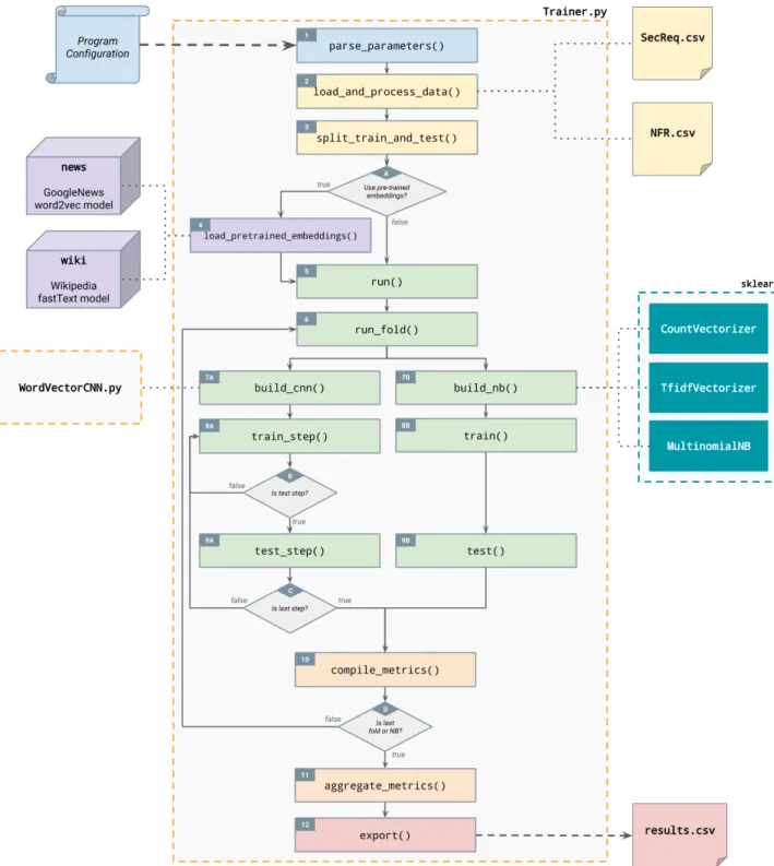
In order to study these inquiries, we needed to design an instrument that can orchestrate the data preparation, classifier training, and performance evaluation nec-essary to assess the impact of the technologies mentioned above against our concerns with the nature of our domain. We built such a system with the help of machine learning tools such as TensorFlow, Scikit-Learn, Gensim, and NLTK. Figure 3.1 show-cases an activity diagram that breaks down the operation flow within our system. The system features one flow to train a Na¨ıve Bayes classifier using Scikit-Learn’s MultinomialNB1 implementation, as well as a flow to train a one-layer text classifica-tion CNN modeled after the sentence classificaclassifica-tion CNN design proposed by Kim et al. [23] and illustrated in Figure 2.4. The following sections walk through the steps of the activity diagram, further discussing each operation in detail.

3.1 Run Configurations

Our system accepts a set of command line configurations (or parameters) for each experiment run, categorized and detailed in Table 3.1. The program configurations are parsed in Block 1 of the activity diagram in Figure 3.1.

1

Table 3.1: Run configuration options.

Category Configuration Type Description

Dataset

Training Set str Dataset for training. Test Set str Dataset for testing. Label(s) set(str) Label(s) to classify.

Validation

Cross-Validation bool Whether to runk-fold cross-validation.

# of Folds (k) int Ifk-fold cross-validation is set, specifyk(e.g., 10).

Test Percentage float Ifk-fold cross-validation is not set, specify % of dataset reserved for test (e.g., 0.25).

Preprocessing

Stratification bool Whether to stratify the training and test sets. Stop Word Removal bool Whether to remove stop words from the corpora.

Lemmatization bool Whether to lemmatize the corpora.

Classifier

CNN bool Whether to train a CNN classifier.

Embeddings str Word embedding initialization ("random","w2v", or"fasttext"). Filter Sizes set(int) Set of filter sizes (e.g.,{1,2,3}).

# of Filters int Number of filters per filter size (e.g., 128). # of Epochs int Number of epochs to train for (e.g., 140).

NB bool Whether to train a NB classifier.

Vectorizer str Vectorization method ("count"or"tfidf"). Program Seed int Seed to control randomization (e.g., 42).

3.2 Data Loading and Preprocessing

Next in the pipeline, the data is loaded and preprocessed (according to the program configurations) and converted into a uniform data format for our classifiers to accept. This occurs in Block 2 of the activity diagram in Figure 3.1.

3.2.1 Raw Data Formats

As the SecReq and NFR datasets come in different formats, we discuss processing both dataset separately.

SecReq

The SecReq dataset is comprised of three different SRS documents in the form of three similarly formatted semicolon-delimited CSV files: ePurse-selective.csv,

The CNG shall support mechanisms to authenticate itself to the NGN for connectivity purposes.;sec

(a) Security-related

The CND should be able to support bootstrap capabilities in order to retrieve network configuration data to connect the NGN.;nonsec

(b) Not security-related

Figure 3.2: Examples of SecReq raw data format.

CPN.csv, and GPS.csv. Each data point in the collection features two attributes: the requirements text and the requirements class label (sec or nonsec). Figure 3.2a showcases an example of a security-related requirement, whe