Substructural Analysis Using Evolutionary Computing Techniques
By:
Nor Samsiah Binti Sani
A thesis submitted in partial fulfilment of the requirements for the degree of Doctor of Philosophy
The University of Sheffield Faculty of Social Sciences
School of Information
ii
Acknowledgments
First and foremost, I would like to thank my supervisors Professor Peter Willett and Dr John Holliday for their constant supervision and guidance during this PhD study, and also during the writing up of this thesis. I can‟t thank you enough for all the fruitful discussions and advices given in the throughout the research. I would like to thank all the staff, colleagues and members of the University of Sheffield‟s Chemical Information System Research Group (CISRG) for their kindness and support during the course of this work. Not forgetting Dr Sudholt from the University of Sheffield‟s School of Computer Science for his valuable insights and discussions on evolutionary algorithms.
I would like to convey my deepest thanks to my whole family members in Malaysia, especially my parents (Hj Sani Ithnin and Hjh Artini Dayat) and my parents-in-law (Hj Azmi Anuar and Hjh Ungku Mariam) for their love, care and constant prayer for my success. To both my siblings, Nor Suriani and Mohd Aliff Afira, for their never-ending words of encouragements. Special appreciation to my husband Ahmad Kamal Azmi, the one whom have persistently given me strength, motivation, encouragements when needed, and sometimes when all else fails, just practically a shoulder to lean on. To my children, Arissa Humaira and Adam Ashraf, you both cheer me up constantly no matter how busy I get, and I truly appreciate it. I would never have made this far without their support and love. I would like to dedicate this achievement to all of you.
I would also like to thank my main sponsors: The Ministry of Higher Education (MOHE), Malaysia and also my employer, Universiti Kebangsaan Malaysia (UKM) for the opportunity given in pursuant of this PhD study. Thank you.
iii
Abstract
Substructural analysis (SSA) was one of the very first machine learning techniques to be applied to chemoinformatics in the area of virtual screening. For this method, given a set of compounds typically defined by their fragment occurrence data (such as 2D fingerprints). The SSA computes weights for each of the fragments which outlines its contribution to the activity (or inactivity) of compounds containing that fragment. The overall probability of activity for a compound is then computed by summing up or combining the weights for the fragments present in the compound. A variety of weighting schemes based on specific relationship-bound equations are available for this purpose. This thesis identifies uplift to the effectiveness of SSA, using two evolutionary computation methods based on genetic traits, particularly the genetic algorithm (GA) and genetic programming (GP). Building on previous studies, it was possible to analyse and compare ten published SSA weighting schemes based on a simulated virtual screening experiment. The analysis showed the most effective weighting scheme to be the R4 equation which was a part of document-based weighting schemes. A second experiment was carried out to investigate the application of GA-based weighting scheme for the SSA in comparison to an experiment using the R4 weighting scheme. The GA algorithm is simple in concept focusing purely on suitable weight generation and effective in operation. The findings show that the GA-based SSA is superior to the R4-based SSA, both in terms of active compound retrieval rate and predictive performance. A third experiment investigated the genetic application via a GP-based SSA. Rigorous experiment results showed that the GP was found to be superior to the existing SSA weighting schemes. In general, however, the GP-based SSA was found to be less effective than the GA-based SSA. A final experimented is described in this thesis which sought to explore the feasibility of data fusion on both the GA and GP. It is a method producing a final ranking list from multiple sets of ranking lists, based on several fusion rules. The results indicate that data fusion is a good method to boost GA-and GP-based SSA searching. The RKP rule was considered the most effective fusion rule.
iv
Table of Contents
Acknowledgments ... ..ii Abstract……….…….iii Table of Contents ... iv List of Figures ... xList of Tables ………..xvii
CHAPTER 1: Introduction
1.1 The drug discovery process ... 11.2 Chemoinformatics and the use of machine learning methods ... 3
1.3 Research aim and objectives ... 5
1.4 Thesis outline ... 6
CHAPTER 2: Virtual Screening and Substructural Analysis
2.1 Introduction ... 72.2 Representation of chemical structures ... 7
2.2.1 Connection tables ... 7
2.2.2 Morgan algorithm ... 8
2.2.3 Line notation ... 10
2.2.4 Wiswesser Line Notation (WLN) ... 11
2.2.5 Simplified Molecular Input Line Entry System (SMILES) ... 11
2.2.6 International Chemical Identifier (InChI) ... 12
2.3 Molecular descriptors ... 14
2.4 2D descriptors ... 16
2.4.1 Topological indices ... 16
2.4.2 Fragment-based descriptors ... 16
2.5 Searching databases of molecules ... 20
2.5.1 Structure searching ... 20
2.5.2 Substructure searching ... 21
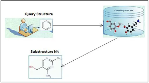
2.5.3 Similarity searching ... 22
v 2.7 Structure-Activity Relationship (SAR) and Quantitative Structure-Activity
Relationship (QSAR) ... 27
2.8 Machine learning ... 30
2.9 Substructural analysis ... 35
2.9.1 History and definition ... 35
2.9.2 Fundamental components of the SSA ... 35
2.9.3 The SSA weighting schemes ... 37
2.10 Application of SSA for drug discovery ... 44
2.10.1 Hodes study in National Cancer Institute (NCI) for tumour screening program 45 2.10.2 CASE and MULTICASE ... 46
2.10.3 SLASH ... 47
2.10.4 Other applications of SSA ... 47
2.11 SSA and Naive Bayesian Classifier (NBC) ... 48
2.12 Performance evaluation and validation for SSA ... 51
2.13 Conclusion ... 52
CHAPTER 3: Research Methodology
3.1 Introduction ... 55 3.2 Datasets ... 55 3.2.1 MDDR ... 55 3.2.2 WOMBAT ... 56 3.2.3 ChEMBL ... 56 3.3 Fingerprints ... 583.4 Test set and training set ... 59
3.5 SSA weighting schemes evaluation methods ... 62
3.5.1 Enrichment Factor (EF) ... 63
3.5.2 Analysis of diversity ... 64
3.5.3 Statistical tests ... 65
3.5.3.1 Kendall‟s W analysis ... 65
3.5.3.2 Wilcoxon signed rank test ... 66
3.6 Hardware ... 68
vi
CHAPTER 4: The Comparison of Different Weighting Schemes in
Substructural Analysis Using Large Datasets
4.1 Introduction ... 70
4.2 Experimental details ... 70
4.3 Experimental procedure ... 70
4.3.1 Weighting schemes ... 71
4.3.2 Benchmarking SSA performance against NBC Pipeline Pilot ... 71
4.4 Analysis of SSA weighting schemes ... 71
4.4.1 Enrichment curve analysis ... 72
4.4.2 Kendall‟s W analysis ... 73
4.4.3 Analysis of the SSA R4 fragment weights ... 76
4.5 Discussion ... 78
4.6 Conclusion ... 80
CHAPTER 5: Genetic Algorithm Approach to Substructural Analysis
5.1 Introduction ... 965.2 Fundamental components of GA for SSA ... 96
5.2.1 Encoding of chromosomes ... 97
5.2.2 Fitness criterion ... 98
5.2.3 Chromosome selection methods for genetic operations ... 98
5.2.4 Evolutionary operators ... 99
5.2.5 Chromosome‟s principle of elitism ... 100
Simple-state preservation model ... 101
Steady-state preservation model ... 101
5.3 Previous works in GA... 102
5.4 Experiment details ... 104
5.4.1 Dataset ... 104
5.4.2 Hardware ... 104
5.4.3 Algorithm implementation ... 105
5.4.3.1 Suitable fitness function for SSA–based GA ... 106
5.3.3.2 Weight polarity to overcome overfitting ... 108
5.4.3.3 Selection of chromosomes and genetic operations ... 111
vii
5.6 Experiment setup: Parameterisation of GA-based SSA ... 115
5.6.1 Fitness function ... 116
5.6.2 GA weight range of chromosomes ... 117
5.6.3 Population size and generations of evolution ... 117
5.6.4 Elitism model ... 119
5.6.5 Evolution control ... 119
5.6.6 Final parameterisation selections ... 120
5.7 Experiment result: Analysis of performance of GA-based SSA ... 121
5.7.1 GA robustness ... 121
5.7.2 GA weights correlation and consistency of compounds retrieval ... 122
5.7.3 Analysis of GA runs on all activity classes ... 123
5.7.3.1 Enrichment curve analysis ... 123
5.7.3.2 Analysis of diversity ... 124
5.7.4 Wilcoxon signed rank test ... 125
5.7.5 Model validation with Y-randomisation ... 125
5.7.6 Run-time benchmarks of GA-based SSA ... 127
5.8 Discussion ... 128
5.9 Conclusion ... 129
CHAPTER 6: Genetic Programming Approach to Substructural Analysis
6.1 Introduction ... 1596.2 Fundamental components of GP for SSA ... 159
6.2.1 Encoding of Chromosomes ... 161 6.2.2 Population growth ... 162 6.2.3 Evolutionary operators ... 163 6.3 Previous works in GP ... 163 6.4 Experimental details ... 164 6.4.1 Dataset ... 164 6.4.2 Hardware ... 164 6.4.3 Algorithm Implementation ... 165
6.4.3.1 Chromosomes population and generation ... 165
6.4.3.2 Suitable fitness function design for GP-based SSA ... 167
viii
6.6 Experiment setup: Parameterisation of the GP-based SSA ... 168
6.6.1 Fitness function ... 169
6.6.2 Terminal and function sets for chromosome generation ... 170
6.6.3 Chromosome structure ... 171
6.6.4 Population size, generation and tree properties ... 172
6.6.5 Elitism model ... 173
6.6.6 Evolution control ... 174
6.6.7 Final parameterisation selections ... 174
6.7 Experiment result: Analysis of the performance of GP-based SSA ... 175
6.7.1 GP robustness ... 175
6.7.2 GP weights correlation and consistency of compounds ... 176
6.7.3 Analysis of GP runs on all activity classes ... 177
6.7.3.1 Enrichment curve analysis ... 178
6.7.3.2 Analysis of diversity ... 179
6.7.4 Kendall‟s W analysis ... 179
6.7.5 Wilcoxon signed rank test ... 180
6.7.6 GP-generated equations ... 181
6.7.7 Model validation with Y-randomisation ... 181
6.7.8 Run-time benchmarks of GP-based SSA ... 183
6.8 Discussion ... 184
6.9 Conclusion ... 185
CHAPRER 7: Investigations Into The Application of Data Fusion
7.1 Introduction ... 2287.2 Data fusion ... 228
7.3 Experimental details ... 230
7.3.1 Datasets ... 230
7.3.2 Fusion rules ... 230
7.4 Results and discussion ... 232
7.4.1 GA and GP-based fusion performance analysis ... 232
7.4.2 Kendall‟s W analysis ... 233
7.4.3 Wilcoxon signed rank test ... 235
ix
CHAPTER 8: Conclusion and Future Work
8.1 Introduction ... 247
8.2 Contributions ... 248
8.2.1 The comparison of existing SSA weighting schemes ... 248
8.2.2 The use of GA to the SSA method ... 249
8.2.3 Investigation of the use of GP in the SSA method ... 250
8.2.4 Investigation into the use of data fusion to the GA-and GP-based SSA ... 251
8.3 Suggestion for future work ... 251
8.4 Conclusion ... 252
Appendix A: The GA-based SSA pseudocode ... 254
Appendix B: The GP-based SSA pseudocode ... 256
x
List of Figures
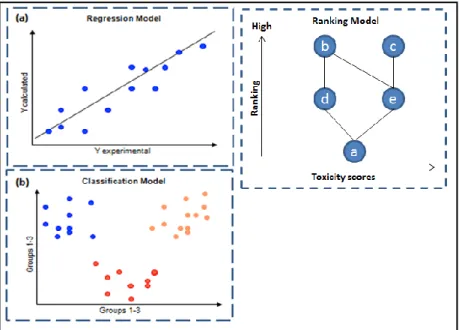
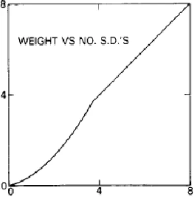
Figure 1.1: Trends in pharmaceutical research for drug discovery and design (after Terstappen and Reggiani, 2001) ... 2 Figure 2.1: Connection table representation (after Leach & Gillet, 2007). Information such as atom coordinates relating to its formation and bonding pairs are stored for accurate rebuilding of the molecules ... 8 Figure 2.2: Morgan algorithm procedure (after Leach & Gillet, 2007) ... 9 Figure 2.3: Canonical state of structure for computer representation (adapted from UTM open courseware chemistry website) ... 11 Figure 2.4: 2D chemical structure (left) and structural key fingerprint (right) ... 17 Figure 2.5: Graph A and B are isomorphic and topologically identical (after Yirka, 2015) .... 21 Figure 2.6: Schema of chemical substructure searches (after Horai et al., 2010) ... 22 Figure 2.7: Overview of typical screening process (after Lengauer, Lemmen, Rarey, & Zimmermann, 2004) ... 25 Figure 2.8: Different types of QSAR strategies (after Todeschini & Consonni, 2008): (a) Regression model focusing on the best fit classifications; (b) Classification model to characterise the similarity between certain properties, and (c) Partial order ranking models, based on Hasse diagram technique. The figure shows the ranks of chemicals according to their toxicity levels, which relies on statistical significance ... 28 Figure 2.9: Simple schematics of Substructural Analysis ... 36 Figure 2.10: Plot of weight versus number of standard deviation with conversion to log 1/P (Hodes et al., 1977) ... 41 Figure 3.1: (a) A molecule from the ChEMBL database and (b) Its corresponding Murcko scaffold ... 58 Figure 3.2: Pipeline Pilot workflow for fingerprint ... 59
xi Figure 4.1: Methodology of experimental procedures conducted in predictive analysis ... 82 Figure 4.2: Pipeline Pilot workflow to generate NBC models using training sets... 82 Figure 4.3: Pipeline Pilot workflow for new candidate screening using generated NBC models ... 82 Figure 4.4: Cumulative recall plots of the various SSA weighting schemes for the 5HT3 activity class from the (a) MDDR (b) WOMBAT and (c) ChEMBL dataset ... 83 Figure 4.5: Cumulative recall plots of the various SSA weighting schemes for the COX activity class from the (a) MDDR (b) WOMBAT and (c) ChEMBL dataset ... 84 Figure 4.6: Cumulative recall plots of the various SSA weighting schemes for the D2 activity class from the (a) MDDR (b) WOMBAT and (c) ChEMBL dataset ... 85 Figure 4.7: Cumulative recall plots of the various SSA weighting schemes for the RNN activity class from the (a) MDDR (b) WOMBAT and (c) ChEMBL dataset ... 86 Figure 4.8: Cumulative recall plots of the various SSA weighting schemes for the PKC activity class from the (a) MDDR (b) WOMBAT and (c) ChEMBL dataset ... 87 Figure 4.9: Comparison of the eleven MDDR activity classes based on the enrichment factor of actives in the top 1% of the rankings ... 88 Figure 4.10: Comparison of the fourteen WOMBAT activity classes based on the enrichment factor of actives in the top 1% of the rankings ... 88 Figure 4.11: Comparison of the fifteen ChEMBL activity classes based on the enrichment factor of actives in the top 1% of the ranking ... 89 Figure 4.12: Comparison of fragment weights of 166 fragments, at m equals 0.0000001, 0.01, 0.05, 0.1 and 0.5. The SSA R4 weights are computed using the training sets of predictive analysis of COX activity class in the MDDR database ... 89 Figure 5.1: The basic genetic algorithm flowchart ... 131 Figure 5.2: Roulette wheel selection after Goldberg (1987). (a) Outlines a set of evaluated chromosomes with different fitness scores, and their relative percentage of the total fitness.
xii (b) The chromosomes are sorted and fitted into a roulette wheel model where larger chromosomes take a bigger portion of the wheel. A random number generated ranging from 0 to 100% will iterate through the wheel until the value is achieved, thus selecting the parent chromosome ... 132 Figure 5.3: Tournament selection. (a) Four chromosomes are selected at random and assigned as paired opponents. Fitness scores are observed between opponents and the winner progresses to the next round. (b) The winners of round 1 pitted against one another in round 2 by observing their fitness score. (c) The winner of round 2 is selected as the parent chromosome for the next genetic operation. This process is repeated to select the other parent chromosome as genetic operation requires two parents to proceed ... 132 Figure 5.4: Genetic operations in the genetic algorithm. (a) A population list consisting of chromosomes represented as bit-strings. (b) Two parent chromosomes selected from the population list to perform a crossover operation, which takes a portion of each chromosome‟s genes and recombines them into a single, new chromosome. (c) Mutation operation flips a random bit of the chromosome. (d) Child chromosome inserted back into the population list ... 133 Figure 5.5: Crossover methods in the GA. (a) One point crossover method; (b) Two points crossover, and (c) Uniform crossover ... 133 Figure 5.6: Simple-state elitism model with six chromosomes created at initialisation. After going through reproduction process, each generation concludes with modification to the population. In this case, an elitism of two parents ensures that all the chromosomes are replaced through genetic operations except for the two best parent chromosomes ... 134 Figure 5.7: Steady-state elitism model with six chromosomes created at initialisation. During the replacement process only one chromosome, being the worst performing one, is replaced with a reproduced, offspring chromosome. The remaining chromosomes are maintained, which is also known as the overlapping population method ... 134 Figure 5.8: The genetic algorithm flowchart with inclusion of weight polarity constraining operations. The GA assumes normal operation except that the weight polarity needs to be identified first, and both the population initialisation and subsequent genetic operations include conditional weight assignment based on the polarity criterion ... 135
xiii Figure 5.9: Cumulative recall plots of the GA-based SSA against SSA R4 for the RNN activity class from the MDDR dataset based on the different fitness function (a) In the top 1%; and (b) In top 10% of ranked compounds... 136 Figure 5.10: Cumulative recall plots of the GA-based SSA against SSA R4 for the COX activity class from the MDDR dataset based on the different fitness function (a) In the top 1%; and (b) In top 10% of ranked compounds... 137 Figure 5.11: Error plot of training set versus predicted test set of the GA-based SSA following GA iterations for MDDR (a) RNN and (b) COX activity classes. Both GA instances were executed based on a chromosome population of 200 and maximum iteration of 500 to signify (i) Overfitting case, and (ii) Presence of improved recall rates in large iterations... 138 Figure 5.12: The cumulative recall of active compounds plotted against the entire compound over 10 runs of the GA program: (a) GA instances for MDDR-based RNN activity class; (b) GA instances for MDDR-based COX activity class ... 139 Figure 5.13: Cumulative recall plots of the GA-based SSA against SSA R4 for the 5HT3 activity class from the (a) MDDR (b) WOMBAT and (c) ChEMBL dataset. Plots represent the worst performing run of each method ... 140 Figure 5.14: Cumulative recall plots of the GA-based SSA against SSA R4 for the COX activity class from the (a) MDDR (b) WOMBAT and (c) ChEMBL dataset. Plots represent the worst performing run of each method ... 141 Figure 5.15: Cumulative recall plots of the GA-based SSA against SSA R4 for the D2 activity class from the (a) MDDR (b) WOMBAT and (c) ChEMBL dataset. Plots represent the worst performing run of each method ... 142 Figure 5.16: Cumulative recall plots of the GA-based SSA against SSA R4 for the RNN activity class from the (a) MDDR (b) WOMBAT and (c) ChEMBL dataset. Plots represent the worst performing run of each method ... 143 Figure 5.17: Cumulative recall plots of the GA-based SSA against SSA R4 for the PKC activity class from the (a) MDDR (b) WOMBAT and (c) ChEMBL dataset. Plots represent the worst performing run of each method ... 144
xiv Figure 5.18: Permutation plots (Y-randomisation) of the MDDR-based (a) RNN and (b) COX classes, with weights calculated and applied to non-permuted test sets ... 145 Figure 6.1: Genetic programming basic flow, (after Poli, Langdorn, McPhee & Koza, 2008) ... 187 Figure 6.2: Simple structure of a tree model in GP, (a) a valid tree model compared to (b) invalid tree with incomplete equation portion in its child branch, highlighted in red ... 187 Figure 6.3: Chromosome tree creation using the grow method. Tree defined with a maximum depth of 3 levels ... 188 Figure 6.4: Chromosome tree creation using the full method. Tree defined with a maximum of 3 levels of tree depth ... 188 Figure 6.5: GP's crossover operation diagram ... 189 Figure 6.6: GP‟s mutation example showing the (a) Single terminal mutation, and (b) Sub-tree mutation ... 189 Figure 6.7: A GP equation producing chaotic fragment weights of inappropriate large values. The multiplication of a large variable TOT with itself while enhanced by the accompanying exponential term causes a number of weights to be significantly larger in value ... 190 Figure 6.8: An equation from Figure 6.7 now wrapped by a mandatory log function generates much smaller weight values ... 190 Figure 6.9: GP representation of chromosomes towards fitness determination. (a) A training set made up of compounds via 2D fingerprints description. (b) A GP population representing chromosome equations made up of parameters to explain training set. (c) Chromosome chr1 is translated from the equation form to weight values, applied to training set to determine compound score. (d) Compounds are ranked in descending order. (e) Fitness of chromosome is calculated as the rate of the active retrieval in the top percentile of the ranked compounds set ... 191 Figure 6.10: Cumulative recall plots of the GP-based SSA against SSA R4 for the RNN activity class from the MDDR dataset based on the different fitness function in (a) The top 1%; and in (b) The top 10% of ranked compounds ... 192
xv Figure 6.11: Cumulative recall plots of the GP-based SSA against SSA R4 for the COX activity class from the MDDR dataset based on the different fitness function in (a) The top 1%; and in (b) The top 10% of ranked compounds ... 193 Figure 6.12: Error plot of training set versus predicted test set of the GP-based SSA for MDDR RNN activity class, based on (a) VARIABLES_A set only, and (b) VARIABLES_A and VARIABLES_B combination ... 194 Figure 6.13: Error plot of training set versus predicted test set of the GP-based SSA for MDDR COX activity class, based on (a) VARIABLES_A set only, and (b) VARIABLES_A and VARIABLES_B combination ... 194 Figure 6.14: The Cumulative recall of active compounds plotted against the entire compound over 10 runs of the GP program: (a) GP instances for MDDR-based RNN activity class; (b) GP instances for MDDR-based COX activity class ... 195 Figure 6.15: Cumulative recall plots of the GP-based SSA against SSA R4 and GA-based SSA for 5HT3 activity class for the (a) MDDR (b) WOMBAT and (c) ChEMBL dataset. Plots represent the worst performing run of each method ... 196 Figure 6.16: Cumulative recall plots of the GP-based SSA against SSA R4 and GA-based SSA for COX activity class for the (a) MDDR (b) WOMBAT and (c) ChEMBL dataset. Plots represent the worst performing run of each method ... 197 Figure 6.17: Cumulative recall plots of the GP-based SSA against SSA R4 and GA-based SSA for D2 activity class for the (a) MDDR (b) WOMBAT and (c) ChEMBL dataset. Plots represent the worst performing run of each method ... 198 Figure 6.18: Cumulative recall plots of the GP-based SSA against SSA R4 and GA-based SSA for RNN activity class for the (a) MDDR (b) WOMBAT and (c) ChEMBL dataset. Plots represent the worst performing run of each method ... 199 Figure 6.19: Cumulative recall plots of the GP-based SSA against SSA R4 and GA-based SSA for PKC activity class for the (a) MDDR (b) WOMBAT and (c) ChEMBL dataset. Plots represent the worst performing run of each method ... 200
xvi Figure 6.20: Permutation plots (Y-randomisation) of the MDDR-based (a) RNN and (b) COX classes, with weights calculated and applied to non-permuted test sets ... 201 Figure 6.21: Example of a GP-based SSA (a) Original equation and (b) The simplified equation using Wolfram Alpha expression simplifier online tool ... 202
xvii
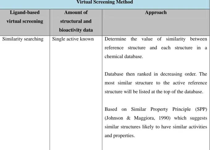
List of Tables
Table 2.1: Linear chemical notation ... 14 Table 2.2: Approaches in ligand-based and structure-based virtual screening... 26 Table 2.3: Comparison of machine learning classification techniques in LBVS (after Lavecchia, 2015) ... 32 Table 2.4: Summary of past performance evaluation programs on SSA ... 53 Table 3.1: (a) MDDR, (b) WOMBAT and (c) ChEMBL activity classes considered in this study ... 60 Table 3.2: Computer‟s hardware specification used to run the GA-based SSA. (a) Server setup; (b) Multimedia-intensive workstation; (c) Office-level workstation; and (d) Laptop setup ... 69 Table 4.1: Enrichment factor of actives retrieved in the top 1% of the ranked compounds of (a) The eleven activity class in MDDR (b) The fourteen activity class in WOMBAT dataset, and (c) The fifteen activity classes in ChEMBL dataset ... 90 Table 4.2: Kendall's W analysis for the top 1% actives retrieved of the ranking for (a) Eleven activity classes in MDDR, (b) Fourteen activity classes in WOMBAT, and (c) Fifteen activity classes of the ChEMBL database ... 92 Table 4.3: Kendall's W analysis for the top 1% based on the average of enrichment factor actives in the top 1% from the MDDR, WOMBAT and ChEMBL databases ... 93 Table 4.4: Fragment weights computed using R4 function for fourteen fragments (1, 2, 5, 19, 13, 17, 74, 67, 38, 53, 166, 164, 127 and 154) at m equals to 0.0000001, 0.01, 0.05, 0.1 and 0.5. The weights were derived using training sets in the predictive analysis ... 94 Table 4.5: Statistics for 166 fragment weights for m equals 0.0000001, 0.01, 0.05, 0.1 and 0.5. The SSA R4 fragment weights are derived using the training set of predictive analysis of COX activity classes in the MDDR database ... 95
xviii Table 5.1: Example of a GA operation based on a population containing five molecules, with six chromosomes created at initialisation. (a) Fingerprints for five molecules M1-5 encoding five different substructural fragments F1-5; (b) The molecule activity state, 1 referring to an active molecule, while 0 represents inactive ones. (c) Six chromosomes C1-6 encoding the
weights W1-5 for F1-5; and (d) Sums-of-weights using each chromosome C1-6 for each molecule
M1-5 ... 146
Table 5.2: Weight polarity determination using the SSA R4 weighting scheme, following the example molecule and activity dataset in Table 5.1. (a) Summary of a five-fragment dictionary based on the common properties in SSA weighting schemes. (b) Weight polarity for fragments is determined on the basis of greater value between the rate-of-actives (ROA) against the rate-of-inactives (ROI). (c) The equivalent weight values and its polarity calculated using the SSA R4 weighting scheme ... 147 Table 5.3: Fitness score calculation using chromosome C3 with its weights restricted by the
weight polarity. (a) Chromosome C1 weights combination and the corresponding weight
polarity. (b) Assignment of chromosome weight to each fragment in the molecule set. (c) Sum of fragments‟ score of each molecule. (d) Ranking of chromosome based on molecule score in descending order from largest to smallest. All the active molecules are seen to benefit from SSA R4 weight polarity assignment based on their rankings at the top ... 148 Table 5.4: Top 1% active retrieval rates for the fitness function parameter test. Listed are test set enrichment values for MDDR‟s RNN and COX activity classes. GAs were performed on training set of 10% active and inactive compounds, where the resultant weights are subsequently applied on the predicted test set of 90% active and inactive compounds. The worst enrichment values of 3 GA runs are listed below. Each parameter was executed three times and the worst result is selected to represent the individual parameters. ... 149 Table 5.5: Top 1% active retrieval rates for the GA weight range parameter group. Listed are test set enrichment values for MDDR‟s RNN and COX activity classes. GAs were performed on training set of 10% active and inactive compounds, where the resultant weights are subsequently applied on the predicted test set of 90% active and inactive compounds. The worst enrichment values of 3 GA runs are listed below. Each parameter was executed three times and the worst result is selected to represent the individual parameters. ... 149
xix Table 5.6: Top 1% active retrieval rates for the GA Population and Generation parameter group. Listed are test set enrichment values for MDDR‟s RNN and COX activity classes. GAs were performed on training set of 10% active and inactive compounds, where the resultant weights are subsequently applied on the predicted test set of 90% active and inactive compounds. The worst enrichment values of 3 GA runs are listed below. Each parameter was executed three times and the worst result is selected to represent the individual parameters 150 Table 5.7: Top 1% active retrieval rates for the elitism model parameter. Listed are test set enrichment values for MDDR‟s RNN and COX activity classes. GAs were performed on training set of 10% active and inactive compounds, where the resultant weights are subsequently applied on the predicted test set of 90% active and inactive compounds. The worst enrichment values of 3 GA runs are listed below. Each parameter was executed three times and the worst result is selected to represent the individual parameters ... 151 Table 5.8: Top 1% active retrieval rates for the evolution control parameter group. Listed are test set enrichment values for MDDR‟s RNN and COX activity classes. GAs were performed on training set of 10% active and inactive compounds, where the resultant weights are subsequently applied on the predicted test set of 90% active and inactive compounds. The worst enrichment values of 3 GA runs are listed below. Each parameter was executed three times and the worst result is selected to represent the individual parameters ... 152 Table 5.9: The top-ranked molecules in ten GA runs based on test set applied data, showing the occurrences of ranked compounds based on GA run-1 that fall outside the top 1% in the other nine remaining GA runs using the (a) RNN and (b) COX activity classes in the MDDR dataset. The numbers in brackets show the number of actives actually retrieved in the top 1% for that particular GA-run ... 153 Table 5.10: Enrichment curve of actives count in the top 1% for ten GA runs of (a) Eleven activity classes in MDDR dataset; (b) Fourteen activity classes in WOMBAT dataset and; (b) Fifteen activity classes in ChEMBL dataset. Included are the mean and standard deviation for the Pearson correlation coefficients between the sets of 166 weights computed for each distinct pair of runs ... 154 Table 5.11: Screening results using the GA-based SSA and its comparison to the SSA R4 weighting scheme for the (a) MDDR; (b) WOMBAT and (c) ChEMBL datasets. The number of actives retrieved at the top 1% based on the worst performing GA runs is recorded for the
xx calculation of Tanimoto coefficient and the BemisMurckoAssemblies based diversity analysis ... 156 Table 5.12: GA run-time benchmark at different iterations using the 10% training set of the RNN activity class, based on the (a) MDDR, (b) WOMBAT and (c) ChEMBL databases. Parameterisation of the GA is based on the final chosen ones as in Section 5.7.5, among them the population of 200 chromosomes, and a maximum iteration 200 evolutions ... 158 Table 6.1: Summary of differences between GA and GP ... 203 Table 6.2: Top 1% active retrieval rates for the GP fitness function definition test. Listed are test set enrichment values for MDDR‟s RNN and COX activity classes. GPs were performed on a training set of 10% active and inactive compounds, where the resultant weights are subsequently applied on the predicted test set of 90% active and inactive compounds. Each parameter was executed three times and the worst result is selected to represent the individual parameters. The best parameter value is shaded ... 204 Table 6.3: Terminal and function variable combinations used for chromosome initialisation. (a) List of tested variable combinations defined for the GP chromosome terminal set; (b) List of tested operator functions for the GP chromosome function set ... 205 Table 6.4: Top 1% active retrieval rates for the GP terminal and function set combination test. Listed are test set enrichment values for MDDR‟s RNN and COX activity classes. GPs were performed on a training set of 10% active and inactive compounds, where the resultant weights are subsequently applied on the predicted test set of 90% active and inactive compounds. Each parameter was executed three times and the worst result is selected to represent the individual parameters. The best parameter value is shaded... 206 Table 6.5: Top 1% active retrieval rates for the GP‟s chromosome structure tests. Listed are test set enrichment values for MDDR‟s RNN and COX activity classes. Each parameter‟s tree depth and node size values obtained are listed as well. The GPs was performed on a training set of 10% active and inactive compounds, where the resultant weights are subsequently applied on the predicted test set of 90% active and inactive compounds. Each parameter was executed three times and the worst result is selected to represent the individual parameters. The best parameter value is shaded ... 207
xxi Table 6.6: Top 1% active retrieval rates for the GP‟s population and generation based parameter tests. Listed are test set enrichment values for MDDR‟s RNN and COX activity classes. GAs were performed on a training set of 10% active and inactive compounds, where the resultant weights are subsequently applied on the predicted test set of 90% active and inactive compounds. Each parameter was executed three times and the worst result is selected to represent the individual parameters. The best parameter value is shaded ... 208 Table 6.7: Top 1% active retrieval rates for the GP‟s elitism model parameter tests. Listed are test set enrichment values for MDDR‟s RNN and COX activity classes. GPs were performed on a training set of 10% active and inactive compounds, where the resultant weights are subsequently applied on the predicted test set of 90% active and inactive compounds. Each parameter was executed three times and the worst result is selected to represent the individual parameters. The best parameter value is shaded ... 209 Table 6.8: Top 1% active retrieval rates for the GP‟s evolution control parameter tests. Listed are test set enrichment values for MDDR‟s RNN and COX activity classes. GPs were performed on a training set of 10% active and inactive compounds, where the resultant weights are subsequently applied on the predicted test set of 90% active and inactive compounds. Each parameter was executed three times and the worst result is selected to represent the individual parameters. The best parameter value is shaded... 210 Table 6.9: The top-ranked molecules in ten GP runs based on test set applied data, showing the occurrences of ranked active compounds based on GP run-1 that fall outside the top 1% in the other nine remaining GP runs using the (a) RNN and (b) COX activity classes in the MDDR dataset. The numbers in brackets show the number of actives actually retrieved in the top 1% for that particular GP-run ... 211 Table 6.10: Enrichment curve of actives count in the top 1% for ten GP runs of (a) Eleven activity classes in MDDR dataset; (b) Fourteen activity classes in WOMBAT dataset and; (b) Fifteen activity classes in ChEMBL dataset. Included are the mean and standard deviation for the Pearson correlation coefficients between the sets of 166 weights computed for each distinct pair of runs ... 212 Table 6.11: Screening results using the GP-based SSA and its comparison to the SSA R4 and GA-based SSA weighting scheme for the (a) MDDR; (b) WOMBAT and (c) ChEMBL datasets. The number of actives retrieved at the top 1% based on the worst performing GA
xxii runs is recorded for the calculation of Tanimoto coefficient and the BemisMurckoAssemblies based diversity analysis ... 214 Table 6.12: Kendall's W analysis for the top 1% actives retrieved of the ranking for (a) Eleven activity classes in MDDR, (b) Fourteen activity classes in WOMBAT, and (c) Fifteen activity classes of the ChEMBL database ... 217 Table 6.13: The worst and best performing GP equations selected from the 10 runs of each activity class, based on the (a) MDDR, (b) WOMBAT, and (c) ChEMBL18 datasets. All equations are simplified from its original form ... 218 Table 6.14: GP run-time benchmark at different iterations using the 10% training set of the RNN activity class, based on the (a) MDDR, (b) WOMBAT and (c) ChEMBL databases. Parameterisation of the GP is based on the final chosen ones as in Section 6.6.1.6, among them the population of 200 chromosomes, and a maximum iteration 200 evolutions ... 227 Table 7.1: Enrichment factor of actives when using combination of different GA runs for top 1% in (a) MDDR dataset for eleven activity classes (b) WOMBAT dataset for fourteen activity classes and (c) ChEMBL dataset for fifteen activity classes ... 238 Table 7.2: Enrichment factor of actives when using a combination of different GP runs for the top 1 % in (a) MDDR dataset of eleven activity classes (b) WOMBAT dataset of fourteen activity classes and (c) ChEMBL dataset for fifteen activity classes ... 240 Table 7.3: Kendall‟s W analysis for the number of actives retrieved in top 1% of the GA searches and after application of data fusion on (a) MDDR dataset of eleven activity classes (b) WOMBAT dataset of fourteen activity classes and (c) ChEMBL dataset of fifteen ... 242 Table 7.4: Kendall‟s W analysis for the number of actives retrieved in top 1% of the GP searches and after application of data fusion on (a) MDDR dataset of eleven activity classes (b) WOMBAT dataset of fourteen activity classes and (c) ChEMBL dataset of fifteen ... 244 Table 7.5: Kendall's W analysis for the top 1% based on the average of enrichment factor actives in the top 1% of (a) The GA-based SSA and (b) GP-based SSA from the MDDR, WOMBAT and ChEMBL databases ... 246
1
Chapter 1
Introduction
1.1 The drug discovery process
The drug discovery process can be divided into five distinct stages. These are target identification, lead selection, lead optimisation, preclinical testing and clinical development. The target is a protein involved with a particular identified disease. It is commonly known that drug discovery is both time consuming and expensive, and that the risks of drug design failure increase after each stage within a typical pharmaceutical research timeline. Rishton (2005) reported a high failure rate suffered by the pharmaceutical industry during the drug discovery and design process, despite the advancements in related technology. One major challenge in drug discovery is that pharmaceutical research often requires the processing of huge amounts of structurally complex and unrelated molecular data. The individual assessment of compounds is therefore virtually impossible for the purpose of scrutinising possible lead candidates among a pool of millions of molecules. With the constant new discoveries of compounds and the availability of both commercial and free databases of compounds, the selection of potential molecule candidates continues to pose a challenge (Walters, Stahl, & Murcko, 1998). Important drug discoveries were, and still are, key components in pharmaceutical research as such processes may impact on the long lifecycle usually imposed in pharmaceutical research studies. This process is highlighted in Figure 1.1 below.
2 Figure 1.1: Trends in pharmaceutical research for drug discovery and design (after Terstappen
and Reggiani, 2001)
The first step in the drug discovery cycle is typically target identification. This step essentially involves identifying a particular protein target from a particular disease from genetic information. The next step is the identification of suitable compounds that react with the particular protein target. Such compounds are otherwise known as lead compounds. Out of these one or several potential compounds are chosen based on a number of measureable properties and analyses. These include structural activity relationship and a favourable absorption, distribution, metabolism and excretion (ADME) profile. The lead compounds require further optimisation to increase the biological activity and to improve the effectiveness of the compounds against the target. This process is also known as lead optimisation and typically lasts around 12 to 18 months. The later stages of pharmaceutical research involve many more clinical evaluations and trials before the compound can be marketed. There is always a high risk that the results will be unsuitable for further development, from the initial stages of drug discovery. In this case, chemical compounds may seem to be promising drug candidates during the initial level of screening. Subsequently, failing during tests in the expensive pre-clinical and clinical stages where they may often prove to be unsuitable for further development (Bleicher et al., 2003).
Major hurdles in drug discovery and design include the crucial pre-clinical stages. At this stage, it is necessary to identify suitable or less risky lead compounds. Accurate assessment of
3 the safety and toxicity of compounds is stressed during this stage through rigorous experiments. Risks associated with the clinical stages include the impact of clinical trial transitions from animal tests to live human testing. There is also a significant impact from a business perspective: investments of pharmaceutical companies often range from hundreds to billions of US dollars. This high level of investment bringing increased pressure for experimental success. The transitional stages from a target discovery to a lead discovery are important as only a minimal number of potential compounds chosen from a large pool are carried through to clinical testing. There is only a small margin for error, as the whole drug discovery and design process will need to be repeated or even abandoned if the potential compounds do not work. This process can also be extremely time-consuming. The development and marketing of a single drug can take a long time, typically between 10 and 15 years (Lindsley, 2014). All of these risks can potentially be reduced very early in the drug discovery process through the accurate identification of promising lead compounds.
1.2 Chemoinformatics and the use of machine learning methods
All of these risks can potentially be reduced very early in the drug discovery process through the accurate identification of promising lead compounds. Today, chemical databases contain many millions of structures available for synthesis. Computational methods which incorporate informational techniques are therefore frequently used to improve the efficiency of the screening procedure, otherwise referred to as the field of chemoinformatics. One of the first scholars to define chemoinformatics was Brown (1998), who stated:
“Chemoinformatics is the mixing of those information resources to transform data into information and information into knowledge for the intended purpose of making better decisions faster in the area of drug lead identification and optimisation.”
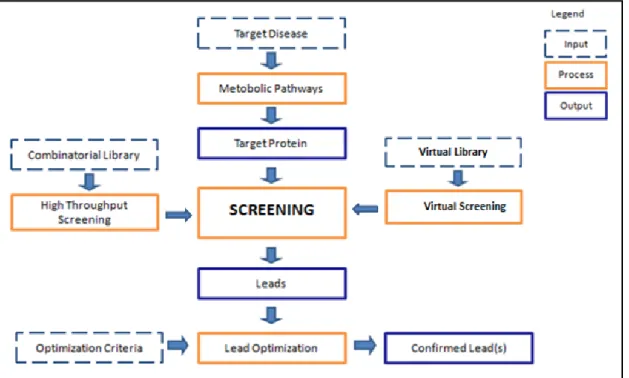
In the search of suitable drug candidates, a large numbers of compounds are evaluated in order to find molecules that are effective against the biological target. This screening process is known as high throughput screening (HTS), which is an approach to target validation. It allows the assaying of very large numbers of potential compounds against a chosen set of defined targets using an in vitro technique. This involves controlled environment and equipment. The most potent compounds obtained are called hits. HTS can rapidly select those substances that affect the target; however, it is expensive, requires extensive skills and HTS data are typically noisy or false positives. Much effort has been invested in the use of
4 computational methods to increase the speed and reduce the cost of lead discovery. The range of techniques developed for this purpose is generally referred as virtual screening (VS). VS involves the computational filtering of a large body of molecules (e.g., comprising a company‟s corporate database) to identify those that have a high probability of activity in a biological test system of interest. Thus, the VS method takes as its input all of those molecules that might be acquired (or synthesised) and tested. It then gives as its output the few molecules that should actually be tested. VS methods are increasingly being used to increase the cost-effectiveness of drug discovery programmes (Klebe, 2000).
Virtual screening is an in silico analogue of HTS which aims to identify which compound to synthesise or to purchase and to select compounds for an in vitro experiment. VS can help to analyse the results of an HTS run by identifying false positives hits. Over the past years, VS has become an essential companion of HTS as they are complementary to each other to support the lead discovery process. One popular approach to virtual screening involves the use of algorithms from the area of computer science which are referred to machine learning. A machine-learning method takes as its input a training set of compounds that have previously been classified as active or inactive. These are then analysed to develop a model that can be used to classify new molecules into active or inactive classes.
The earliest example of a machine learning method in chemoinformatics is considered to be the Substructure Analysis (SSA), while popular ones used today is Support Vector Machines (SVMs), Random Forest (RF) and Artificial Neural Networks (ANN). SSA, in particular, was proposed by Cramer in the 1970s. It was based purely on the identification of suitable lead compounds based on the relationship between molecular activity and fragment structure. SSA uses this relationship to extract a fragment weighting scheme, which is applied to the compounds for scoring, ranking and finally for assessment. The main criterion of the assessment is based on the number of active molecules that occur in the top of the ranking. The SSA method has been further developed through the introduction of various weighting schemes. It has not, however, progressed as much as other machine learning methods in recent times. SSA is very closely related to the Naïve Bayesian Classifier (NBC), a machine learning method that has become very popular in the last few years with its availability in the Pipeline Pilot system (Hert et al., 2006). NBC is a simple classification algorithm that is based on the use of Bayes‟ theorem and on strong assumptions as to the statistical independence of the descriptors characterising the objects that are to be classified. Here, it is
5 argued that the SSA is still a unique method to identify potential compounds based on its simplicity. It is a simple yet powerful method of quantifying a compound‟s influence purely on the basis of the fragment properties (via weighting schemes). As it has never been attempted before, the question remains as to whether there can be any possibility of improving the SSA method and its weighting scheme definition through the use of more robust and evolutionary approaches, specifically the GA (genetic algorithm) and GP (genetic programming). Both of these have reported success in various fields of application. The other question is whether both approaches, which are stochastic in nature, can be enhanced through the use of the use of a data fusion method. Data fusion is a deterministic method to produce a single, unified outcome.
1.3 Research aim and objectives
The aim of this study is to develop new weighting schemes in SSA that might have a better level of prediction performance than the existing procedures, based on evolutionary approaches. This application may enhance the cost-effectiveness of research programmes seeking to identify novel bioactive molecules. In order to achieve the above aim, several research objectives have been identified which need to be explored as summarised below:
i) The first research objective is to quantify the level of performance of all of the existing SSA weighting schemes, which have been introduced by various researchers, and establish the best overall scheme.
ii) The second objective is to assess the use of GA to determine the fragment weighting scheme to be used in the SSA and whether it can provide an upper-bound to the performance of the SSA when compared to the existing weighting schemes. The level of improvement will be quantified, if any uplift exists.
iii) The third objective is to investigate the use of GP to determine a fragment weighting scheme to be used in the SSA. It is thus necessary to determine whether it can provide an upper-bound to the performance of the SSA when compared to both the existing weighting schemes and the GA-based scheme. The level of improvement will be quantified, if any uplift exists.
iv) The final objective is to investigate and assess the use of data fusion, a technique that combines multiple ranking to provide further enhancement to the GA and GP-based SSA.
6 1.4 Thesis outline
This chapter describes a general introduction to the concept of chemoinformatics. This includes its application in the real world and the discussion on the virtual screening research background. This research focuses on ligand-based virtual screening, specifically on SSA. Based on the research aim and objectives defined in Section 1.3, the study is organised into eight chapters.
Chapter 2 of this thesis begins with an overview of the main elements of extracting information from a chemical structure. Commonly used methods for molecular descriptors and molecular representation are also included. Chapter 2 also reviews the basic principles and the development of the SSA method used in this thesis. Chapter 3 discusses the experimental design used in this study. It includes the details of the databases, the evaluation methods and the statistical analyses adopted to evaluate the results of the experiments conducted in this study. Chapter 4 reports on the comparison and the evaluation of the existing SSA weighting schemes. In total, ten published SSA weighting schemes are analysed. Chapter 5 investigates the use of the GA approach to weighting schemes to identify whether GA-based weighting determination yields similar or improved results when compared to the existing SSA weighting schemes. The GA approach is based on its direct determination of fragment weights as opposed to the pre-existing SSA weighting schemes. Thus, the feasibility of such a method is compared against existing weighting schemes in terms of an improvement in predictive performance. Chapter 6 examines the use of GP to develop new weighting schemes, taking as a starting point the pool of possible variables and the pool of simple arithmetic operators. The new weights resulting from the GP are then evaluated. Chapter 7 investigates the use of the data fusion method to combine the retrieval results from the multiple GA and GP searches, in which eight fusion methods are applied and assessed. Chapter 8 draws this work to a conclusion, with suggestions for more investigation into and further improvement of the SSA.
7
Chapter 2
Virtual Screening and Substructural Analysis
2.1 Introduction
The evolution of chemical computing has given rise to several established chemical information storing methods, and subsequently machine-led screening processes. Central to such methods are the extraction, analysis and manipulation of fragments from compounds. These methods are performed in silico to guide the initial discovery stage of the drug design processes. It is therefore necessary to consider potential chemical-based attributes, such as the activity and relevance of the molecules in question. Theoretically, this should increase the likelihood of discovering novel compounds for further lead verification and optimisation. This chapter describes the methods used to store and retrieve chemical structures. In addition, there are two principal components that will affect the performance of substructure analysis (SSA). These are the representation used to characterise the compounds, and the SSA weighting functions used to compare them.
2.2 Representation of chemical structures
The search for desirable compounds in existing databases is largely influenced by the clarity and accessibility of molecular information to chemists in the chemical search space. This has led to the introduction of various formats of chemical representations. Such forms of compound representations may range from simple to complex, depending on the requirements imposed on such representations. Two common forms of presentation are connection tables and line notations.
2.2.1 Connection tables
Connection tables are effective in documenting atoms and the bonds between them, which are not readily available in other types of 1D- or 2D-based structural representations. Figure 2.1 below shows an example of a connection table for the compound Aspirin. The table is primarily formed by capturing the spatial coordinates of each atom by definition of its x, y, and (perhaps) z coordinates of the atom, and their associated bonds. A connection table also provides bond information for each atom forming the compound.
8 Figure 2.1: Connection table representation (after Leach & Gillet, 2007). Information such as atom coordinates relating to its formation and bonding pairs are stored for accurate rebuilding
of the molecules
The connection table shown above is the simplest form of representation. More detailed forms may include further additional information, such as the hybridisation states of the atoms and the bond orders (Leach & Gillet, 2007). Hydrogen atoms are usually not included in the majority of standard connection tables, but this is also the case for many other structural notation systems (such as in SMILES, as will be discussed below). Information regarding the (xy) or (xyz) coordinates of the atoms enables standard chemical drawings to be produced for use in a molecular graphics program or any 3D molecular manipulation / analysis methods.
2.2.2 Morgan algorithm
The atoms of chemical compounds originally are not denoted with descriptive labels and the numbering system may be arbitrary. Issues arise when many different labels for the atoms can be represented for the same chemical compound. The Morgan algorithm can be used to solve this problem by providing a canonical label or a unique number for an atom. Canonicalisation is an important concept in chemical representation, as it allows the representation of a
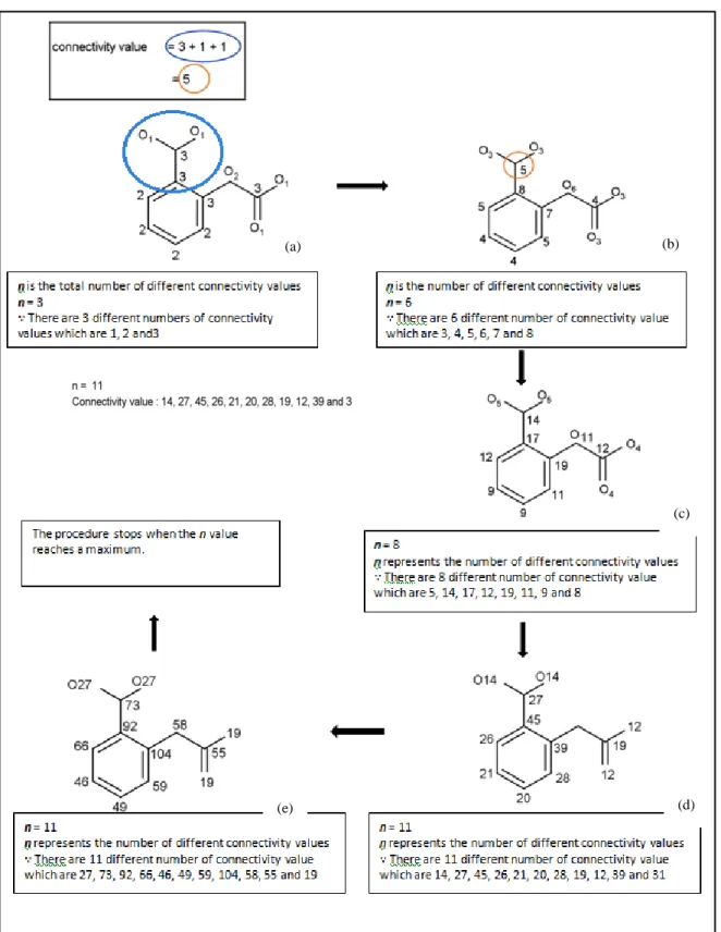
9 particular compound to be unique and unambiguous. The Morgan algorithm uses iterative calculations of the connectivity values to differentiate atoms, as illustrated in Figure 2.3.
Figure 2.2: Morgan algorithm procedure (after Leach & Gillet, 2007)
(a) (b)
(c)
(d) (e)
10 From Figure 2.3, a compound is first defined as a series of connected atoms, where the connectivity value of each atom is calculated from the number of connections to other atoms. The next iteration seeks to update the connectivity value of the atom based on the initial values of the neighbouring atoms (Figures 2.3(b) and (c)). For example, the orange highlighted atom in Figure 2.3(b) has its connectivity value updated to 5, as a summation of the connectivity values of its neighbours, which are 1, 1 and 3 respectively. The iteration continues for each atom until a maximum connectivity value is reached, as shown in Figure 2.3(e). Based on the finalised connectivity values, the connection table uses atoms with the highest connectivity value as the first atom for definition, and subsequently other atoms in decreasing order of their connectivity values (Leach & Gillet, 2007).
2.2.3 Line notation
Line notation is a compact, alphanumeric representation of molecules. It is more compressed than connection tables. It is thus able to encode a large number of molecular structures while requiring only a small memory space for storage. It is widely used for storing, representing, communicating and checking the identity of chemical structures. It can encode structures in compact form, and this may be human-readable and writable. It can also be easily used with respective software, and it also provides a canonical representation. Line notation is of particular importance in chemoinformatics which include Wiswesser Line Notation (WLN), Simplified Molecular Input Line Entry System (SMILES) and InChI (Willett, 2009). Linear notation represents the complete constitution and connectivity of chemical compounds as a linear sequence of character.
A given chemical structure can have many valid and unambiguous representations. A molecule may be presented in the form of a different numbering system for the atoms in connection table. It would be useful to use a standard numbering system to derive a single unique representation. The process of converting an input representation to a canonical form is called canonicalisation. Many methods have been developed for a unique and unambiguous numbering of the atoms of a molecule. The canonicalisation process involves deriving a canonical code for numbering or labelling the atoms in a unique and reproducible way (Gasteiger & Engel, 2006). Canonical-based representations introduced with WLN, SMILES and InChI will be discussed in greater later in this chapter.
11 2.2.4 Wiswesser Line Notation (WLN)
Wiswesser Line Notation (WLN) was developed by William Wiswesser in the 1950s. It was considered one of the most popular and widely used notations to enforce canonical representation of molecules, whereby each molecule has one and only one formula. Figure 2.2 below stresses the exclusive relationship between the computer representation and the molecular structure. „Unique’ refers to only one instance of computer representation derived from a structure; „Unambiguous‟ refers to only one structure produced from one computer representation.
Figure 2.3: Canonical state of structure for computer representation (adapted from UTM open courseware chemistry website)
WLN represents structural formulae with a short combination of numerals, capital letters and punctuation marks. It also makes extensive use of special symbols to denote common structural fragments. These symbols are formed into a specific code by encoding them in the same order in which the fragments are connected in the structural formula (Vollmer, 1983). A set of rules is devised to ensure that such notations enforce a canonical form, as shown in Figure 2.2. Although WLN has been widely used to represent structures in the form of line notation, it was difficult to adopt and maintain. This is mainly because many rules must be followed to generate the correct notation of a complex structure (Weininger, 1988). It thus proved particularly difficult to implement notation in computer terms; consequently, this led to the introduction of alternative notation systems instead.
2.2.5 Simplified Molecular Input Line Entry System (SMILES)
SMILES is one of the most popular line notations in current use. It was created in response to the need for a simpler, more computer accessible and human-friendly notation than WLN. SMILES retains the concept of canonical representation, but it is easier to encode with a computer than was the case with WLN. The original SMILES specification was developed by Arthur Weininger and David Weininger in the late 1980s. It has since been modified and extended by numerous other organisations (Weininger, 1988).
12 In 2007, an open standard called OpenSMILES was developed by the Blue Obelisk open source chemistry community (http://www.opensmiles.org). In SMILES, atoms are represented using their respective atomic symbol. Upper case letters refer to aliphatic atoms; lower case letters refer to aromatic atoms. If the atomic symbol has more than one letter, the second letter must be in lower case. The structures entered using SMILES are hydrogen-suppressed, which means that the molecules are represented without hydrogen atoms. SMILES is able to handle branches denoted with the symbol ( ) and also supports nesting. In terms of bonding, the following is used: „-‟ for a single bond (which are usually not shown at all); „=‟ for double bonds; „#‟ for triple bonds and „:‟ for aromatic bonds. Single and aromatic bonds may always be omitted. Many weak points of other line notation systems can be attributed to the overuse of symbols and hierarchical rules based on the length of the final notation. SMILES notation was designed to introduce a standard, unified description of chemical structures so that it can be used and understood by both users and computers. For example, a chemist is able to retrieve a list of compounds from a database defined in terms of coded strings as notated by the SMILES. The selected compounds in SMILES notation can be further utilised with a computer to identify structural descriptors as necessary. Likewise, chemical information can be exchanged universally with ease between researchers by utilising the standard unique SMILES string to name a molecule. Chemical programmers also use SMILES in the process of entering chemical data into a computerised database, and thus, maintaining unique structural descriptions is necessary. The description used by computers requires a far more complex set of rules and hierarchies, and this translates to an extensive dependency on an efficient computer algorithm (Weininger, 1988).
2.2.6 International Chemical Identifier (InChI)
InChI is a recent notation system introduced to standardise chemical structure information. InChI was a joint project by many organisations, such as standards agencies, chemical field experts, and educational and commercial based participants. The goal was to achieve a more consistent and standardised definition of chemical structures. InChI uses a layered format to represent all the available structural information relevant to compound identity, where by each layer designates a specific type of structural information, with the layers ordered to provide successive structural refinement. There are six major InChI layer types, with each giving a different class providing structural information. The InChI layers consist of the main layer, a charge layer, a stereochemical layer, an isotopic layer, a fixed-H layer and a reconnected layer. The main layer, which specifies chemical formula, atoms, and bonds between them, is
13 required for all InChIs. However, the other layers appear only when corresponding input information is provided (Heller, McNaught, Stein, Tchekhovskoi & Pletnev, 2013). Every InChI starts with the string "InChI=" followed by the version number, currently 1. This is followed by the letter S for standard InChIs. Layers and sub-layers start with “/” (forward slash) followed by a letter denoting the identity of the layer (except for the chemical formula layer). InChI notations are meant to be processed and decoded by computers only: they are not designed to be interpreted by users. Comparisons between SMILES and InChI have been drawn in various studies (Boda, 2010), where the former has more flexibility and the latter is more consistent in terms of representations. SMILES is proprietary and has more software support. As O‟Boyle (2012) states: “other commercial and open-source software developed their own algorithms for generating canonical SMILES all of which differed from each other and none of which are published” (O‟Boyle). This has led to the use of different generation algorithms, and thus, different SMILES versions of the same compound have been found. The lack of a single commonly-adopted standard has resulted in inconsistent representation terms. To address the lack of a non-proprietary, strictly-unique standard chemical identifier, the InChI project was initiated. InChI is non-proprietary, open-source, and freely available to the scientific community. As the software for generating InChI strings is freely available, it also avoids the interoperability issue. SMILES, however, is generally considered to be more human-readable than InChI. Table 2.1 shows the comparison between the SMILES and InChI notations.
14 Table 2.1: Linear chemical notation
Bonds IUPAC Name Chemical Compound Chemical Formula SMILES IUPAC Standard InChi Single Bond Ethane C2H6 CC InChI=1S/C2H 6/c1-2/h1-2H3 Double Bond Ethene H2C=CH2 C=C InChI=1/C2H4/ c1-2/h1-2H2 Triple Bond Hydrogen Cyanide HCN C#N InChI=1S/CHN /c1-2/h1H Aromatic Bond Dimethyl Ether
CH3OCH3 COC InChI=1S/C2H
6O/c1-3-2/h1-2H3
Branches Triethylamine N(CH2CH3)3 CCN(CC)CC InChI=1S/C6H
15N/c1-4-7(5- 2)6-3/h4-6H2,1-3H3
2.3 Molecular descriptors
The manipulation and analysis of chemical structural information often requires the use of molecular descriptors generated from the molecule representations described above. The molecular descriptor can characterise and classify structural patterns by means of encoding, using numerical values to characterise the properties, e.g. the physicochemical properties of molecules (Todeschini & Consonni, 2008). A descriptor classification essentially requires two criteria: the molecular representation of the compound, and the algorithm used to calculate the descriptor information. These descriptors may contain detailed information regarding various properties useful for analysis within Virtual Screening, such as the Structure-Activity-Relationship (SAR), Quantitative-SAR (QSAR) studies and molecular diversity analysis. It is reported that there are more than 3,000 different types of molecular descriptors available (Leszczynski & Shukla, 2009). For any typical drug discovery process, however, only descriptors that successfully correlate structural features with the biological activity of interest are explored (Khanna & Ranganathan, 2011).
There are several ways to classify descriptors, categorised as physicochemical (hydrophobic, steric or electronic), structural (frequency of occurrence of a substructure), topological,
15 electronic (molecular orbital calculation) or geometric (molecular surface area calculation). Molecular descriptors (specifically, physicochemical descriptors) can also be categorised into two groups. The first is the descriptors representing properties of molecules, for instance, the logP and the molecular weight. Physicochemical parameters govern the physical and chemical properties of chemical entities. The behaviour of bioactive chemical entities may be affected by changes in physicochemical properties. Physicochemical properties are also known as an example of 1D descriptors. Examples of properties include molecular weight; logP (the logarithm of the partition coefficient between octanol and water) which quantifies a molecular hydrophobicity, solubility and simple count of features (e.g. number of atoms, H-bond donors, H-bond acceptors and ring systems). All these properties can be used as part of QSAR studies, which correlates quantitative chemical structure attributes (e.g. physicochemical, biological and toxicological) of molecular descriptors to a biological activity. For instance, Lipinski et al. (2012) in their studies of solubility and permeability prediction in drug discovery used four physicochemical properties. These were molecular weight, sum of nitrogen, oxygen and hydrogen-bond acceptors.
The second type is descriptors categorised according to dimensionality, which are 2D, and 3D. 2D descriptors are derived from molecular connectivity table and apply a simple count of features to characterise molecules. Examples of 2D descriptors calculated from 2D graphs are topological indexes and 2D fingerprints.
3D descriptors are generated from 3D connection tables, which can be obtained either experimentally or theoretically. For example, a 3D structure builder such as CONCORD or CORINA (Clark, 1999) can generate 3D structures from the chemical graph. Examples of descriptors requiring 3D representations are the pharmacophore descriptors, affinity fingerprints, distance-based descriptor, 3D atom environment for use in atom mapping similarity searching and 3D molecular fields for use in field-based similarity searching. 3D molecular field descriptors involve generally a 3D grid, each element of which is characterised by the values/properties of the steric, electrostatic and hydrophobic. It should be noted that these 3D properties are used in QSAR methods, such as Comparative Molecular Field Analysis (COMFA), where it is one of the most significant development in QSAR. This research, however, focuses only on 2D descriptors, which are considered more appropriate to the aims of this research, namely, the SSA. There are also several descriptors, which are based