Financial constraints and the balance sheet channel: a re-interpretation

FINANCIAL CONSTRAINTS AND THE

BALANCE SHEET CHANNEL

: A

RE-INTERPRETATION

Marco Gallegati

*

Dipartimento di Economia, Università di Ancona, Piazzale Martelli 8, 60121 Ancona, e-mail: [email protected]

Abstract. Aggregate demand models extending IS/LM fixed price framework yield an enhancement mechanism of the traditional monetary transmission mechanism, the credit channel, which, according to the credit view, works through the ‘balance sheet channel’ and the ‘bank lending channel’. In this paper I modify the augmented IS/LM model assuming that investments may be financed by both internal and external sources of funds. The inclusion of internal funds in the augmented IS/LM fixed price model suggests a different interpretation of the ‘balance sheet channel’ as an enhancement mechanism amplifying monetary policy effects through the quantity rather than the cost of borrowing. Thus, changes in borrowers’ net worth over the cycle can amplify and propagate output fluctuations directly rather than indirectly as in the traditional interpretation of the balance sheet channel. The empirical analysis of the monetary transmission mechanism for Italy in the last decade accords with the interpretation of the balance sheet channel proposed in this paper.

Keywords: Financing Constraints, Credit View, Balance Sheet Channel, Impulse Response Analysis.

JEL: E51, G32

* _{I wish to thank Marco Crivellini, Giuseppe Marotta and Marco Mazzoli for their comments} and suggestions to an earlier version of the paper. This paper is part of MURST’s research program “Heterogeneity in bank and trade credit markets and in local financial systems: implications for regional growth and distributional effects of monetary policy”. Financial support from MURST is gratefully aknowledged. The usual disclaimers apply.

1. Introduction

For many years economists, under the assumption of perfect capital markets, ignored the role of credit market in determining real economic activity. The recent literature examining the consequences of asymmetric information in financial markets stresses that, contrary to the financial irrelevance proposition of the Modigliani-Miller theorem, financial conditions matters for investment decisions (Messori, 1996, Stiglitz, 1988, 2000). Indeed, as capital market imperfections make external funds available at a higher cost than the internal ones, a financing hierarchy is likely to emerge and firms may be financially constrained in their investment decisions, i.e. they may postpone or forsake positive net present value investment projects (Kaplan and Zingales, 1995).

Empirical works, both at aggregate and individual level, tend to confirm the influence of financial factors on corporate investment decisions in many countries. Several studies considering aggregate corporate financing patterns find some regularities, both at single country level and in international comparisons, indicating that retentions are the dominant source of fund and that bank loans are the main source of external finance (Mayer, 1988, 1990, Mac-Kie Mason, 1990, and Taggart Jr. 1990). Moreover, empirical estimates of investments equation using q models find that the inclusion of cash-flow variables significantly improves the performance of investments equation (Fazzari et al., 1988, Bond and Meghir, 1994, Hoshi et al., 1991, among the others).

Aggregate demand models extending IS/LM fixed price framework (Brunner and Meltzer, 1968, 1972, Bernanke and Blinder, 1988, 1992, Dale and Haldane, 1993a, 1993b) relax the assumption of perfect substitutability between bank and non-bank sources of credit, both as banks' assets and as non-bank private sector's liabilities, providing an explicit role for the supply side of the credit market. These modification of the original framework yield an enhancement mechanism of the traditional monetary transmission mechanism, the credit channel, which, according to the credit view, works through the balance sheet channel and the bank lending channel. In the credit view of the monetary transmission mechanism the first channel stresses the impact of monetary policy on borrowers’ financial position (net worth, cash flow and liquid assets) on the size of the external finance premium and then on investment spending, while the latter stresses the possibility that monetary policy may affect the supply of intermediated credit, particularly bank loans.

In this paper I modify the augmented IS/LM model assuming that investments may be financed by both internal and external sources of funds. The inclusion of internal funds in the augmented IS/LM fixed price model suggests a different interpretation of the balance sheet channel as an enhancement mechanism which amplify interest rates effects working through the quantity rather than the cost of borrowing. In this sense, borrowers’ availability of internally generated funds which

may be directly used for financing investment projects may give rise to a higher monetary policy effectiveness as the result of the reduction of the financial constraints on firms’ investment behaviour. Moreover, with this interpretation of the

balance sheet channel, movements in borrowers’ balance sheet will amplify and propagate business cycles fluctuations directly and not indirectly, as usually stated by the ‘financial accelerator’ effect working through banks’ behaviour. Such an interpretation of the balance sheet channel seems more in line with the common practice in banking relationship with firms, where price discrimination depends on parameters like the existence of a long or short term relationship, firm’s size and/or firm’s business volume with the bank.

2. The model (an augmented IS/LM fixed price model

with internal funds)

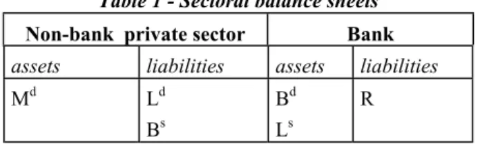
The augmented IS/LM framework is defined over four markets, goods, money, credit and bonds, and two sectors, the non-bank private sector (nbps from now on) and commercial banks. The public sector is absent in this model as bonds are issued by the nbps and not by government. The balance-sheets of the two sectors are represented in Table 1. The nbps’ liabilities comprise their borrowings from the banking sector, Ld, and their net issue of bonds, Bs, which are balanced by their money holdings, Md. The banking sector supplies loans to nbps, Ls, and invests in bonds supplied by the nbps, Bd, the reserves borrowed from the central bank, R.

Table 1 - Sectoral balance sheets Non-bank private sector Bank

assets liabilities assets liabilities

Md Ld Bs Bd Ls R Credit market

Looking at sectoral balance sheets we note that the supply side of the credit market (loan supply) represents a bank asset, while its demand side (demand for bank loans) is a liability of the non-bank private sector. Banks' choice of asset composition between loans and bonds depends on portfolio considerations. Banks' loan supply depends positively on the interest rate on bank loans and negatively on the interest rate on bonds. Moreover, it depends positively on the level of reserves,

Ls= Ls

(

i,ρ, R

)

(1) where L_is<0, Ls_ρ >0 , Ls_R>0.

On the other side firms' demand for investment gives the demand for bank loans. Investment demand is assumed to depend on both the cost of capital, negatively, and aggregate output, positively, as in the standard flexible accelerator model (Jorgenson, 1963). The nbps' demand for bank loans depends on considerations involving firms' investment and financing decisions. If the firm's optimal investment level is I, it may choose to finance it using retained earnings at the opportunity cost

δ,1 bank loans at the interest rate ρ, and new bonds issue at the interest rate i. The relationship between firm's investment spending and its sources of funds is given by the following identity:

I= IF+Ld+Bs (2)

where IF is the amount of internally generated funds available for investment spending. These funds are residual in nature, as they represent what remains to the firm after paying wages, w, and dividends, d. Given the fixed price framework of the augmented IS/LM framework and assuming the constancy of dividends through the time2, we may express retained earnings, IF, as

IF = (1-a) y (3)

where a is (w + d) / y. Thus, if we consider equation (2) may be written as

I−

(

1−a

)

y= IN =Ld+Bs (4) where IN _{represents investments out of retained earnings, that is firm's external} financing needs.

Assuming, as in Kashyap et al. (1993), that firms need external funds, each firm will choose to finance a fraction α of investment IN _{with bank loans and a fraction} (1-α) issuing bonds, and being α* firm's optimal financing mix between bank loans and bonds, the cost of capital for a firm will be given by a weighted sum of the cost of both external sources of funds (if we assume a cost opportunity for internal funds equal to zero):

k=

( )

1−α* i+α*ρ=i+

(

ρ−i

)

α* (5)

1 _{Given the absence of government bonds we set the opportunity cost of retained earnings} equal to zero.

where α*=Ld

IN =α

(

i−ρ

)

is firm's optimal financing mix (with

1−α*

( )

=Bs IN ).

Firm's investment demand, as in the standard flexible accelerator model, (Jorgenson, 1963), is assumed to depend positively on aggregate output and negatively on the cost of capital

I= Id

( )

y,k (6)

so that investment demand out of retained earnings is

IN =Id

( )

y, k −

(

1−a

)

y (7) From the definition of α* and IN we may derive the demand for bank loans Ld as

Ld₌α*IN ₌ Ld

(

i,ρ, y

)

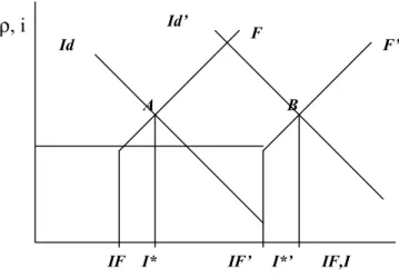
(8) where loan demand depends, via α*, negatively upon its own rate, ρ, and positively on the bond rate, i, i.e L_id>0, L_ρd <0 . Moreover, as a change in aggregate income affects both investments demand and retained earnings in the same direction, the derivative of the demand for loans with respect to income, Ldy, will be lower or equal to the one which characterises the augmented IS/LM model without internal funds. In particular, it will be lower if the effect of a change in aggregate income on the level of retained earnings will be positive; it will be equal if the effect of this change will be zero.

Figure 1 –Effect of an increase of income on the demand for loans

Id

Id’

F

F’

IF I* IF’ I*’ IF,I

ρ

, i

The effects of an increase in income on the demand for loans are presented in figure 1. The demand for loans is measured on the horizontal axis by the difference between I* and IF (the figure refers to the case in which debt is the only external source of funds). An increase in income cause a shift to the right both of the Id curve and of the F curve, so that the final effect on the demand for loans may not be determined a priori as it will depend on the relative movements of the two curves. Anyway, the inclusion of internal funds among the sources available to firms in financing investments let the derivative of the demand for loans with respect to income, Ld_y, assume a lower (at limit even negative) value as regards the conventional augmented IS/LM model.

Money market

Absent nbps’ cash holdings, deposits equal money supply, Dd =Ms, and reserves equal monetary base, R=B. Then, we define the money supply function with the usual money multiplier relationship:

Ms= mR (9)

with m>0.

Given the nbps' balance sheet condition shown in table 1 the specification of the

nbps’ demand for money needs some explanations. Absent government bonds, nbps’ opportunity cost of money holdings is represented by the cost of borrowing from the banking sector, either via bank loans or via bank holdings of the bonds they issue. The higher the cost of borrowing, the greater will be the cost of money holdings. Thus, the nbps’ demand for money will depend inversely both on the interest rate on loans and bonds. Finally, as usual, money demand depends positively on income due to the transactions motive:

Md =Md

(

Y, i,ρ

)

(10) with M_yd >0, M_id >0 and M_ρd >0.

Goods market

Aggregate demand equals investment demand, and given the assumption of a horizontal aggregate supply curve, the nbps' demand for goods determines goods market equilibrium. The investment demand function (6) implies that aggregate income depends negatively both on the interest rate on loans and on the interest rate on bonds:

with Iy>0,Ii<0 and Iρ <0.

Bond (Equity) residual market

By Walras' law equilibrium in the bond market is derived, residually, from the equilibrium of the other equations in the model.

3. Comparative statics results of a monetary policy

shock

The general equilibrium of the model is solved for the seven endogenous variables

(

Y ,i,ρ,α, k, Id, IN

)

by imposing output, money and credit market equilibrium together with the condition that the banks’ balance-sheets constraint is satisfied. Total differentiation of the equilibrium condition for the goods, money and credit markets gives the following system:

1−I_y −I_i −I_ρ M_yd M_id M_ρd L_yd L_id−L_is L_ρd −L_ρs           ∂y ∂i ∂ρ           = 0 m Ls_R           ∂ R

[ ]

(12)

Let's look at the comparative static results of a monetary policy shock. An expansionary (contractionary) monetary policy will increase (decrease) the level of income, that is ∂Y_∂R>0

(

∂Y_∂R<0

)

, ''for plausible parameter values'' (Dale and Haldane, 1993a): ∂Y ∂R= mY_ρ

(

L_id−L_is

)

+mYi

(

Lρd−Lsρ

)

+LsR

(

YiMid−YρMid

)

1−I_y

( )

M_ρd

(

L_id−L_is

)

+

( )

1−I_y M_id

(

L_ρs −Ld_ρ

)

+M_ydY_ρ

(

Ld_i −Ls_i

)

+M_ydY_i

(

Ls_ρ−L_ρd

)

+Ld_y

(

Y_iM_ρd−Y_ρM_id

)

(13)

The transmission mechanism underlying this comparative static result works as follows: the increase (decrease) in reserves let the banking sector increase (decrease) both the supply of loans and the demand of bonds. Both interest rates will fall (rise) as a consequence of the increased (reduced) banks’ demand for bonds and supply of loans. This, in turn, stimulates, through the investment function, an increase (decrease) in the equilibrium level of income which restore, through the fall in the bank and bond rate, the equilibrium in the money market. Under the conventional augmented IS/LM model (Bernanke and Blinder, 1988, Dale and Haldane, 1993a) the expansionary (contractionary) impact of monetary policy will be partially offset

by the increased (reduced) nbps’ demand for loans following the increased (reduced) level of income. As a consequence, these second round effects lowers the impact of a monetary policy shock on income through the fall in the bank loan rate.

From the augmented IS/LM model with internal funds presented in the previous section we know that, as the increase in investment demand following an increase in income will give no more place to a one to one increase in the demand for external funds as part of the new investments will be financed by internally generated funds, the magnitude of Ld_y will be lower than that of the conventional augmented IS/LM model. Thus, when we include the possibility of using internally generated funds in financing investments, the offsetting second round effects lowering monetary policy effectiveness will be tempered by the limited reduction of the bank loan rate due to the reduced magnitude of Ld_y. The way Ld_y affects bank loan rate may be determined looking at the responses of the bank loan rates to a monetary shock:

∂ρ ∂R= m _

( )

1−Iy

(

L_id−L_is

)

+LdyIi _{ −}Ls_R

[

( )

1−Iy M_id +IiMyd

]

1−Iy

( )

M_ρd

(

L_id−Ls_i

)

+

( )

1−Iy Mid

(

Lsρ−Lρd

)

+MydYρ

(

Ldi −Lis

)

+MydYi

(

Lρs −Ldρ

)

+Lyd

(

YiMρd−YρMid

)

(14)

Equation (14) shows that, as pointed out in Bagliano and Favero (1994), a small effect of aggregate demand on the demand for banks’ loans is required even in order to have the bank loan rate moving in the opposite direction as the change in reserves.3 And given that the inclusion of internally generated funds reduces the magnitude of Ld_y, the final change in the bank loan rate will be higher the lower will be the magnitude of Ld_y. In this way, monetary policy effectiveness will be higher in the augmented IS/LM model with internal funds with respect to the standard augment IS/LM model.

“Credit view” explanations of the magnitude of the economy’s response to monetary policy shocks stress the effects of a policy change on the external finance premium through the balance sheet and the bank lending channels (Bernanke and Gertler, 1995). According to the “credit view”, the balance sheet channel stresses the additional effects of monetary policy changes on interest rates through the changes in borrowers’ balance sheets variables like net worth, cash flow and liquid asset, affecting the size of the external finance premium. On the contrary, in our model the balance sheet channel represents an enhancement mechanism which amplify interest rates effects affecting the quantity rather than the cost of borrowing. Indeed, the

3 _{A sufficiently small elasticities of loan demand to the level of goods demand is even} necessary in the model of Bernanke and Blinder (1988) in order to have the interest rates moving in the same direction after a monetary policy impulse.

effects on the interest rates go from quantities to prices and not vice versa. Changes in borrowers’ net worth determined from the first round effects of an expansionary (contractionary) monetary policy, reduce (increase) the need for external finance and the second round effects on the cost of external finance. We may interpret this higher monetary policy effectiveness as the result of the reduction of the financial constraints on firms’ investment behaviour, being liquidity constraints linked to the availability of internally generated funds. Thus, changes in borrowers’ net worth over the cycle can amplify and propagate fluctuations in output, a business cycle propagation mechanism referred as the “financial accelerator” (Gertler, 1994). These sort of results resembles the ones of those macroeconomic models of the New Keynesian Economics which highlight the role of internal funds for the level of economic activity. Indeed, both Bernanke and Gertler (1989) and Greenwald and Stiglitz (1990) present models where an accelerator effect emerges as firms’ financial conditions over the cycle contribute to amplify output fluctuations.

4. Evidence from Vector AutoRegression

In this section we try to verify the interpretation suggested in the previous section about the way the balance sheet channel may works inside the monetary transmission mechanism examining the effects of monetary policy. Given the lack of consensus about a complete structural model of the economy, has become common practice to analyze the effects of monetary policy using Vector AutoRegressions (Bernanke and Blinder, 1992, Sims, 1992, Dale and Haldane, 1993b, Gertler and Gilchrist, 1993, Bernanke and Gertler, 1995, Christiano et al. 1996, and Bagliano and Favero, 1994). Indeed, as the Vector AutoRegressions (VARs) is a system of linear equations, one for each variable, where each endogenous variable in the system is a function of all of the endogenous variables in the system, it avoids the problem of specifying a complete structural model of the economy. Moreover, once estimated, it may represents a convenient way to simulate the dynamic effects of monetary policy actions on the behaviuor of the economy.

Testing for cointegration

In order to provide some econometric evidence on the transmission mechanism of monetary policy we estimate a VAR model which, following the specification of the theoretical model of the previous section, includes a monetary policy instrument (the monetary base), financial variables (bank loans and the interest rate on bank loans), and a final policy objective (the index of industrial production). The sources of the data set are the Bank of Italy’s Economic Bullettin for total monetary base, total bank loans and the average interest rate on bank loans, and the Istat’s Monthly

Bulletin of Statistics for the seasonally adjusted index of industrial production (base year=1990). All variable but the interest rate on loans are expressed in logharitms, and both total monetary base and total bank loans are expressed in real terms after deflation by the consumers' price index. The data are taken at a monthly frequence over the period 1993:2-2001:3. Earlier observations are excluded because of the high instability characterizing the last quarter of 1992 which culminated in the exit of Italy from the EMS.

Preliminary application of unit root tests to the four variables included in the VAR shows that each variable appears to be non-stationary. With four non-stationary variables there may be from zero to three (long-run equilibrium) cointegrating relationships among them. In order to test for the existence of cointegrated vectors among the included variables we apply the methodology developed by Johansen (1988, 1996) which tests the restrictions imposed by cointegration on the unresctricted VAR expressed in the following form:4

∆∆∆∆yt=c+µDUt+ ΓΓΓΓi i=1

3

∑ ∆∆∆∆yt−1+ΠΠΠΠyt−2+εt (16) where DUt is a step-dummy variable5 and Π=αβ’ is a 4x4 matrix with α and β being two 4xr matrices of the speed of adjustment and cointegrating parameters, respectively. The number of cointegrating relations (i.e. the cointegrating rank, r) is obtained estimating the matrix Π in an unrestricted form, and then testing sequentially from r=0 to r=3 until we fail to reject the restrictions implied by the reduced rank of Π.

Table 2 - Cointegration-rank test

Trace Johansen 5% Inoue 5% Hypothesized Eigenvalue statistics asymptotic c.v. asymptotic c.v. No. of CE(s)

0.536970 122.1856 62.61 65.69 None * 0.230740 46.72907 42.20 44.52 At most 1 * 0.157134 21.02116 25.47 26.98 At most 2 0.042620 4.268377 12.39 9.53 At most 3

4 _{The optimal lag lenght of the VAR was derived using a sequence of (likelihood ratio)} exclusions tests.

5 _{The introduction of a step-dummy variable from 1998 on is required to have well-behaved} residuals as the real monetary base series has a level shift after the decisions of the Bank of Italy to reduce for three times in the same year both the minimum legal reserve requirements and its remuneration.

* denotes rejection of the hypothesis at the 5% significance level (the asymptotic critical values allowing for a model like (16) are reported in Johansen, 1996, table 15.4, and Inoue, 1999, table 1).

The results of the Johansen cointegration trace test procedure assuming for an intercept term in the cointegrating equations and no linear trend in the non-stationary part of the process are reported in table 2. They show that both the hypothesis of the existence of at most one cointegrating vector is rejected by the data, whilst that of at most two cointegrating vectors cannot be rejected by the data. Thus, the matrix Π is of rank 2 (the cointegrating rank), as 2 is the number of cointegrating relations. Thus, we estimate a three lags Vector Error Correction (VEC) model which includes, following the results of the cointegration rank test, two cointegrating equations. From the estimated VEC model we calculate the implied impulse response functions to a shock to the monetary indicator. As our primary interest is in analysing the behaviour of the economy after a monetary policy shock, we do not report the results of the VEC coefficient estimates and analyse the estimated dynamic response of the other variables with respect to an innovation in the monetary base equation residual. Impulse response analysis

VAR analysis of the effects of monetary policy, carried on through the impulse response function, requires the choice of an identification scheme in order that each reduced-form disturbance be uniquely associated with a structural disturbance. We adopt the most common type of identification scheme used in the monetary VARs, the Choleski decomposition, which implies a contemporaneous, recursive form on the system and is consistent with a Wold causal ordering.

Following the specification of the theoretical model of the previous section, the monetary transmission mechanism within our system is defined over a monetary policy instrument (monetary base), financial variables (bank loans and the interest rate on bank loans), and a final policy objective (the index of industrial production). In this way, the ordering of the variables in the VAR system will be the following: monetary base, bank loans, interest rate on bank loans and output. The placement of real monetary base at the top of a recursively ordered system requires satisfaction of the weak exogeneity assumption of the monetary policy actions. A crucial element to consider VAR monetary base equation residuals as representative of a monetary policy shock is the assumption that endogenous monetary policy actions may be distinguished from exogenous ones, as the first should be representative of the monetary authority's reaction function while the latter should consist of all other actions (Rudebush, 1998). The weak exogeneity assumption should be satisfied with monthly data as policy actions within the month should not be affected by the realised values of non-policy variables for that month.

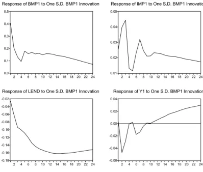
Figure 2 displays the response functions of each of the four variables (real monetary base, real bank loans, interest rate on bank loans and output) with respect to an innovation in the real monetary base residual. The qualitative patterns exhibited by the impulse response functions exhibited of the four variables of the system accords with the interpretation of the monetary transmission mechanism proposed in section 3. Indeed, following a monetary easing bank loans raise almost immediately (the first peak after about three months) while, correspondingly, the interest rate on bank loans begins to fall (reaching its minimum after about eight periods). The fall of the interest rate on bank loans stimulates output which after about eight months from the monetary policy shock begins to rise. In the medium run (12-24 months) the monetary policy shock seems to have a permanent effect on output, bank loans tends to return slowly to their original values and the interest rate on bank loans shows no tendency to return to its initial value (an effect which may be explained by the indirect effect of the balance sheet channel on the cost of borrowing). These medium run patterns of the financial variables is just what we should expect when a ''financial accelerator'' mechanism is at work. Indeed, with informational problems in external capital markets determining firms' financial constraints, the increased availability of internally generated funds will induce firms to substitute the source of funds, bank loans, with the lower one, internal funds.

Figure 2 - Impulse response functions to a real monetary base shock

0.0 0.1 0.2 0.3 0.4 0.5 2 4 6 8 10 12 14 16 18 20 22 24

Response of BMP1 to One S.D. BMP1 Innovation

0.01 0.02 0.03 0.04 0.05 2 4 6 8 10 12 14 16 18 20 22 24

Response of IMP1 to One S.D. BMP1 Innovation

-0.18 -0.16 -0.14 -0.12 -0.10 -0.08 -0.06 -0.04 -0.02 2 4 6 8 10 12 14 16 18 20 22 24

Response of LEND to One S.D. BMP1 Innovation

-0.06 -0.04 -0.02 0.00 0.02 0.04 2 4 6 8 10 12 14 16 18 20 22 24

Conclusions

The link between borrowers’ balance sheet position and investments may help explaining empirical findings6 about monetary policy ability to affect real output, at least in the short run, through the balance sheet(net worth) channel. According to the “credit view” monetary policy actions may affect the wedge between the cost of funds raised externally and the opportunity cost of internal funds, that is the external finance premium, through its influence on borrowers’ financial position.

When including firms’ internal funds as a source of financing new investments in an augmented IS/LM model, monetary policy may become more powerful since it operates directly through its influence on firms’ financial constraints. In particular, the economy’s response to monetary policy shocks is magnified by a balance sheet channel which affects firms’ investment spending decisions through the quantity rather than the cost of borrowing. Thus, changes in borrowers’ net worth over the cycle can amplify and propagate output fluctuations directly rather than indirectly as in the traditional interpretation of the balance sheet channel.

The empirical analysis of the moneatry transmission mechanism for Italy in the last decade accords with the interpretation of the balance sheet channel proposed in this paper as an enhancement mechanism amplifying the effects of monetary policy actions through the quantity rather than the cost of borrowing.

References

Bagliano F.C. and C.A. Favero, 1994, “The Credit View and a Model of the Monetary Transmission Mechanism. The Case of Italy”, mimeo.

Bernanke B.S.and A.S. Blinder, 1988, “Credit, Money and Aggregate Demand”, American Economic Review, Papers and Proceedings, 435-39.

Bernanke B.S.and A.S. Blinder, 1992, “Federal Funds Rate and the Channels of Monetary Transmission”, American Economic Review, 82, 901-21.

Bernanke B. e M. Gertler 1989, “Agency Costs, Net Worth, and Business Fluctuations”, American Economic Review, 79, 14-31.

Bernanke B. e M. Gertler, 1995, “Inside the Black Box: The Credit Channel of Monetary Policy Transmission”, Journal of Economic Perspectives, 9, 27-48.

6 _{Romer and Romer (1989), Bernanke and Blinder (1992) and Christiano et al. (1994) recent} findings show that monetary policy actions are followed by movements in real output lasting for two years or more.

Bond S. and C. Meghir, 1994, “Dynamic Investment Models and the Firms’ Financial Policy”, Review of Economic Studies, 197-221.

Brunner K. and A.H. Meltzer, 1968, “Liquidity Traps for Money, Bank Credit, and Interest Rates”, Journal of Political Economy, 76, 1-37.

Brunner K. and A.H. Meltzer, 1972, “Money, Debt and Economic Activity”, Journal of Political Economy, 80, 951-77.

Christiano L., Eichenbaum M. and C. Evans, 1996, “The Effects of Monetary Policy Shocks: Evidence form the Flow of Funds”, Review of Economic and Statistics,78, 16-34.

Dale S. and A.G. Haldane, 1993a, “A Simple Model of Money, Credit and Aggregate Demand”, Bank of England,Working Paper Series no.7

Dale S. and A.G. Haldane, 1993b, “Interest Rate Control in a Model of Monetary Policy”, Bank of England, Working Paper Series no.17.

Fazzari S., Hubbard G. and B. Petersen (1988), “Financing Constraints and Corporate Investments”, Brooking Papers on Economic Activity, 1, 141-206.

Gertler M., 1994, “Financial Conditions and Macroeconomic Behaviour”, NBER Reporter, Summer, 10-14.

Gertler M. and S. Gilchrist, 1993, “The Role of Credit Market Imperfections in the Monetary Transmission Mechanism: Arguments and Evidence”, Journal of Scandinavian Economics, 95, 43-64.

Greenwald B. and J.E. Stiglitz (1990), “Macroeconomic Models with Equity and Credit Rationing”, in Asymmetric Information, Corporate Finance and Investment, a cura di R.G. Hubbard, The University of Chicago Press, Chicago.

Hoshi T., Kashyap A. and D. Scharfstein, 1991, “Corporate Structure, Liquidity, and Investment: Evidence from Japanese Industrial Group”, Quarterly Journal of Economics, 106, 33-60.

Inoue A., “Tests of Cointegrating Rank with a Trend-Break”, Journal of Econometrics, 90, 215-237.

Johansen S., 1988, “Statistical Analysis of Cointegration Vectors”, Journal of Economic Dynamics and Control, 12, 231-254.

Johansen S., 1996, Likelihood-based Inference in Cointegrated Vector Autoregressive Models, Oxford University Press, Oxford.

Jorgenson D.W., 1963, “Capital Theory and Investment Behaviour”, American Economic Review, Papers and Proceedings, 53, 247-59.

Kaplan S.N. and L. Zingales, 1995, “Do Financing Constraints Explain Why Investment Is Correlated with Cash Flow?”, NBER Working Paper no.5267.

Kashyap A.K., J.C. Stein and D.W. Wilcox, 1993, “Monetary Policy and Credit Conditions: Evidence from the Composition of External Finance”, The American Economic Review, 83, 78-98.

MacKie-Mason, 1990, “”, in Friedman B.M. eds., Corporate Capital Structures in the United States, The University of Chicago Press, Chicago.

Mayer C.P. (1988), “New Issues in Corporate Finance”, European Economic Review, 32, 1167-89.

Mayer C.P. (1990), “Financial Systems, Corporate Finance, and Economic Development”, in Asymmetric Information, Corporate Finance and Investment, a cura di R.G. Hubbard, The University of Chicago Press, Chicago.

Myers S., 1984, “The Capital Structure Puzzle”, The Journal of Finance, 39, 575-592. Messori M.(1996), (eds.), Liquidity Constraints and Market Failure. The Microeconomic

Foundations of New Keynesian Economics, Edward Elgar, London.

Romer C. and D. Romer, 1990, “Does Monetary Policy Matter? A New Test in the Spirit of Friedmand and Schwartz” NBER Macroeconomics Annual, 4, 121-70.

Rudebush G.D., 1998, “Do Measures of Monetary Policy in a VAR Make Sense”, International Economic Review, 39, 907-948.

Sims C., “Interpreting the Macroeconomic Time Series Facts: the Effects of Monetary Policy”, European Economic Review, 36, 975-1011.

Stiglitz J.E. (1988), “Why Financial Structure Matters”, Journal of Economic Perspectives, 2, 121-126.

Stiglitz J.E., (2000), “The Contributions of the Economics of Information to Twentieth Century”, Quarterly Journal of Economics, 115, 1441-1478.

Taggart Jr. R.A. (1990), “Secular Patterns in the Financing of Corporations” in Friedman B.M. eds., Corporate Capital Structures in the United States, The University of Chicago Press, Chicago.