Filtering and Forecasting Spot Electricity Prices In The Increasingly Deregulated Australian Electricity Market
Max Stevenson
School of Finance and Economics, University of Technology Sydney,
645 Harris Street, Ultimo, 2007, Sydney, Australia Telephone: +61 2 9514 7747
E-mail: m.stevenson@uts.edu.au
Abstract:
KEYWORDS: electricity, wavelets, time series models, forecasting
Modelling and forecasting the volatile spot pricing process for electricity presents a number of challenges. For increasingly deregulated electricity markets, like that in the Australian state of New South Wales, there is a need to price a range of derivative securities used for hedging. Any derivative pricing model that hopes to capture the pricing dynamics within this market must be able to cope with the extreme volatility of the observed spot prices.
By applying wavelet analysis, we examine both the price and demand series at different time locations and levels of resolution to reveal and differentiate what is signal and what is noise. Further, we cleanse the data of leakage from the high frequency, mean reverting price spikes into the more fundamental levels of frequency resolution. As it is from these levels that we base the reconstruction of our filtered series, we need to ensure they are least contaminated by noise. Using the filtered data, we explore time series models as possible candidates for explaining the pricing process and evaluate their forecasting ability. These models include one from the threshold autoregressive (TAR) class as well as the benchmark linear autoregressive (AR) model. What we find is that models from the TAR class produce forecasts that best appear to capture the mean and variance
1. INTRODUCTION
In Australia’s increasingly deregulated National Electricity Market, electricity is traded with spot prices set every half-hour. One effect of deregulation is increased volatility of these half-hour prices, necessitating the management of the associated risk imposed on both retailers and producers of electricity. Accordingly, it is this increasing deregulation of the electricity market in the Australian state of New South Wales, along with another major Australian state1, that has provided the impetus for the establishment of markets for the trading of electricity price derivatives.
The various financial derivatives used to hedge exposure to the often abnormally high and rapidly mean-reverting electricity prices, require an understanding of the electricity pricing process and the ability to accurately estimate future price volatility. This serves to encourage trading and, as a consequence, provides the increased liquidity necessary for derivative markets to be successful. With electricity derivatives settled each half-hour, to assist in derivative evaluation, Wilkinson & Winsen (2000) grouped NSW electricity price behaviour based on load for days-of-the-week and time-of-the-day. They grouped prices on the basis of four day-of-the-week categories (Mondays, Tuesdays to Fridays, Saturdays, Sundays and Public holidays) and two time-of-the-day categories, namely, peak and off peak. They found that NSW prices for 1998/99 varied within each day type, but not between peak and off-peak periods. Based on the above classification for half-hour prices, the commonly held assumption that the probability distribution of prices is lognormal cannot be sustained. However, using a result from Rogers & Satchell (1996)2, they concluded that a lognormality assumption may not be inappropriate. On the other hand, serial correlation in the half-hour prices prevents scaling the sample one-day volatility by the number of trading days in the year in order to derive an estimate of the annual term structure of volatility. Further, the implementation of Value at Risk (VAR) as a risk management technique requires knowledge of, or assumptions about the distribution of the value of losses associated with a portfolio of electricity derivative products. When a tolerance level is specified, the VAR is the value such that the
1 This is the state of Victoria.
2 Rogers & Satchell (1996) claim that lognormal derivative pricing models do not require the actual
distribution to be lognormal, but only that it can be transformed into an equivalent “risk neutral” lognormal one.
probability of exceeding the sum of the expected and unexpected losses is equal to this tolerance level.3 Being able to forecast future movements in the spot price with
reasonable accuracy facilitates the modelling of the loss distribution and the derivation of a subsequent VAR measure. The focus of this paper is the development of forecasting models of spot electricity prices. Hopefully, such models will contribute to an
understanding of the pricing process, its volatility and the derivation of an appropriate VAR measure.
Prices in the electricity market are characteristically volatile over time. One characteristic of this volatility is a marked variability in a temporal sense, with both high and low periods of price reaction. With increasing deregulation, electricity price series can also exhibit permanent changes in volatility. In general, while there is some evidence of persistence in volatility, large price increases appear to occur in a random fashion and, on occurrence, exhibit rapid reversion to mean price levels. In a statistical analysis of Australian spot electricity prices by Khmaladze (1998), daily and weekly averages are analysed as a time series. After filtering the data, he discusses and estimates models that capture the dynamics of the daily averages and analyses the marginal distribution of the errors. He proposes that the marginal error distribution follows a mixture of normal distributions which facilitates the statistical estimation of net prices of options for different time units and strike prices. Khmaladze (1998) also addresses the problem of the influence of outliers and how these prices change inference concerning the
determination of option prices. The presence of abnormally high electricity prices
(outliers) results from variations in demand and power generating capacity. Variations in demand can result from factors such as increased underlying economic activity, as well as seasonal, time-of-the-day and diurnal effects. Demand for electricity is a variable
generated by an information set which also reflects price4.
In this study we aim to determine whether a model from the threshold autoregressive (TAR) class produces better forecasts of the mean and volatility behaviour of electricity
3 For a comprehensive and technical treatment of the valuation and risk management of energy derivatives,
see Clewlow and Strickland (2000).
4 Wilkinson and Winsen (2000) note that if the level of hedging risk between generators and retailers is so
large that actual demand rarely exceeds hedge quantities, the electricity prices will reflect marginal costs. It is possible that high demand periods that are highly hedged may have lower prices than low demand periods which are lightly hedged. In this case, prices need not follow demand.
price series than does a one-regime autoregressive (AR) equivalent, the typical linear benchmark model as used in Khmaladze (1998).
We don't rely exclusively on the forecasting ability of these models based on the price and demand series at their highest frequency. First, we decompose both series at lower levels of time resolution where information takes progressively longer to impound itself into price. We use a wavelet analysis to do this. By smoothing with filters at different levels of resolution, we further denoise the data. Filtering serves to reduce contamination of the underlying (or fundamental) signal in the price series caused by leakage of price spikes or “pulses” from higher levels of resolution where the effect is over quickly. Using the filtered spot price and demand series, we estimate models from the TAR and AR classes and evaluate their ability to capture the mean and variance of the actual prices that constitute a sample of prices held out over the forecast period. We find that models from the TAR class, estimated using the filtered data, produce forecasts that appear to better capture the mean and variance components of the unfiltered (original) data.
The remainder of this paper is structured as follows. In the next section, we describe how the data can be decomposed into multi-resolution levels using a robust smoother-cleaner discrete wavelet transform, and reconstructed with outlier patches removed. Section 3 describes our data. In section 4, we detail the time series models and the forecast evaluation techniques we use to estimate and evaluate the forecasts made in section 5. Section 6 contains our concluding remarks.
2. DECOMPOSITION OF A SIGNAL USING WAVELET ANALYSIS
Both the electricity price and demand series are decomposed into lower levels of time resolution using wavelet analysis.5
Briefly, using wavelet transforms, a signal can be decomposed into a parsimoniously countable set of basis functions at different time locations and resolution levels. Unlike Fourier analysis, which assumes the same frequencies hold at the same amplitudes for
5 For a straight forward introduction to wavelets and wavelet analysis see both Lin and Stevenson (2001)
any sub-segment of an observed time series, wavelet analysis captures the more localised behaviour in a signal. Trigonometric functions (with infinite support or waves) serve as functions on which a Fourier decomposition of time series data is based in the frequency domain. In contrast, wavelet analysis is characterised by basis functions that are not trigonometric and that have their energy concentrated within a short interval of time. These 'small waves', or wavelets, are defined over the square integrable functional space, L2(
R), and they have compact support. It is the property of compact support that enables wavelet analysis to capture the short-lived, often transient components of data that occur in shorter time intervals. Further, they are not necessarily homogenous over time, in that the same frequencies will not hold at the same amplitudes over all subsets of the observed time series.
Wavelets belong to families and it is these families which provide the building blocks for wavelet analysis. Just as sine and cosine functions are functional bases onto which we project data to extract information belonging to the frequency domain, wavelet functions are functional bases that allow for extraction of information available in both the time and frequency domains. A wavelet family come in pairs; a father and mother wavelet. The father wavelet, φ(t), represents the smooth, low-frequency part of the signal, while the mother wavelet, ψ(t), captures the detail or high-frequency component.
A continuous function, f(t), can be approximated by the orthogonal wavelet series given by
∑
+∑
+∑
+ +∑
≈ − − k k k k k k k J k J k J k J k J k J t d t d t d t s t f( ) , φ , ( ) ,ψ , ( ) 1,ψ 1, ( ) K 1,ψ1, ( ) ,...(1)where J is the number of multi-resolution components (or scales) and k ranges from one to the number of coefficients in a multi-resolution component. The coefficients, sJ,k,dJ,k, dJ-1,k,...,d1,k are the wavelet transform coefficients, while φJ,k(t) and ψj,k(t) are the
approximating father and mother wavelet functions, respectively. The wavelet
ψ, are orthogonal by construction.6 Wavelet functions usually do not have a closed functional form. After firstly imposing desired mathematical properties and
characteristics, they are generated through dilation and translation according to the following normalised 7 functions.
− = − j j j k j k t t 2 2 2 ) ( /2 , φ φ ...(2) − = − j j j k j k t t 2 2 2 ) ( /2 , ψ ψ ...(3)
The wavelet transform coefficients measure the contribution of the corresponding wavelet function to the approximating sum.
Consider the set of father wavelet functions, φ(t), which span the sub-space VJ of L2(R),
{
( )}
Span t VJ = φk , where Z. ε φ φ t t k k k( ) = ( − ), ...(4)It follows that any function in the VJ space can be expressed as a linear combination of the father wavelets, φk(t), which span the space. That is,
.
) ( , ) ( ) ( =∑ t ∀ f t VJ k k t f α φ ε ...(5)If a set of signals based on an information set that represents the fundamentals can be expressed by the weighted sum given by (5), then a set of signals based on a more detailed information set should be contained in a sub-space, Vj, which contains VJ. The
6 A detailed mathematical exposition of how the basis functions are constructed can be found in
Daubechies (1992).
detail or higher frequency components of the signal are captured by the mother wavelets at higher levels of resolution. The subscript, j, which we incorporate into the mother and father wavelets, represents the level of time resolution and is known as the dilation parameter. Recall equation (2) for the father wavelets,
, 2 2 2 ) ( /2 , − = − j j j k j k t t φ φ
where j is the dilation parameter and k is the translation parameter which ensures the father wavelets span the Vj space. For the mother wavelets, equation (3) captures the extra detail over and above that accounted for by the father wavelets at a particular scale (or dilation).
The multi-resolution condition requires that
{ }
) ( 0 2 1 R L V j V Vj j = = ∀ ⊃ ∞ ∞ + -V Z, εwith the orthogonal complement of Vj in Vj-1 being the subspace, Wj. Wj is spanned by orthogonal mother wavelet functions such that
j j j V W V −1 = ⊕ and 1 1 J V ) ( W J W J W ⊕ − ⊕ ⊕ ⊕ = K R 2 L
For a discrete signal f = (f1,f2, ... , fn)´ sampled from a continuous time signal, f(t), the discrete wavelet transform maps the vector, f, into a set of wavelet coefficients, w, which contains the coefficients sJ,k and dj,k , j = 1, 2, ..., J. When the number of observations, n, is divisible by 2J, then the number of coefficients at any particular scale depends on the width of the wavelet function. At the finest (coarsest scale), 21, n/2 coefficients are required. As the level of resolution descends to the smoothest level, 2J, the number of
coefficients required decreases each time by a factor of 2. From the orthogonal property of wavelet transforms, it follows that
J J J n n n n n n 2 2 2 4 2+ + + 1 + + = K −
The detail coefficients, dJ,k, give the coarse scale deviations from the smooth behaviour at scale 2J, which is represented by the smooth coefficients. The remaining detail
coefficients dJ-1,k, dJ-2,k, ... , d1,k capture the progressively finer scale deviations from the smooth behaviour.
At a particular level of time resolution, j, the impact of the information subset on the signal is reflected in the number and magnitude of the wavelet coefficients, and is
roughly equal to the sampling interval at that resolution level. Information corresponding to finer detail in the signal than that at resolution level, j, can only be incorporated into the signal by considering shorter sampling intervals which are associated with higher levels of resolution than j. Such information will not contribute to approximating the signal at lower levels.
The terms of equation (1) are comprised of functions called the smooth signal,
∑
= k k J k J J t s t S ( ) , φ , ( ),and the detail signals,
∑
= k k j k j j t d t D ( ) ,ψ , ( ),such that the orthogonal wavelet series approximation to f(t) is ) ( ) ( ) ( ) ( ) (t S t D t D 1 t D1 t f ≈ J + J + J− +K+ ...(5)
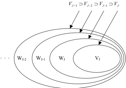
Equation (5) is known as a multi-resolution decomposition of f(t) because the terms of different scales represent the components of the signal at different resolutions. Just as VJ,
WJ, WJ-1, ... , W1 can be seen as a partition of the information set depicted in Figure 1, this information decomposition allows us to reconstruct the signal, f(t), based a subset of relevant information at the jth level of resolution, via the approximation,
) ( ) ( ) ( ) ( 1 t S t D t D t Sj− = J + J +K+ j
These approximations range from the smoothest scale (lowest level of resolution), 2J to finer scales,
2J-1, 2 J-2. ... , 2.
Figure 1 Decomposition of Information starting from Level J
J J J J V V V V −3 ⊃ −2 ⊃ −1 ⊃ WJ-2 WJ-1 WJ VJ . . .
Using the different multi-resolution approximations S1(t), S2(t), ... , SJ(t), we focus on different features of the signal. SJ(t) gives a view of the signal which reflects how the economic fundamentals underpinning the price and demand in our study affect the overall shape. The finer scale approximations reveal more details as a result of incorporating higher frequency observations and shorter time intervals between observations. Electricity price series have large increases and decreases which seem to occur quite randomly, and which exhibit rapid mean reversion. These short-lived, large price changes have the appearance of outlier patches in the data. Electricity price series are
usually collected every half-hour, with information that has a frequency of greater than a half-an-hour regarded as only having noise value in explaining price. To prevent outliers from leaking into the wavelet coefficients at levels of high resolution, we used the robust smoother-cleaner transform developed by Bruce, Donoho, Gao and Martin (1994), a fast wavelet decomposition that is robust to outliers. To implement this wavelet
decomposition we start with a set of smooth wavelet coefficients, say sj. After
calculating a robust set of coefficients, , using running medians of length 5, we derive a robust set of residuals, r
j sˆ j, where ) ˆ ( j j j s s r =δ −
and δ is a shrinkage function which shrinks the coefficients such that
b | x | if b | x | a if a | x | if ) | (| ) ( 0 δ(x) ≥ < < ≤ − − = x a b a x b x sign
We choose the thresholds a and b to ensure that most of the robust residuals are zero. The next level of smooth wavelet coefficients, sj-1, are obtained after applying the usual low-pass wavelet filter to the cleaned smooth coefficients,
uj = sj – rj ,
while we obtain the detail wavelet coefficients, dj-1, by application of the high-pass wavelet filter. This procedure is repeated with the smooth coefficients at the next highest level of resolution. By using the robust smoother-cleaner wavelet transform we remove outlier patches from the decomposition.
A number of key properties of the above procedure make it extremely useful for filtering electricity price series. Firstly, outlier patches of length (2n + 2) are isolated to the wavelet coefficients in frequency levels lower than n. This, in effect, removes the high
and rapidly mean reverting prices from the lower levels. Further, if the distribution of the noise (as distinct from the signal) is the addition of a Gaussian component and some “long-tailed” outlier producing distribution, then Bruce, Donoho, Gao and Martin (1994) show that a further application of the wavelet shrinkage principle8 gives nearly the best possible estimate of f(t), while making a minimum of assumptions about its underlying nature. It is this decomposed series, with outlier patches removed and with wavelet shrinkage applied, that we use as the series to model and base our forecast.
3. ORIGINAL AND RECONSTRUCTED DATA
The data used in this study includes New South Wales electricity spot prices9, as well as the corresponding demand for electricity, all with a sampling frequency of one half-hour. Our sample consisted of observations of system marginal prices and the quantity of electricity demanded, collected between the 17th January, 1998 and 14th August, 1998.10
This period was divided into two; the first 8192 observations forming the basis for our estimation sample, while the remaining 2146 observations comprised the sample held out for forecast evaluation. 11 Figure 2 shows the estimation and holdout samples for the spot prices while Figure 3 displays the corresponding graphs of the demand for electricity series.
Using wavelet analysis as described in the previous section, the price and demand series used for estimation is first decomposed and then reconstructed at different levels of time resolution. To decompose our series we use a biorthogonal wavelet that is robust against leakage of outlier patches in the data into the smooth coefficients.12 The biorthogonal
8 Wavelet shrinkage (see Donoho and Johnstone, 1992) involves first applying a discrete wavelet
transform to the data, then shrinking the wavelet coefficients towards zero before applying the inverse discrete wavelet transform to recover the signal.
9 Electricity spot prices in Australia are known as system marginal prices.
10 The electricity market in NSW is being gradually deregulated. As a result, the structure of the market
exhibits fluidity over time. There is no reason to think that if another estimation and forecast period were to be chosen, the structure would be exactly the same.
11 In this study we made no attempt to bucket the series into either time-of-day or day-of-the-week
categories. This task we left for further research.
12 A biorthogonal wavelet transform utilises both low-pass and high-pass filters. The low-pass filters are
short and avoid outlier leakage to the smooth coefficients. The high-pass filters are long and ensure sufficient smoothness of the underlying basis functions. While biorthogonal wavelets are not orthogonal, for the most part we can use them as we would an orthogonal wavelet.
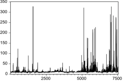
Figure 2 Electricity Spot Price Estimation And Holdout Samples 20 0 40 80 120 160 0 8000 8500 9000 9500 10000 0 50 100 150 200 250 300 350 2500 5000 7500
Spot Electricity Price Estimation Sample Spot Electricity Price Holdout Sample
Figure 3 Electricity Demand Estimation And Holdout Samples
1 4000 5000 6000 7000 8000 9000 10000 11000 12000 2500 5000 7500 5000 6000 7000 8000 9000 10000 1000 8000 8500 9000 9500 10000
wavelet used comes from the "b-spline" family and is coded as bs1.5 in the S+ Wavelets package produced by the StatSci Division of MathSoft and written by Bruce and Gao (1994).13 Both series were decomposed into nine levels of time resolution, cleaned, further waveshrunk, and reconstructed. We employed two types of wavelet shrinkage after first decomposing the estimation series. The first, applies shrinkage to just the highest level of resolution. The effect is not to over-smooth the detail in all but the highest level of resolution. The second applies wavelet shrinkage to all levels of
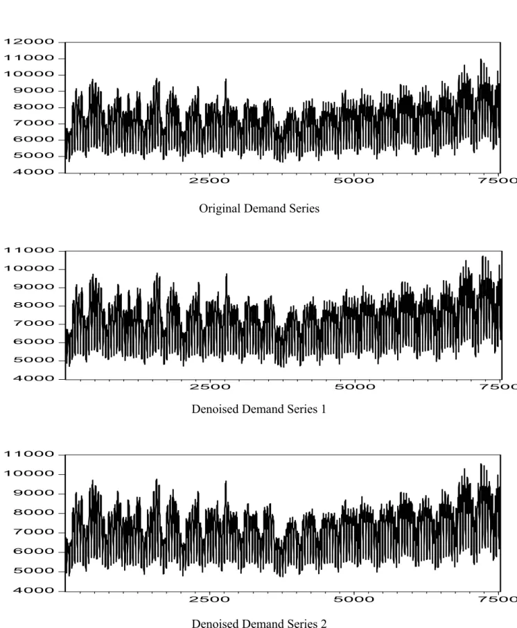
resolution, resulting in a much smoother series. Figure 4 graphically depicts the original estimation price series, the first of the waveshrink filtered series (Denoised Spot Prices 1) and the second filtered series (Denoised Spot Prices 2). The Denoised Spot Prices 2 series in Figure 4 does not appear to be much smoother than Denoised Spot Prices 1. However, when the two series are compared over shorter subsegments of the time horizon, this difference is more obvious. The important message from Figure 4 is the effect that the smoother-cleaner wavelet transform has on reducing the effect of outlier patches in the data by preventing leakage from higher to lower levels of resolution. Figure 5 graphically depicts the corresponding estimation demand series. To control for "edge effects" in the wavelet analysis, the reconstructed data is trimmed to a sample size of 7516 with 338 data points removed from both ends of the series. The estimation sample consists of this reconstructed and trimmed sample. The first 338 points of the forecast series is an ex-post forecast. We know these prices, they were the last 338 prices in the original estimation series that were trimmed after being decomposed and
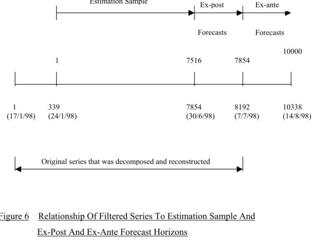
reconstructed. However, forecasts extending from the 7854th time period are truly ex-ante forecasts. The schematic in Figure 6 below outlines on a time line the composition of the estimation sample relative to the sample that was decomposed, along with the ex-post and ex-ante forecast horizons.
Stationarity of all series is assumed in order to estimate the time series models used in this study. The results of Augmented Dickey Fuller (ADF) tests on both the filtered price and demand series confirm the existence of a unit root.14 Accordingly, the first difference of both filtered series is used in our time series modelling to be detailed in the following section.
13 This is the computer package used to decompose and reconstruct the electricity price and demand series. 14 Results of the ADF testing are available from the author on request.
Figure 4 Electricity Spot Price Estimation Series And Denoised Prices 0 50 100 150 200 250 300 350 2500 5000 7500
Original Spot Prices
0 50 100 150 200 250 300 2500 5000 7500
Denoised Spot Prices 1
0 50 100 150 200 250 300 2500 5000 7500
Figure 5 Electricity Demand Estimation Series And Denoised Demand 4000 5000 6000 7000 8000 9000 10000 11000 12000 2500 5000 7500
Original Demand Series
4000 5000 6000 7000 8000 9000 10000 11000 2500 5000 7500
Denoised Demand Series 1
4000 5000 6000 7000 8000 9000 10000 11000 2500 5000 7500
7516 1 7854 10000 Forecasts Forecasts Ex-ante Ex-post Estimation Sample 1 (17/1/98) 339 (24/1/98) 7854 (30/6/98) 8192 (7/7/98) 10338 (14/8/98)
Original series that was decomposed and reconstructed
Figure 6 Relationship Of Filtered Series To Estimation Sample And Ex-Post And Ex-Ante Forecast Horizons
4. TIME SERIES MODELS AND FORECAST EVALUATION
4.1 Time Series Models
There is a substantial body of recent research which suggests asymmetries in the
relationship between individual stock returns and market indices. As reported in Wiggins (1992), stock portfolios when chosen by different criteria exhibit higher systematic risk in up markets than in down markets. The work of Bhardwaj and Brooks (1993) also
documents evidence of changes in systematic risk. Their research suggests the existence of a nonlinear relationship between the stock market and the business cycle. While electricity prices are not determined by trading on the stock market, as previously mentioned in the introduction, variations in demand for electricity are likely to be influenced by underlying activity or business cycle effects. It follows that levels of demand for electricity should reflect levels in the business cycle. Information that determines demand (or change in demand) will also play a role in determining price (or price change). It follows that asymmetries in electricity prices are likely to be present.
The modelling strategy adopted in this study is to fit a linear autoregressive (AR) model to the filtered changes in electricity prices, as well as to fit a model from the threshold autoregressive (TAR) class. The relationship between price changes is first modelled in the context of the conventional AR model. The response to price increases and decreases in an AR model is forced to be symmetrical. As such, it provides a useful benchmark model against which to evaluate forecasts from a model which allows for asymmetric responses.
The model fitted from the TAR class is a threshold autoregressive switching (TARSW) model. This is a piecewise-linear autoregressive model. For our purposes we consider a model with two regimes. What determines whether a contemporaneous price change belongs to one regime or another, is whether the change in demand for electricity is positive or negative. It follows then that the threshold parameter is zero. If a previous change in demand is positive (negative), then the contemporaneous price change will be assigned to the regime where previous price changes were positive (negative).
The switching model has intuitive appeal as a model capable of capturing the high number and different degrees of price increases and decreases. Domain and Louton (1995, 1997) have used models from Tong's (1990) threshold, autoregressive, open loop (TARSO) class to model threshold autoregressive models of stock returns and real economic activity. The switching model used in this study is best described as a variant of the TARSO class. Whether data belongs to one regime or the other depends on whether prices are increasing or decreasing and the trigger for this is the related demand for electricity variable. Economic theory postulates that price is explained by demand. Then, if we are to forecast using a switching model, we need to be able to accurately forecast demand. With the demand time series not as susceptible to as large and
apparently random mean reverting increases and decreases as is price, it should be more straightforward to model and forecast.
Before discussing the models used in this study, it is important to mention an artefact of our estimation sample data that is also likely to be a feature of electricity prices from other markets in the process of deregulation. From Figure 2, there appears to be a systematic shift in the level and volatility of spot prices in the estimation sample. This
change point occurs at approximately observation 4850 (5/5/98). Clearly, this appears to signal a structural change in the market as this pattern following the change- point in the estimation sample is replicated in the following holdout sample. Khmaladze (1998) acknowledges the change-point problem, or the detection of systematic changes, as an issue to be incorporated into the modelling process for electricity prices. While he deals with this problem using a change-point regression approach, in this study we rely on a dummy variable to at least capture changes in the mean level of the series from where we observe the change-point.
The specification of the threshold autoregressive (TAR) forecasting model for spot electricity price changes, utilised in this study, is described below.
If DDi is the ith change in the demand for electricity, and DPi is the ith first-difference of electricity prices, then
> + − + + − − + + − − + + + − + + − + − + + ≤ + − + + − − + + − − + + + − + + − + − + + = 0 if 2 96 2 48 1 2 2 1 1 0 0 i DD if 1 96 2 48 1 2 2 1 1 0 i DP i DD m i DP m s i DP s s i DP s s i DP s i DP i DP D q i DP q p i DP p p i DP p p i DP p i DP i DP D ε β α β β β β π β ε α α α α α α γ α L L L L L L L L ...(6) The data for spot prices and the demand for electricity is high frequency (half-hourly) and characterised by seasonal, time-of-day and diurnal effects. Therefore, in the TARSW model represented by equation (6) above, we would expect that the number of autoregressive lags present in both regimes, p and s, to be large and more than likely multiples of 48. Accordingly, we set p equal to s and estimated models with lag structures for p that varied from 96 to 288 in multiples of 48. Furthermore, in order to capture any daily persistence in price changes we extended the lag structure in bothregimes to include multiples of 48.15 This resulted in a value of 768 for q and m in equation (6) and accounts for a history of slightly more than two weeks of daily price changes. The lag structure for the AR models of both price changes and changes in demand was chosen to be 672 or two weeks of half-hour data. While aware of the advantages of parsimonious models, given the nature of the data, as well as our prime concern of forecasting ability, lag structures of up to two weeks for the best fitting models may not be uncommon for the data sets under consideration.
In the context of this study, what is of interest is not only forecasting the mean but also the variance. If these models and their forecasts are to be useful for understanding the electricity pricing process for pricing derivatives or for risk management, then forecasting the variance is important. Fundamental to this aim is the ability to suitably evaluate a forecast. This is discussed in the next section.
4.2 Forecast Evaluation
Granger and Newbold (1986) point to three problems associated with forecast
comparisons of the forecast and the actual series. First, if ft is the optimal predictor of Xt, based on a certain information set, then
ft = Xt + et ,
where et is the forecast error. Granger and Newbold (1986) show that, unless et takes the value of zero with probability one, the predictor series, ft, will have a smaller variance than the actual series. An estimate of the variance of the change in electricity prices is a focus of this study. This concern suggests that even if we derive an optimal predictor, then it will underestimate the variance of the actual change in prices. This problem is going to be further exacerbated by the fact that the estimated model we use for forecasting is based on the filtered price and demand series. The second problem
concerns the possibility that the levels of the actual series (filtered spot electricity prices) and the predictor series (filtered demand for electricity) may be cointegrated. If they are cointegrated, then their interrelationship should be modelled using an error correction
15 With the frequency of our data being every half-hour, then a multiple of 48 is a multiple of one day’s set
model. This is not an issue in this study. While our unit root testing revealed that both the electricity price and demand series are I(1) processes and should be modelled in first differences, inclusion of an error correction term is not necessary due to the change in demand only entering the TARSW model as a switching variable. The third problem pointed out by Granger and Newbold (1986) concerns the lack of knowledge as to the minimal attainable forecast error associated with a particular series. Some series, like electricity prices or price changes, are inherently difficult to forecast for reasons advanced previously in the introduction. Forecast results for such series, while less impressive than those associated with more stable series (like the change in demand for electricity), may well be quite satisfactory forecasts under the circumstances. We evaluate the forecasts from both our electricity spot price and demand series, while keeping these evaluation problems in mind.
With all our forecasting models, we adopt Theil's inequality coefficient as a statistic for ex-post evaluation purposes. This statistic is related to the root mean square forecast error, scaled such that it will always fall between zero and one. It is given by
∑
∑
∑
= = = + − = n t n t t t n t t t X n f n f X n 1 1 2 2 1 2 1 1 ) ( 1 U ...(7)If U = 0, then a perfect fit results with Xt = ft for all t. On the other hand, if U = 1, then either Xt = 0 when ft is nonzero or vice-versa, and the forecast is as poor as can be. Theil (1966) observed that the average squared forecast error could be decomposed in the following way and, as result, provided insight as to causes of forecast error.
∑ = − = − + − + − = n t Xt ft X f x f r x f n D 1 2(1 ) 2 ) ( 2 ) ( 2 ) ( 2 σ σ σ σ ...(8)
where X, f,σx andσf are the means and standard deviations of the Xt and ft series, and r is the correlation coefficient. From equation (8), we can define the proportions of
inequality as . 2 ) 1 ( 2 , 2 2 ) ( , 2 2 ) ( n D f x r c U n D f n x s n D f X UM σ σ σ σ − = − = − = U
Clearly UM + US + UC = 1. Theil suggests that the values of UM, US and UC (known as the bias, variance and covariance proportions, respectively) have useful interpretations. The bias proportion, UM, indicates systematic error in that it measures how the average values of the forecasts deviate from the actual values. The variance proportion, US,is a measure of how the forecast reflects the variability of the actual series while, UC,
measures unsystematic error which accounts for the remaining error after deviations from the average have been incorporated into UM.
We use this decomposition to evaluate the ability of our forecasts to capture the mean effects and the variability of the holdout sample.16 For both UM and US, a large value
(above 0.1 to 0.2) would be troubling and would indicate the need for a revision of the forecasting model.
Another desirable evaluation criterion is how well a model predicts turning points in the levels of the actual data. We evaluate our forecasts in this context by comparing both the predicted and the holdout series graphically. Our models are modelled in first-differences of the variables. For forecast evaluation we use the forecast of the levels of the price and demand for electricity, both generated from the forecasted first-differences.
16 We are aware of the Granger and Newbold (1986) criticism of the usefulness of this decomposition.
While we don't question the counter example of an AR(1) model that they use to advance their concerns, we feel that the long AR lags used in our models help negate such criticism.
Further, our models are essentially univariate. While this is clearly the case for the AR model, for the TARSW model, the predictor variable only enters to trigger a switch of regimes.
5. ESTIMATION AND FORECAST EVALUATION
Both the change in the electricity price and demand series are modelled using an AR process as well as and the TARSW model discussed in the previous section. The length of each estimation series is 7,516 half-hour observations. The models are estimated using the estimation series comprising 7516 observations, with another 2484 observations being held out for forecast evaluation. First, we estimate the models that are then used to dynamically forecast17 electricity prices for 2484 time periods ahead (approximately a 50 day time horizon). These dynamic forecasts correspond to the observations that comprise the holdout sample.
5.1 Estimation
Table 1 contains summary statistics for the estimated AR and TARSW models of the difference in the original and the two denoised electricity prices. The switching model specified in the previous section, TARSW, requires a switching variable to determine the movement between different regimes. The variable chosen for such a task is the increase or decrease in demand for electricity. If the TARSW model is to be used, then we require a dynamic forecast of the difference in demand for electricity. Table 2 contains summary statistics for the estimated AR models of the difference in demand for electricity for the original and the two denoised series. For each of the series modelled in Tables 1 and 2, attention has been directed to estimating the best-fitting models as defined by the Akaike Information Criterion (AIC), with a residual series purged of autocorrelation. However, we note that the main purpose of our models lies with forecasting and the best-fitting model is not necessarily the best forecasting model. Then, the objective of estimating a parsimonious and best-fitting model that is designed for hypothesis testing with, perhaps,
17 Dynamic forecasts use previous forecasts to generate future forecasts. This occurs when the number of
steps ahead of the forecast and the chosen lag structure are such that the ability to use past prices from the estimation sample as input for lagged values in the forecasting model is exhausted.
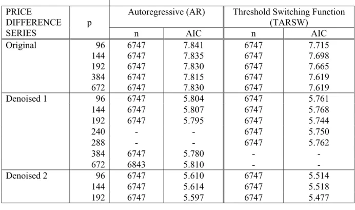
Table 1 Summary Statistics For Estimated AR And TARSW Models Of The Difference In the Original And Denoised Electricity Prices
Autoregressive (AR) Threshold Switching Function (TARSW) PRICE DIFFERENCE SERIES p n AIC n AIC Original 96 6747 7.841 6747 7.715 144 6747 7.835 6747 7.698 192 6747 7.830 6747 7.665 384 6747 7.815 6747 7.619 672 6747 7.830 6747 7.619 96 6747 5.804 6747 5.761 144 6747 5.807 6747 5.768 192 6747 5.795 6747 5.744 240 - - 6747 5.750 288 - - 6747 5.762 384 6747 5.780 - - Denoised 1 672 6843 5.810 - - 96 6747 5.610 6747 5.514 144 6747 5.614 6747 5.518 Denoised 2 192 6747 5.597 6747 5.477
Legend: n = Included observations
AIC = Akaike Information Criterion p = Order of autoregressive terms
a policy making framework in mind, is not of as great a concern in this study as estimating a good forecasting model. As a consequence, we generated forecasts of demand based on AR models of 672 lags using all three series. As previously noted (section 4.1), the lag structure for the AR model was chosen to include a history of two weeks data for the demand for electricity. For part of the forecast horizon, Figure 7 graphically depicts a comparison of the original demand series and the forecast of the Denoised Demand 1 series. The close tracking of the demand series by its forecast is replicated throughout the remainder of the holdout series. A comparison of the original demand series and the forecast of Denoised Demand 2, yields a similar close tracking forecast.
In generating dynamic forecasts of electricity spot prices from TARSW models based on the original prices and the denoised prices 1 and 2, we use the corresponding dynamic forecasts of the original demand and denoised demand 1 and 2 series.
Table 2 Summary Statistics For Estimated AR Models Of The Difference In The Original And Denoised Demand For Electricity
MODEL Autoregressive (AR) DEMAND DIFFERENCE SERIES p n AIC Original 672 6843 10.903 Denoised 1 672 6843 11.179 Denoised 2 672 6843 9.450
Legend: n = Included observations AIC = Akaike Information Criterion p = Order of autoregressive terms
Figure 7 Demand For Electricity And The Dynamic Forecast Of The Denoised Demand 1 Series From Observation 8000 to 8500.
5000 6000 7000 8000 9000 10000 11000 8000 8100 8200 8300 8400 8500
Table 3 Forecast Evaluation Statistics For Forecasts From AR Models Estimated From Original And Denoised Demand For Electricity
MODEL
Autoregressive (AR)
DEMAND
p RMSE MAE MAPE THEIL BIAS VAR COV Original 672 629.0 475.6 0.06 0.04 0.32 0.02 0.66 Denoised 1 672 624.5 472.3 0.06 0.03 0.31 0.01 0.68 Denoised 2 672 607.8 463.4 0.06 0.04 0.31 0.01 0.68
Legend: p = Number of autoregressive parameters RMSE = Root Mean Squared Error
MAE = Mean Absolute Error
MAPE = Mean Absolute Percentage Error THEIL = Theil U Statistic
BIAS = Bias Proportion VAR = Variance Proportion COV = Covariance Proportion
5.2 Forecast Evaluation
Tables 3 and 4 contain forecast evaluation statistics for dynamic forecasts from the demand and price series, respectively.
From Table 3 we observe that the Theil Inequality (U) statistics are low for both the original and the two denoised series. This indicates that the estimated AR models produce fairly accurate forecasts of the demand for electricity.
Accurately forecasting the electricity price is a more difficult task than forecasting change in demand. Recall the Granger and Newbold (1986) warning that some time series are going to be extremely difficult to forecast. The evaluation of forecasts from such series, against those from time series where we can anticipate an accurate forecast, need to be carefully interpreted. The forecasts of the price of electricity, compared to that
Table 4 Forecast Evaluation Statistics For Forecasts From AR And TARSW Models Estimated From Original And Denoised Electricity Prices
MODEL
Autoregressive (AR) Threshold Switching Function (TARSW) PRICES
p RMSE MAE MAPE THEIL BIAS VAR COV RMSE MAE MAPE THEIL BIAS VAR COV Original 96 12.68 9.14 0.35 0.28 0.30 0.18 0.52 130.8 108.89 4.94 0.73 0.67 0.25 0.08 144 16.47 14.18 0.76 0.26 0.52 0.04 0.44 81.61 72.35 3.35 0.62 0.77 0.13 0.10 192 32.83 30.53 1.54 0.40 0.82 0.00 0.18 37.04 32.01 1.52 0.43 0.65 0.10 0.25 384 39.84 31.60 1.49 0.50 0.12 0.42 0.46 45.67 38.90 1.83 0.49 0.60 0.17 0.23 672 90.51 68.98 3.20 0.71 0.09 0.70 0.21 72.42 57.99 2.67 0.61 0.51 0.32 0.17 Denoised 1 96 12.03 8.55 0.32 0.27 0.31 0.42 0.27 47.29 42.82 1.83 0.91 0.81 0.03 0.16 144 16.39 14.03 0.76 0.26 0.56 0.08 0.36 21.21 17.83 0.71 0.53 0.57 0.00 0.43 192 30.76 28.51 1.46 0.38 0.80 0.00 0.20 11.73 7.73 0.37 0.22 0.01 0.04 0.95 240 - - - 12.82 8.95 0.44 0.24 0.01 0.01 0.98 288 - - - 13.60 9.81 0.50 0.24 0.08 0.00 0.91 384 293.3 173.9 7.73 0.91 0.00 0.93 0.07 - - - -672 465.9 258.3 11.45 0.94 0.00 0.95 0.05 - - - -Denoised 2 96 11.27 7.74 0.31 0.24 0.19 0.47 0.34 14.57 11.47 0.55 0.24 0.23 0.00 0.77 144 18.12 16.08 0.85 0.27 0.62 0.05 0.33 13.55 10.32 0.56 0.23 0.31 0.06 0.63 192 30.91 28.61 1.46 0.39 0.79 0.00 0.21 182.6 133.2 5.81 0.94 0.42 0.49 0.09
Legend: p = Number of autoregressive parameters THEIL = Theil U Statistic RMSE = Root Mean Squared Error BIAS = Bias Proportion MAE = Mean Absolute Error VAR = Variance Proportion MAPE = Mean Absolute Percentage Error COV = Covariance Proportion
of the demand for electricity, is one such example where care is required to interpret the evaluation metrics in deciding which series results in the better forecast.
From Table 4, we observe that the dynamic forecast from a TARSW model with an autoregressive lag structure of 192 produces the best set of forecast evaluation statistics. Further, the decomposition of the Theil statistic indicates that this model results in dynamic forecasts that appear to capture the mean and variance components of the price series.
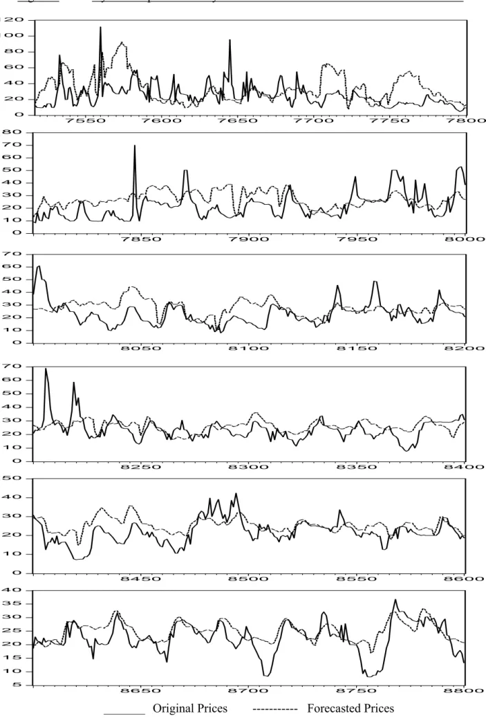
As previously noted, the ability of time series models to forecast turning points is best determined by a graphical representation of the forecasted price against the actual. This representation for dynamic forecasts from the TARSW model is depicted in Figure 8 and Figure 9. The electricity price and demand series were reconstructed using a wavelet shrinkage procedure that shrinks the noise in the highest level of resolution after the application of the robust-smoother discrete wavelet transform. Figures 8 and 9 suggest that after application of this filter, it is possible to generate reasonably accurate forecasts that capture turning points, mean trends and variability.
6. CONCLUSIONS
In this study we have endeavoured to model and forecast the electricity price series for the Australian state of New South Wales from January to August during 1998. To achieve this end, we decomposed our original series using a robust-smoother wavelet transform. Further, we reconstructed the original series using two wavelet shrinkage procedures to obtain two filtered series of electricity prices and demand.
We fitted models from the linear AR and TAR classes to the original and the filtered series. While the model based on the original prices doesn’t adequately forecast the original price, we achieved encouraging results with the forecasts generated from a model estimated from one of the filtered series (Denoised Prices 1). The trade-off is detail for a more fundamental view and forecast of the signal. However, the residual series formed from the difference of
Figure 8 Dynamic Spot Electricity Price Forecasts From Observation 7517 To 8800 0 20 40 60 80 100 120 7550 7600 7650 7700 7750 7800 0 10 20 30 40 50 60 70 80 7850 7900 7950 8000 0 10 20 30 40 50 60 70 8050 8100 8150 8200 0 10 20 30 40 50 60 70 8250 8300 8350 8400 0 10 20 30 40 50 8450 8500 8550 8600 5 10 15 20 25 30 35 40 8650 8700 8750 8800
Figure 9 Dynamic Spot Electricity Price Forecasts From Observation 8801 To 10000 0 20 40 60 80 100 8800 8850 8900 8950 9000 0 10 20 30 40 50 9050 9100 9150 9200 0 40 80 120 160 200 9200 9250 9300 9350 9400 5 10 15 20 25 30 35 9450 9500 9550 9600 0 10 20 30 40 50 9650 9700 9750 9800 0 10 20 30 40 50 60 9850 9900 9950 10000
the original spot electricity prices and their underlying forecasts, offers us an opportunity to model the more intense volatility patches in the data. Recall the last paragraph of Section 2, where we hypothesised that the distribution of these residuals (or “noise”) might be
represented as the addition of a Guassian component and some “long-tailed” outlier
producing distribution. Khmaladze (1998) proposed that the equivalent residual series in his study had a marginal distribution that was best approximated by a mixture of normals. Not only is the modelling of the distribution of this residual series important from the perspective of forecasting price volatility, but it also provides a key to deriving adequate VAR estimates. From this series we can derive an estimate of the potential loss distribution and, as a
consequence, estimates of the expected loss, the unexpected loss and VAR. We leave this extension of our study for future research.
If our interest is in understanding the pricing process of electricity price derivatives through modelling and forecasting price volatility, or developing forecasting models for risk
management of portfolios containing these derivatives then, perhaps, this trade-off between underlying price movements and more detailed forecasts is worthwhile.
REFERENCES:
Bhardwaj, R. and L. Brooks (1993), "Dual Betas From Bull and Bear Markets: Reversal of the Size Effect," Journal of Financial Research, 16: 269-283.
Bruce, A. and H. Gao (1994), S+Wavelets User Manual, StatSci Division, MathSoft Inc., Seattle, Washington, U.S.A.
Bruce, A., Donoho, D., Gao, H. and R. Douglas Martin (1994), "Denoising and robust nonlinear wavelet analysis," SPIE Proceedings, Wavelet Application, 2242, April, Orlando, FL, U.S.A.
Clewlow, L. and C. Strickland (2000), Energy Derivatives: Pricing and Risk Management, Lacima Publications, London, England.
Daubechies, I. (1992), "Ten Lectures On Wavelets," Society for Industrial and Applied Mathematics, Philadelphia, PA, U.S.A.
Domian, D. and D. Louton (1995), "Business Cycle Asymmetry and the Stock Market," The Quarterly Review of Economics and Finance, 35: 451-466.
Domian, D. and D. Louton (1997), "A Threshold Autoregressive Analysis of Stock Returns and Real Economic Activity," International Review of Economics and Finance, 6(2):
Donoho, D. and I. Johnstone (1992), “Minimax estimation via wavelet shrinkage,” Technical Report 402, Stanford University, California, U.S.A.
Granger, C. and P. Newbold (1986), Forecasting Economic Time Series, Academic Press, 2nd Edition.
Khmaladze, E.(1998), “Statistical Analysis of Electricity Prices,” Department of Statistics Report No. S98-11, University Of New South Wales, Sydney, Australia.
Lin, S. and M. Stevenson (2001), "Wavelet Analysis of Index Prices in Futures and Cash Markets: Implication for the Cost-Of-Carry Model," forthcoming in Studies in Nonlinear Dynamics and Econometrics.
Ramsey, J. and C. Lampart (1998), "The Decomposition of Economic Relationships by Time Scale Using Wavelets: Expenditure and Income." Studies in Nonlinear Dynamics and Econometrics 31: 23-42.
Rogers, L. and S. Satchell, (1996) “Does the Behaviour of the Asset Tell Us Anything About the Option Price Formula?” University of Bath, United Kingdom.
Theil, H.(1966), Applied Economic Forecasting, Amsterdam North Holland.
Tong, H.(1990), Non-Linear Time Series: A Dynamical System Approach, Oxford: Oxford University Press.
Wiggins, J.(1992), "Betas in Up and Down Markets," Financial Review, 27: 107-123. Wilkinson, L. and J. Winsen (2000), “Statistical Analysis of N.S.W. Electricity Prices,”
Department of Economics, University of Newcastle, Australia, November.