Energy Slices: Benchmarking with Time Slicing

Scholarship@Western

Electrical and Computer Engineering Publications

Electrical and Computer Engineering Department

2018

Energy Slices: Benchmarking with Time Slicing

Katarina Grolinger

Western University, [email protected]

Hany F. ElYamany

Wilson Higashino

Miriam AM Capretz

Luke Seewald

Follow this and additional works at:

https://ir.lib.uwo.ca/electricalpub

Part of the

Artificial Intelligence and Robotics Commons

,

Computer Engineering Commons

,

Electrical and Computer Engineering Commons

,

Software Engineering Commons

, and the

Sustainability Commons

Citation of this paper:

Grolinger, Katarina; ElYamany, Hany F.; Higashino, Wilson; Capretz, Miriam AM; and Seewald, Luke, "Energy Slices: Benchmarking with Time Slicing" (2018).Electrical and Computer Engineering Publications. 158.

ORIGINAL ARTICLE

Energy slices: benchmarking with time slicing

Katarina Grolinger &Hany F. ElYamany&

Wilson A. Higashino&Miriam A. M. Capretz&

Luke Seewald

Received: 27 March 2017 / Accepted: 25 October 2017 / Published online: 13 December 2017

#The Author(s) 2017. This article is an open access publication

Abstract Benchmarking makes it possible to identify

low-performing buildings, establishes a baseline for measuring performance improvements, enables setting of energy conservation targets, and encourages energy savings by creating a competitive environment. Statisti-cal approaches evaluate building energy efficiency by comparing measured energy consumption to other sim-ilar buildings typically using annual measurements. However, it is important to consider different time pe-riods in benchmarking because of differences in their

consumption patterns. For example, an office can be efficient during the night, but inefficient during operat-ing hours due to occupants’wasteful behavior. More-over, benchmarking studies often use a single regression model for different building categories. Selecting the regression model based on actual data would ensure that the model fits the data well. Consequently, this paper proposes Energy Slices, an energy benchmarking ap-proach with time slicing for existing buildings. Time slicing enables separation of time periods with different consumption patterns. The regression model suited for the specific scenario is selected using cross validation, which ensures that the model performs well on previ-ously unseen data. The evaluation is carried out on a case study involving two sports arenas; event energy efficiency is benchmarked to identify low-performing events. The case study demonstrates the Energy Slice procedure and shows the importance of model selection.

Keywords Energy benchmarking . Energy score .

Energy efficiency . Energy Star . Energy Slices . Energy prediction

Introduction

Buildings account for about 40% of global energy con-sumption and approximately one-third of greenhouse gas emissions (UNEP2011). Moreover, existing build-ings have been recognized as a crucial factor in

K. Grolinger (*)

:

:

:

Department of Electrical and Computer Engineering, Western University, London, ON N6A 5B9, Canada

e-mail: [email protected] H. F. ElYamany e-mail: [email protected] W. A. Higashino e-mail: [email protected] M. A. M. Capretz e-mail: [email protected] H. F. ElYamany

Department of Computer Science, Suez Canal University, Ismailia, Egypt

L. Seewald

London Hydro, London, ON N6A 4H6, Canada e-mail: [email protected]

achieving aggressive targets for reducing greenhouse gas emissions (Europian Union 2012). Consequently, energy efficiency efforts in this domain can have a major impact on relieving growing energy challenges.

The importance of conserving energy in tandem with recent advancements in sensor technology has resulted in wide expansion of smart metering systems. In the electricity domain, smart meters measure electricity con-sumption at intervals of 1 hour or less and communicate that information to a central or cloud system. In addition to enabling analysis of energy consumption patterns, these data create opportunities for new ways of energy performance assessment and benchmarking.

Benchmarking is a way of evaluating a building’s energy performance by comparing its energy consump-tion against its own past performance, against similar buildings, or against a performance indicator (Capozzoli et al.2016). It identifies low-performing buildings for retrofit prioritization, establishes a baseline for measur-ing performance improvements and for evaluatmeasur-ing on-going commissioning, enables setting of targets for en-ergy improvements, and creates a competitive environ-ment to encourage and promote energy savings. Build-ings of the same design may be difficult to compare due to upgrades, differences in occupancy, building use, or climate. By using standardized scores, benchmarking simplifies comparisons among buildings and enables in-sights required to identify energy savings opportunities.

Benchmarking approaches can besimulation model-basedwhen the benchmark is calculated using a model of building energy performance, orstatisticalwhen data for similar buildings are used to generate a benchmark (Gao and Malkawi2014). The advantage of the simula-tion model-based approach is that it can be used before the building is built; however, the disadvantage is that it requires detailed information about the building design and may not accurately reflect actual building use. Sta-tistical approaches require a reasonably sized dataset of similar existing buildings with their historical energy consumption. This approach incorporates occupants’ behavior because it uses actual energy consumption data: more economical behavior results in a better score. Statistical approaches are commonly used for benchmarking existing buildings (Li et al.2014). The Energy Slices approach proposed in this study also belongs to this category.

The actual energy consumption used in benchmarking can be obtained from energy bills or through metering and submetering. Bills and whole-building methods

include the energy consumed by all subsystems, whereas submetering enables analysis according to different end use points (disaggregation may also be used to identify subloads from whole-building metering virtually). Both approaches aggregate consumption for specific time pe-riods: for example, bill-based approaches usually consid-er annual or monthly enconsid-ergy consumption. Nevconsid-ertheless, it is also important to consider the time component in benchmarking methodologies. For instance, a school may be very efficient over the weekend, but inefficient during weekdays due to occupants’wasteful behavior. Similarly, an office building may show different behavior during working and non-working hours. Including the time com-ponent in energy benchmarking can provide a way of determining low-performing time periods and assist in identifying opportunities for improvement.

Based on this observation, this paper proposes Ener-gy Slices, an enerEner-gy benchmarking approach with time slicing for existing buildings. By assigning energy con-sumption data to different time slices, the Energy Slices approach enables independent evaluation of periods with different consumption patterns. In addition, by including a procedure to select the best regression model for a specific scenario and using cross validation, the proposed approach also overcomes two other weak-nesses of existing statistical benchmarking solutions.

The first weakness relates to the fact that most energy benchmarking studies use a single regression algorithm, such as multiple linear regression, support vector regres-sion, or neural networks. In some cases, a different regression model is built for each building category, but each time, the same regression type is used. For example, Energy Star (Hsu2016; Lucid2016) creates a separate regression model for each building type, but they are all based on ordinary weighted least squares. This limitation hinders benchmarking effectiveness be-cause different building types and time slices may be better represented by different models. For instance, linear models (simple, multiple, weighted linear regres-sion, and others) assume a linear correlation between the response variable (energy consumption, energy intensi-ty, or similar) and the independent variables. When this assumption is broken, the model does not represent the data accurately. In contrast, the Energy Slice approach includes a way to choose the regression model that best suits the data being modeled.

The second resolved weakness is that most regres-sion models for benchmarking are built using data from a set of existing buildings (the training set), and then all

buildings are evaluated using this model. This approach, however, may cause overfitting: even though the model represents the training data closely, its performance on unseen data is poor. Hong (2014) highlighted the im-portance of out-of-sample testing in energy forecasting, but this also applies to benchmarking when the model may memorize the training data rather than learning to generalize. To alleviate overfitting and assess how the model will generalize to previously unseen data, this work uses cross validation. Moreover, cross validation provides a way of selecting the regression model as well as its parameters.

The rest of this paper is organized as follows:

BBackground^ introduces linear regression, support vector regression, neural networks, and random forest models, andBRelated work^reviews related work. The proposed Energy Slice benchmarking approach is pre-sented inBEnergy Slices.^An evaluation using a case study involving two sports arenas is presented in

BEvaluation,^andBConclusions^concludes the paper.

are characterized by soft margins; they do not penalize observations within the ɛ deviation from the model prediction (Ben-David and Shalev-Shwartz 2014; Hastie et al.2009).

Given an input spacefðXi;YiÞgii¼¼N1} whereNis the

number of observations, the main goal of SVR is to find a function that deviates at mostɛfrom each observation. The general case of SVR can be described as follows:

Y ¼W⋅Φð Þ þX b; ð2Þ

where Φ(X) is a kernel function that non-linearly maps from the input spaceXto a feature space. Coeffi-cientsWandbare determined as part of the optimization problem that aims to capture observation points within theɛboundary from the predicted value.

Neural networks

Neural networks (NN) (Ben-David and Shalev-Shwartz

2014) are supervised learning models inspired by the human brain. NNs are composed of interconnected neu-rons that can approximate non-linear relationships be-tween input and output variables. Like an SVM, an NN can be used for regression and classification. A common way of representing NNs is with graphs whose nodes are the neurons and whose edges correspond to interactions between them, with arrows pointing in the direction of data transfer among neurons (Hastie et al.2009).

One of the most common NNs, the feedforward neural network (FFNN), is composed of a flexible num-ber of layers: an input layer, one or more hidden layers, and an output layer. Information moves from the input layer through the hidden layer(s) to the output layer. Each neuron in the input layer represents a feature in the input data space, and the number of neurons in the output layer is equal to the number of output variables. The output of each neuron in a hidden or output layer is determined as follows:

yj¼φ ∑Ni¼1wijxiþwio

; ð3Þ

where thexiare the neuron inputs, thewijare synaptic

weights connecting the i-th neuron in the input (or hidden) layer to the j-th neuron in the next hidden (or output) layer, and wiois a bias that shifts the decision

boundary, but does not depend on any input. φis an activation function that is usually modelled as a step or as a sigmoid function. During the training phase, weights are adjusted (learned) using backpropagation Background

This section introduces the four machine learning ap-proaches used in this work: linear regression (LR), support vector regression (SVR), neural networks (NN), and random forest (RF).

Linear regression

Linear regression (LR) (Hastie et al.2009) models the relationship between independent and dependent or pre-dictor variables using a linear function. Withn indepen-dent variables, the model takes the following form (Ben-David and Shalev-Shwartz2014):

y_i¼a0þa1xi1þa2xi2…þanxin; ð1Þ

where yi is the i-th dependent variable, {xi1,xi2,…

xin}are the independent variables, and (a0,a1,a2,…an) are vectors of regression coefficients of sizen+ 1 esti-mated from data.

Support vector regression

Support vector regression (SVR) (Basak et al.2007) is a subcategory of support vector machine (SVM) learning models that is used for regression. Both SVM and SVR

together with an optimization method such as gradient descent.

Random forests

Random forests (RF) (Breiman 2001) are a type of ensemble learning model composed of individual deci-sion trees that are used for both classification and re-gression. In an RF, each individual tree is trained by an algorithmAon different, but possibly overlapping, parts of the same training data setS.For example, an RF can be an ensemble of B trees {T1(X),…,TB(X)}, where

X= {x1,…,xn} is ann-dimensional feature vector. Each

tree may be using a different algorithm and a different part of the data set.

The final prediction is obtained by combining the prediction outcomes from all individual trees (Ben-Da-vid and Shalev-Shwartz 2014). In the example of B

trees, the ensemble produces B outputs

^

Y1¼T1ð ÞX ;…;Y^B ¼TBð ÞX ;

, where Y^a, a= 1, …,B, is the value predicted by thea-th tree. The final predictionY^ is made by averaging the predicted values of each tree.

Related work

Several survey papers have discussed the problem of benchmarking building energy consumption (Chung

2011; Li et al.2014; Pérez-Lombard et al.2009) and reviewed various concepts involved in assessing build-ing energy efficiency, includbuild-ing benchmarkbuild-ing, energy rating, and energy labeling. They also discussed the development of an energy certification scheme and highlighted main considerations such as what and how it should be calculated.

Chung (2011) discussed mathematical methods used in developing benchmarking systems; examples of the models considered include regression models, stochas-tic frontier analysis, and data envelope analysis. Each method was analyzed to identify its strengths and weak-nesses. The author also presented a literature review of how these methods and their variants have been used for building energy benchmarking.

Li et al. (2014) reviewed methods for benchmarking building energy consumption against its past or intended performance. They classified the methods presented into three categories: white, gray, and black box methods. Black box methods use data fitting approaches (e.g.,

linear regression and neural networks) and therefore require large quantities of data for training; statistical approaches belong to this category. White box ap-proaches are based on physical properties of building components and require extensive design documenta-tion; simulation is an example from this category. Gray box methods fall between white and black boxes; they use data fitting together with knowledge of the physical building.

The surveys mentioned (Chung2011; Li et al.2014; Pérez-Lombard et al.2009) included discussion of var-ious statistical approaches and the use of measured energy consumption for benchmarking. However, these approaches do not include a way to select the regression model that is best suited for a specific benchmarking scenario. Moreover, the Energy Slice benchmarking approach presented in our work includes time slicing, which enables separate assessment of periods with dif-ferent consumption characteristics.

Palmer and Walls (2017) assessed the role of benchmarking and disclosure policies adopted in 15 US cities in decreasing energy use and CO2emissions.

They observed that disclosing other energy information in addition to the Energy Star score is needed. Palmer and Walls also noted that the Energy Star Portfolio Manager has been criticized for using overly small and non-current data set to build the model and not capturing building heterogeneity. Their work highlights (Palmer and Walls2017) the need for improved benchmarking.

Gao and Malkawi (2014) proposed a benchmarking solution based on intelligent clustering. The proposed benchmarking process starts by using ak-means algo-rithm to classify buildings based on selected features such as area and operating schedule. The resulting clusters contain buildings with similar characteristics. A building’s efficiency is indicated by how far it is from the centroid of the cluster to which it belongs. However, like the reviewed surveys (Chung2011; Li et al. 2014; Pérez-Lombard et al. 2009), Gao and Malkawi (2014) did not consider how to select the b e s t s u i t e d r e g r e s s i o n m o d e l f o r s p e c i f i c benchmarking scenarios or to benchmark over time slices.

Capozzoli et al. (2016) presented a methodology for benchmarking annual energy consumption of health-care centers. The methodology presented consists of two main phases: the first phase segments the heteroge-neous health-care centers into homogeheteroge-neous classes using a classification and regression tree (CART). Next,

a linear mixed-effect model is constructed to combine the effects of the input variables. The second phase involves using Monte Carlo simulation to determine the benchmarking value by evaluating the frequency distribution for each class individually. A drawback of this methodology is that it is based on a linear model, which may not reflect reality. In addition, unlike our approach, Capozzoli et al. (2016) did not address sepa-rate benchmarking for different time periods.

Khayatian et al. (2016) evaluated annual energy per-formance of residential buildings based on neural net-works. They focused on determining the optimal subset of input features, the number of NN layers, and the number of neurons. These features were extracted from previously defined energy certificates issued by a municipality in Italy. Although most benchmarking methods are concerned with overall building energy consumption, Khayatian et al. (2016) focused specifi-cally on heating energy consumption. Again, time slices and algorithm selection were not considered.

Wang (2015) proposed a building energy efficiency benchmarking approach based on Technique for Or-der Preference by Similarity to Ideal Solution (TOPSIS). Instead of depending on only one criterion, Wang took a multi-criteria approach and included several measurements in the benchmarking process, such as energy intensity per unit of space and energy use per individual occupant. Weights were assigned to energy performance indicators using a combination of principal component analysis (PCA) and multiple lin-ear regression (MLR). Each building was compared to the most and the least energy efficient buildings in terms of multiple indicators in an attempt to achieve a more comprehensive evaluation. Whereas Wang (2015) considered space size and number of occupants through multiple performance indicators, our ap-proach incorporates these dimensions as input vari-ables of the statistical model.

In addition, numerous implementations of building energy benchmarking systems have been developed, such as the Energy Star system proposed in the USA and Canada (ENERGY STAR2016; Natural Resources Canada2011), Cal-Arch in the USA (U.S. Department of Energy 2015a), and Energy Smart Office Label in Singapore (Lee and Priyadarsini2008). Moreover, re-cent case studies have discussed establishing energy benchmarking baselines for buildings in specific regions worldwide. For example, Yang and Zhang (2016) used a statistical approach to determine the benchmarking

baseline for existing residential buildings in China. Juaidi et al. (2016) also used a statistical approach to perform energy benchmarking analysis, but for shop-ping centers in the Gulf Coast region. Morris et al. (2016) applied multiple linear regression models to benchmark electricity and gas consumption for households across England. Finally, Shabunko et al. (2016) carried out a benchmarking energy analysis for residential buildings in Brunei Darussalam using the EnergyPlus simulation tool (U.S. Department of Energy2015b). Furthermore, a number of building en-vironmental assessment schemes have been developed, including the Leadership in Energy and Environmental Design (LEED) (USGBC2014) in the USA and Cana-da, the Eco-Management and Audit Scheme (EMAS) (European-Commission2017) in the European Union, the Building Owners and Managers Association Build-ing Environmental Standards (BOMA BEST) (BuildBuild-ing Owners and Managers Association of Canada2013) in Canada, and the Building Research Establishment En-vironmental Assessment Methodology (BREEAM) (BREEAM 2017) in the UK. Lee and Priyadarsini (2008) reviewed assessment schemes and showed that assessments typically account for performance-based criteria (such as annual energy use and greenhouse gas emissions) and feature-based criteria (such as types of walls and roofs).

All the reviewed studies contribute to the building benchmarking domain in diverse ways, but unlike our work, they do not consider how to select the statistical model that is best suited for the benchmarking scenario. Moreover, our work uses time slicing to evaluate time periods with different energy use characteristics separately.

Energy Slices

The main objective of this work is to design a generic benchmarking approach that can be used to evaluate the energy efficiency of different buildings as well as to assess the efficiency of distinct time slices. Like Energy Star (Lucid2016), the Energy Slice approach proposed here includes building a regression model, calculating an energy efficiency ratio, and fitting a probability dis-tribution. However, where Energy Star uses ordinary least squares regression, the Energy Slice approach in-cludes a procedure for selecting the regression model and ensuring that the model will be generalized to

unseen data. Moreover, time slicing enables consider-ation of diverse time periods.

The proposed Energy Slice approach is illustrated in Fig.1. It consists of two flows: the first one,building benchmarking system, is responsible for creating a sta-tistical model to evaluate energy efficiency relative to a peer group. Its outputs are a regression model and a

cumulative probability distribution. The second flow,

energy efficiency scoring, is responsible for calculating an energy efficiency score using the regression model and probability distribution provided by the first flow. Details of the proposed flows are provided in the fol-lowing subsections.

Building benchmarking system

Building the benchmarking system involves taking a data set consisting of energy consumption measure-ments together with contextual information to create artifacts needed for the energy efficiency scoring.

Inputs

Energy consumptiondata in the Energy Slice approach are obtained from smart meters. This is a crucial require-ment because it enables time slicing and therefore sep-aration of time periods with different occupants’ behav-iors. For instance, in the case of office buildings, hourly (or finer granularity) consumption data make it possible to associate consumption with operating hours.

Like other energy benchmarking solutions, this work also uses weather conditions and building

attributes as input. Building energy benchmarking typically considers weather through heating and cooling degree days (Li et al.2014). In contrast, time slicing requires finer-grained weather data corre-sponding to observed time segments. For example, energy consumption to maintain a comfortable office may be very different if the outside temperature is− 10 °C or + 25 °C. Consequently, the granularity of the weather data is determined by the size of the time slices and energy reading intervals: there should be at least one weather reading for each time slice con-sidered, but there is no need for more frequent tem-perature readings than energy readings. Local hourly weather data are available from a variety of service providers through APIs such as those from Weather Underground (2017).Building attributesare similar to those in a typical whole building benchmarking sys-tem (Lucid 2016); depending on the benchmarking objective, they may include building size, number of occupants, number of floors, number of rooms, and other factors.

Finally,time slice attributesconstitute the impor-tant differentiating factor from other building benchmarking approaches: they describe the context of a specific time slice or period. For example, if benchmarking working and non-working hours for an office building, time slice attributes describe these periods and include attributes such as duration, num-ber of people in the building, operating equipment, and time of day. These are closely related to the ob-jectives of benchmarking and time slicing because they describe the context of specific time periods.

Data preparation

The data preparation step consists of time slicing and attribute selection. Time slicing determines the seg-ments of time that should be considered separately in the benchmarking process. In the case of office build-ings, working and non-working hours could be con-sidered separately. If the objective is to benchmark the energy efficiency of events in conference venues, each event should be considered as a separate time slice. Time slices do not necessarily need to be of the same duration, but if they are not, this needs to be accounted for in the regression model by including attributes that describe slice duration. Moreover, time slices do not have to be continuous: for example, anBoffice hours^ slice may contain all periods corresponding to work-ing hours.

Each time slice represents a single data point for the regression model, therefore other attributes (features) need to describe the time period captured by the slice. The four categories of input attributes are processed differently. Energy consumption data from smart meters or other sensors are summarized to represent total consumption in the period indicated by the slice.Weather conditionmust be processed to arrive at a single value for each time slice. In the case where time slice duration is in the range of hours, weather attributes may include average temperature, humidity, and wind speed. When a time slice spans several seasons, as in the case of benchmarking an-nual consumption for working and non-working hours, other measures such as degree days can be used.Building attributesare not dynamic and there-fore are used Bas is.^ Time slice attributes describe the context of the time slice and, like weather condi-tions and energy consumption, have a single value for a time slice. Duration must be included whenever time slices are of different lengths.

Attribute selectionaims to select the relevant attri-butes for benchmarking. It can be carried out using filter methods based on measures such as mutual information or using wrapper methods that rely on predictive models to score feature subsets. Although principal component analysis (PCA) is not strictly an attribute selection meth-od, but an attribute reduction technique, it can also be used. PCA takes possibly correlated variables and ap-plies an orthogonal transformation to create a set of linearly uncorrelated variables referred to asprincipal components (Hastie et al. 2009). Dimensionality is

reduced by using only the firstnprincipal components. When the number of attributes is small, attribute selec-tion may not be necessary, and all available attributes can be used for benchmarking.

Regression algorithm construction

This step consists of two parts: regression algorithm selection and building the regression model. In regres-sion algorithm selection, the regression algorithm that provides the best representation of the available data is selected. Note that building regression models on the complete data set and choosing the one with the lowest error rate on the training set may lead to overfitting. To avoid overfitting and biased estimation, the out-of-sample evaluation must be performed; the regression model must be evaluated on data that were not used to build the model. Specifically, the proposed Energy Slice approach uses k-fold cross validation to evaluate the regression models and select the best one, as illustrated

in Fig.2.k-fold cross validation was chosen over the holdout method (simply splitting data into training and validation subsets) because it remedies training-testing split bias and takes advantage of all available data.

For each algorithm from a set of candidate algorithms (steps 1 and 2), k-fold cross validation executes the following steps: the data set is split into ksubsets of equal size (step 3). The number of folds equals the number of subsetsk. One subsetkis reserved for vali-dation, the model is trained on the remaining subsets (step 4), and error is calculated on the validation subsetk

(step 5). The process is repeatedktimes, each time using a different validation set (steps 6, 4, and 5). The algo-rithm performance for previously unseen data is esti-mated as the average error over all folds (step 7).

Mean absolute percentage error (MAPE) and the coefficient of variance (CV) are used as error measures. MAPE was chosen because it is a relatively easily understandable measure. It expresses accuracy as a per-centage and is calculated as follows:

εa¼MAPE¼ 1 N ∑ N i¼1 yi−^yi y_i ; ð4Þ

whereyiis the actual consumption,^yi is the predicted

consumption, andNis the number of observations. The coefficient of variance (CV) is used as the sec-ond measure. The CV measure has often been used in energy prediction studies (Grolinger et al. 2016); it expresses error variation with respect to the mean and is calculated as follows: CV ¼ ffiffiffiffiffiffiffiffiffiffiffiffiffiffiffiffiffiffiffiffiffiffiffiffiffiffiffiffiffiffiffiffiffiffi 1 N−1 ∑ N i¼1 yi−^yi 2 s y 100; ð5Þ

whereyi,^yi, andN represent the same elements as in

MAPE andyis the average actual consumption. MAPE and CV errors are estimated for all candidate algorithms, and the algorithm with the lowest error is selected for benchmarking.

Algorithms such as SVR have several parameters that must be selected for optimal model performance. In the Energy Slice approach, parameter selection is performed using grid search as part of the training performed in step 4, as shown in Fig.2. Combinations of possible parameter values form a grid, and k-fold cross validation is performed for each grid element.

The combination with minimum error is selected as the optimal one. Grolinger et al. (2016) have used this method to select parameters for energy consumption and demand prediction.

Therefore, there are two nestedk-fold cross valida-tions in the regression algorithm selection procedure: an outer one evaluates the accuracy of each candidate algorithm as illustrated in Fig.2, and an inner one selects the appropriate model parameters, which is performed as part of step 4.

After the regression algorithm has been selected, the process continues by building the regression model. During the algorithm selection stage, training was al-ways performed only on a part of the data set because one subset was reserved for evaluation. Now, the regres-sion model is built with the algorithm and parameters selected in the regression algorithm selection step, but with the complete data set. By using the complete set, the model benefits from all available data.

As illustrated in Fig.1, the output of this step is the regression model that will be used for energy efficiency scoring. The same model is used to score the entities that were used to build it and for new data.

Calculating energy efficiency ratio

The regression model enables calculation of expected/ predicted energy consumption and consequently of the

energy efficiency ratio(EER). EER is the ratio between actual and expected energy consumption and is calcu-lated as follows:

EER¼y

^

y

^; ð6Þ

where y and ^y are the actual and expected (or predicted/ regression) energy consumptions for a time slice. The predicted energy consumption^yis obtained from the regression model. EER values greater than one indicate performance below the expectation, and values less than one denote performance above the expectation for specified conditions.

Note that an EER score is calculated for each time slice for each building considered. For instance, when time slices are working and non-working days, each building will have two EERs, one for working and one for non-working days. When benchmarking events from a conference venue, each event will have its own EER value.

Energy Star also calculates the energy efficiency ratio by dividing actual by predicted energy (Environmental Protection Agency2014). However, in Energy Star,yand

^

yare the actual and predictedannual source energy use intensities.Source energyis the amount of raw fuel that is required to operate the building (Environmental Protection Agency2014). In the Energy Slice approach,

yand^yare not annual measures, but actual and predicted consumptions for a specific time slice. Moreover, Energy Star converts site energy into source energy to account for the use of different types of energy. The Energy Slice approach is flexible because it can be used for different energy types as long as similar things are compared. For example, the electrical efficiency of working and non-working hours for different office buildings can be com-pared if they use the same sources of energy. To compare overall energy efficiency among buildings with different sources of energy, the source energy should be used.

Fitting cumulative probability distribution

The energy efficiency ratio provides an indication of efficiency, but does not denote efficiency relative to a group of peers. To establish a score from 1 to 100 indicating the standing of a sample relative to its group, a cumulative distribution function must be fitted to the data. On this scale, higher numbers indicate better ener-gy efficiency.

This step is similar to Energy Star distribution fitting. Energy efficiency ratios are sorted from smallest to largest, and the cumulative percentage of the population in each ratio is calculated. A cumulative probability distribution(CPD) is then fitted to the data. The CPD is the artifact that will be used for energy efficiency scoring.

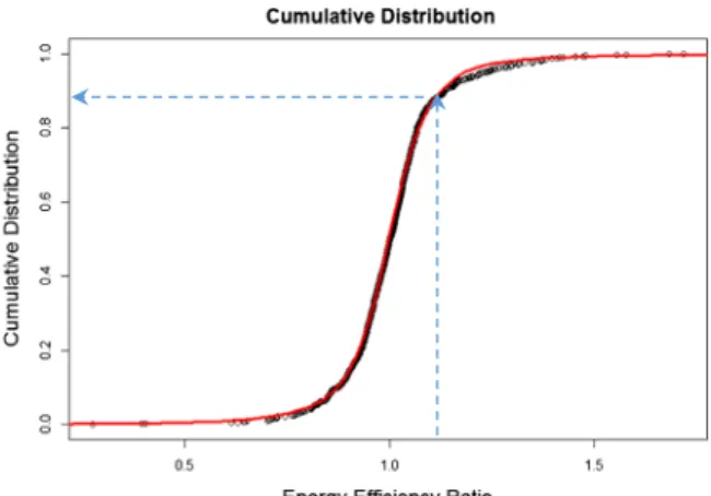
Figure3shows an example of distribution fitting for SVR: the dots represent the calculated cumulative dis-tribution values. Values towards the left part of the graph represent higher efficiency. The solid red line is the fitted CPD.

To select the CPD function from a set of candidates, the Akaike information criterion (AIC) is used (Akaike

2011). This criterion was chosen over others such as the Kolmogorov-Smirnov test and the Anderson-Darling test, because it discourages overfitting by penalizing models with large numbers of parameters. Therefore, it provides a trade-off between model goodness of fit and its complexity. AIC evaluates the relative quality of statistical models: it estimates model quality in

comparison to other models, but it does not assess absolute quality. If all candidate models are inaccurate, AIC will still choose the best one. Therefore, quantile-quantile (Q-Q) plots can also be used to assess the distributions with top AIC values.

Energy efficiency scoring

After the regression model has been created and the cumulative probability distribution has been fitted to the data, the model is ready to score energy efficiency. Scoring can be carried out on the same data that were used for building the benchmarking system as well as on new data. When the model is used for the same data, the preparation step has already been completed, as illus-trated in Fig. 1, and the data are ready for energy efficiency calculation.

New data, or data that were not used to build the system, must have the same attributes as the data used to build the model. Inputs should include energy consump-tion, weather conditions, building attributes, and time slice attributes.

To match the structure of the data used to build the benchmarking system, new data must undergo data preparation. This involves only time slicing; attribute selection process, which was part of data preparation during system construction, is not performed here be-cause the attributes have already been selected. The time slicing step performed during energy efficiency scoring is the same as the one in building the benchmarking system (BData preparation^).

Next, the expected (predicted) energy^yis calculated for new and/or old data using the regression model. The

exact calculation depends on the regression model and the selected regression algorithm. Subsequently, the en-ergy efficiency ratio is obtained according to Eq. (6).

Next, for each entity with its corresponding energy efficiency ratio, the cumulative distribution value (CDV) is calculated based on the fitted distribution function. This step is illustrated in Fig.3 with dashed lines. The obtained cumulative distribution values are on a scale from 0 to 1.

Finally, the Energy Efficiency Scores (EES) are cal-culated as follows:

Evaluation

This section presents an evaluation of the Energy Slice approach described in this paper by using it to assess the energy consumption efficiency of events that were held in two entertainment arenas in Canada. Identify-ing low-performIdentify-ing events assists in findIdentify-ing opportu-nities for energy improvement and promotes energy efficiency.

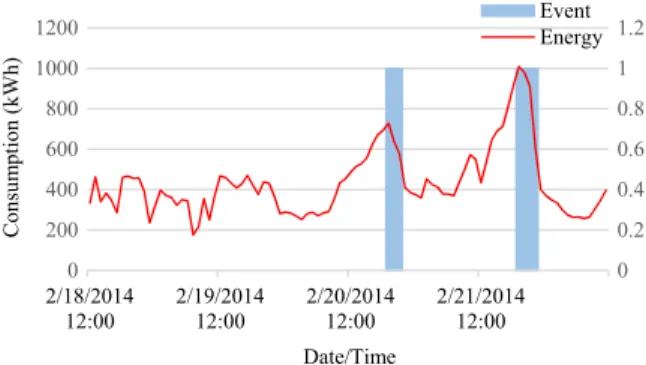
Figure 4 illustrates electricity consumption over a few days in one of these arenas, with vertical bars representing event duration. It can be observed that the patterns are very different for event and non-event days. During event days, an increase in energy consumption

starts in the morning, and its peak can reach several times that of a non-event day. Therefore, it is important to consider the efficiency of individual events.

The data set used in the experiments consisted of 795 events that were held between January 1, 2012 and April 20, 2016 in two Canadian entertainment arenas: Budweiser Gardens, located in London, ON, and GM Centre, located in Oshawa, ON. The data set contained a variety of events, such as hockey and basketball games, concerts, and musical performances.

All experiments were implemented in the R language (R Cor e Te am 2014). The Bstats,^ Be1 071 ,^

Brandomforest,^ and Bneuralnet^ packages were used to implement LR, SVR, RF, and NN, respectively.

BInputs and data preparation^ discusses the data set used and the data preparation. BRegression algorithm construction^ discusses regression algorithm construc-tion, and BCalculating energy efficiency ratios and fitting the cumulative probability distribution^presents the results of the distribution fitting experiments. Final-ly,BBenchmarking results^presents the benchmarking results, andBDiscussion^compares them with an alter-native formulation in which event setup (preparation) was also considered.

Inputs and data preparation

Input data were prepared for benchmarking by using the time slicing procedure. Table1presents an over-view of the prepared attributes for each event. Because the number of available attributes was relatively small,attribute selectionwas not carried out, and all attributes were used for benchmarking.

The attributes were classified asenergy consumption,

weather conditions,building attributes, and time slice attributes as defined in BBuilding benchmarking system.^ Note that each event represents only a time slice of the total arena energy consumption. Other benchmarking solutions consider aggregate annual or monthly data only, which hinders their ability to evalu-ate specific time periods.

Energy consumptiondata were obtained through the Green Button standard interface (North American Energy Standards Board 2016). London Hydro, the local electrical utility involved with this project, has developed the first cloud-based Green Button Connect My Data test environment to enable data access to academic partners with the customer’s consent. Data were originally recorded at 15-min intervals for both

0 0.2 0.4 0.6 0.8 1 1.2 0 200 400 600 800 1000 1200 2/18/2014 12:00 2/19/2014 12:00 2/20/2014 12:00 2/21/2014 12:00 Consum ption (kW h) Date/Time Event Energy

Fig. 4 Energy consumption and events

EES¼ð1−CDVÞ*100; ð7Þ where CDV is the cumulative distribution value. The resulting efficiency scores range from 0 for the worst performers to 100 for the best performers. For example, a score of 70 corresponds to the 0.3 point in the cumu-lative distribution and indicates that only 30% of the population performed better than the sample being evaluated.

arenas. The energy consumption of an event was calcu-lated as the aggregate consumption for the event duration.

Weather condition data were obtained from the Weather Underground (2017) and represent the average temperature and humidity during each event.

Thebuilding attributesgroup in this case study only included building size as square footage. It is possible to include other attributes that possibly impact energy con-sumption, such as a number of offices or the size of open spaces.

Time slice attributesdescribe the context of a specific time slice. Because in this case study time slices repre-sent individual events, time slice attributes are used to describe events. For instance, the event schedule is captured by attributes including day of year, hour of day, and day of week. The arena seating configuration, which indicates the maximum seating capacity for a specific setup, was used as an approximation of event attendance because attendance was not available. Regression algorithm construction

After the data were prepared, building the benchmarking system continued by selecting the regression model that best described the available data.

To demonstrate the importance of the algorithm se-lection step, the experiments in this section considered four regression methods: LR, SVR, NN, and RF. To show that it is not sufficient to evaluate models on the complete data set and to provide evidence that

out-of-sample evaluation is necessary, each algorithm was assessed in two ways:

& Without k-fold: training was carried out on the com-plete data set, and the error rate was evaluated on the same set. Similar procedures are typically used by existing benchmarking solutions (Environmental Protection Agency 2014; Hong2014). However, calculating the error on the same data set that was used for training is not considered proper statistical evaluation (Hastie et al.2009).

& With k-fold: training and evaluation were carried out according to k-fold (k= 5) cross validation and therefore followed proper statistical procedures by considering an out-of-sample evaluation. The re-ported values are the average of allk-fold trainings a s d e s c r i b e d i n BR e g r e s s i o n a l g o r i t h m construction.^

Table2shows the MAPE and CV error metrics for all four methods, with and withoutk-fold evaluation. Note that for both cases and for each training round, grid search with k-fold evaluation was also used to select the best parameters for each algorithm.

Table 2 shows that withoutk-fold cross validation, the RF method was the one with the lowest error ac-cording to both MAPE and CV measures. However, when k-fold cross validation was included, SVR was the method with the best performance. These results show the importance of performing a thorough analysis of regression models. RF would have been chosen if the

Table 1 Event attributes

Group Name Data type Description

Energy consumption consumption double Total energy consumption

Weather conditions temperature int Average temperature during the event humidity int Average humidity during the event Building attributes sqft int Building square footage

Time slice attributes dayOfYear int Event day of the year dayOfWeek int Event day of the week hourOfDay int Event start hour duration int Event duration in minutes hockey boolean Indicates if event is a hockey game basketball boolean Indicates if event is a basketball game

other boolean Indicates if event is neither a hockey nor a basketball game

training had been performed over the entire data set and evaluated on the same set, but thek-fold cross validation showed that SVR had better generalization capacity. Without thek-fold cross validation, the selected model would have fit the training data very well, but it would have performed poorly on previously unseen data. This demonstrates the need for out-of-sample evaluation, specifically cross validation, when selecting a regression model.

Based on the results shown in Table 2, SVR was selected as the regression method for event benchmarking. Next, the regression model was built with the selected algorithm and with the complete data set. Rebuilding the selected model in this way makes use of all available data.

Calculating energy efficiency ratios and fitting the cumulative probability distribution

The regression model, in this case study, the one built using SVR, enables calculation of the expected/ predicted energy consumption for each event. Based on these predictions, the energy efficiency ratios (EERs) can also be obtained, as described by Eq. (6). Finally, fitting a cumulative probability distribution to the calculated EERs transforms the EERs into energy efficiency scores.

To select a cumulative distribution, the AIC values for candidate distributions were calculated using theBpropagate^ package in R. Table3 shows the top five distributions and their corresponding AIC values. It can be observed that the AIC values for the top two distributions, scaled/shifted t and Johnson SU, are quite close. Therefore, their fit to the observed data was analyzed using quantile-quantile (Q-Q) plots. Figure 5 shows Q-Q plots for the Johnson SU and shifted/scaled t distributions.

For the middle range of energy efficiency ratios, both Johnson SU andtdistributions fit the data very well. For low and high ranges of EER, there is a divergence from the optimum line for both Johnson SU and shifted/scaled t distributions. Nevertheless, for high EER values, the shifted/scaledtdistribution fit the data better than the Johnson SU distribution, which corroborates the AIC values obtained. Benchmarking results

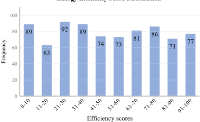
Based on the selected regression model (SVR) and fitted cumulative distribution (shifted/scaled t distribution), the energy efficiency scores for all events were calcu-lated as described inBEnergy efficiency scoring.^ Fig-ure6shows the resulting score distribution, which has an almost uniform shape. The average score was 49.58, and the standard deviation was 28.87.

The scores were further analyzed to validate the results. Figure7shows the events’energy consump-tion versus their energy efficiency scores. Data points of different color and shape are used to dif-ferentiate among hockey, basketball, and other types of events. The graph shows that hockey games tended to consume more energy than other events. This was expected because maintaining ice requires relatively large electricity consumption. In particu-lar, most hockey games consumed much more elec-tricity than basketball games. Nevertheless, this did not result in hockey games having lower scores than basketball games. As illustrated in Fig.7, efficiency scores for both hockey and basketball games varied from very low to very high. Some hockey games achieved similar energy efficiency scores to basket-ball games while consuming much more energy (the hockey curve is to the right from the basketball one). This is a desirable behavior because the nature of hockey events drives higher energy consumption, and they should not be directly compared with

bas-Table 2 MAPE and CV errors for the four algorithms with and withoutk-fold cross validation

MAPE CV

Withoutk-fold Withk-fold Withoutk-fold Withk-fold

LR 14.28 14.50 21.22 21.63

SVR 9.18 11.65 15.93 20.39

NN 12.18 12.98 18.04 20.78

RF 6.80 12.51 10.94 21.22

Table 3 Top five distributions according to AIC

Distribution AIC Scaled/shiftedt −128.2381240 Johnson SU −126.0873096 Logistic −84.5754229 3P Weibull −42.9829251 Skewed-normal −37.1996307

ketball events.

Example 1 in Table4shows two events A and B, respectively: a hockey and a basketball game. Al-though the hockey event energy consumption is much higher than the basketball event consumption, both received the same score. This is because hockey events are expected to consume more electricity due to their nature. This example together with Fig. 7

demonstrates that the proposed benchmarking ap-proach can differentiate among various types of events and benchmark them appropriately.

The Energy Slice approach also showed good ca-pability to differentiate between efficient and ineffi-cient events within a single category. For instance, hockey games consumed on average 15.3 kWh per minute of an event. The top 10 scored hockey games consumed only 12.45 kWh, whereas the bottom 10 consumed 24.22 kWh. A similar observation applies

to basketball games. The average energy consumption for a basketball game was 10.17 kWh per minute. The top 10 energy consuming games used on average 8.98 kWh per minute, whereas the bottom 10 con-sumed on average 12.19 kWh per minute.

Example 2 in Table4compares two hockey events. Although their energy consumptions are quite similar, the events received very different scores, 81 and 9. However, the event attributes indicate that the average temperature during event C was 25 °C, whereas dur-ing event D was 14 °C. Because hockey events require much more electricity for cooling the ice when the outside temperature is high, it can be expected that consumption would be significantly greater for higher temperatures. Therefore, although event C had similar consumption to event D, it received a much higher score (81) because it achieved this consumption dur-ing a higher temperature period. This demonstrates

Fig. 5 Q-Q plots for Johnson SU and shifted/scaledtdistribution

that the Energy Slice approach can also account for event context, specifically outdoor temperature. Discussion

The experiments described in the previous subsections showed that the Energy Slice approach developed in this research can be effectively used to score the energy efficiency of time slices of entertainment arenas (events).

Obviously, the greatest difficulty in developing a benchmarking approach is to assess its quality. To the best of the authors’knowledge, there is no other ap-proach that could be used in the same context and therefore compared with this research.

Nonetheless, BRegression algorithm construction^

demonstrated the need for the algorithm selection step described in Fig.2, andBBenchmarking results^ dem-onstrated that the resulting scores conform to intuition. Moreover, scores were independently assessed by spe-cialists from the local electricity distribution company

and the facility operators. These specialists believed the scores produced were coherent and could be successful-ly related to differences in comparable event operations. However, to evaluate the Energy Slice approach in more depth, two additional experiments were conduct-ed. The first one compared scores when different regres-sion algorithms were used. In the second experiment, the benchmarking behavior for a different time slicing approach was analyzed.

Experiment 1

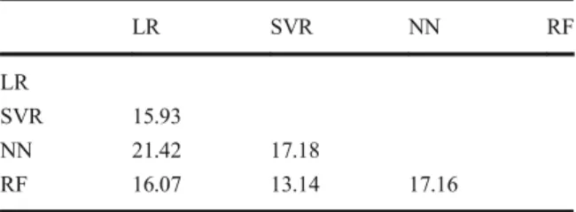
Table 5 compares efficiency scores obtained with dif-ferent algorithms. Each cell contains the average abso-lute difference between the scores produced by the algorithms in the corresponding row and column. For instance, the average absolute difference between LR and SVR scores is 15.93. Note that the absolute differ-ence is used because otherwise the average could be-come approximately zero by summing negative and positive differences.

The smallest difference was 13.14 between SVR and RF. This indicates that if RF algorithm was selected instead of SVR, the difference in final scores would be on average 13.14. Similarly, if LR was used instead of SVR, the difference in final scores would be on average 15.93. These experiments demonstrated the importance of using out-of-sample evaluation for algorithm selec-tion described in Fig. 2 and the impact of algorithm selection on the final score.

Experiment 2

In this experiment, the scores were recalculated consid-ering the time slice of an event from the start of its setup (preparation) to its end time. The reasoning behind this experiment is that the increase in energy consumption due to event setup should be included in the efficiency evaluation. This contrasts with the previous experi-ments, which considered only the event duration (event start to event end) as the time slice. To enable this analysis, the following attributes were also added:

& Setup duration, containing the duration of event setup in minutes

& Setup temperature, containing the average tempera-ture during event setup

& Setup humidity, containing the average humidity during event setup

89 63 92 ₈₉ 74 73 81 86 71 77 0 20 40 60 80 100 Frequency Efficiency scores

Energy Efficiency Score Distribution

Fig. 6 Energy efficiency score distribution

0 20 40 60 80 100 0 2000 4000 6000 8000

Energy Efficiency Score

Energy Consumption (kWh)

Energy Consumption vs Score

Hockey Basketball Others

In addition, the total event energy consumption was also updated to include consumption during event setup. Figure8shows how the original and updated scores compare with each other. The average absolute score difference was 16.83, and the standard deviation was 15.38. There were 53 events whose scores were un-changed. Several events experienced a large change: score decrease indicates inefficiencies in setup whereas increase denotes energy efficient setup.

Figure 9 shows a histogram of the (non-absolute) score differences. Most events lie in the range [− 20,20], which demonstrates that the Energy Slice ap-proach is stable with regard to changes in the time slicing. Nevertheless, the histogram also shows that approximately one-third of the events had larger chang-es in their scorchang-es.

Figure10helps to understand these larger changes better. In this graph, the x-axis represents the setup duration relative to the event duration, whereas they -axis represents the setup energy consumption relative to the event consumption. The dashed black line rep-resents the data points in which the relationship be-tween these variables is one. On this line, one unit of increase in duration represents a proportional increase in energy consumption. Therefore, the data points below the dashed line represent events that are spend-ing less energy on setup than expected. Conversely,

the data points above the line represent events with less efficient setup.

The graph shows that, once again, the benchmarking results comply with intuition. Blue circle data points represent the 30 events that had the largest increase in score by considering event setup in the time slice. Note that most of these data points are below the black line (they had efficient setups). On the other hand, points marked by red diamonds represent the 30 events with the largest decrease in score. In this case, they are mostly above the line. For the sake of comparison, all events with no change in the score are also plotted.

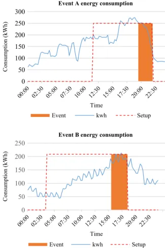
To explore changes in efficiency scores in more depth, two events, event A from the bottom 30 and event B from the top 30, were analyzed. Figure 11

shows their energy consumption together with event and setup duration. Event A exhibited very high energy consumption during setup, even exceeding the con-sumption during the event. On the other side, event B was much more efficient during the preparation stage, as indicated by lower energy consumption. Consequently, event A’s score decreased, whereas event B’s score increased when setup was included in the observations.

Conclusions

This paper has presented Energy Slices, a novel statistics-based benchmarking approach that con-siders time slices of building energy consumption. By doing so, this approach can analyze different time periods of a building’s operation and find new opportunities for improvement and cost reduction. For instance, an office building may have different levels of efficiency during working and non-working periods due to the wasteful behavior of its occupants. Benchmarking solutions that analyze monthly or yearly data may not detect this

Table 4 Event efficiency score

examples Date and time Event type Temp. (°C) Consumption (kWh) Score

Example 1 Event A 2013-10-11 19:30 Hockey 14 2436.53 55 Event B 2013-11-09 19:00 Basketball 10 1414.35 55 Example 2 Event C 2012-08-31 19:30 Hockey 25 2974.50 81 Event D 2014-10-15 19:00 Hockey 14 2997.43 9

Table 5 Differences among energy efficiency scores with differ-ent algorithms LR SVR NN RF LR SVR 15.93 NN 21.42 17.18 RF 16.07 13.14 17.16

inefficiency because they consider only aggregated information.

In addition to time-slicing capabilities, the Energy Slice approach also includes a procedure to select the regression model that best describes the analyzed data. This procedure aims to guarantee that the baseline used in the energy efficiency ratio calculation accurately rep-resents the group of buildings under consideration. This approach contrasts with existing benchmarking process-es that use a single model type for every building type and scenario.

Finally, the Energy Slice approach was evaluated through a case study in which events occurring in Ca-nadian entertainment arenas were benchmarked. The results show that the Energy Slice approach is robust and produces scores for events that are consistent with their energy consumption efficiency.

Traditionally, benchmarking assesses the building energy performance by assigning a score that can be used for retrofit prioritization, goal setting, and improve-ments evaluation. Time slice approach goes beyond traditional benchmarking by providing the ability to

0 20 40 60 80 100 0 20 40 60 80 100 Score (w/ setup) Original Score

Original Score vs Score (w/ setup)

Fig. 8 Original scores versus scores considering event setup

0 6 29 114 265 ₂₅₉ 82 32 8 0 0 50 100 150 200 250 300 Fr eq u en cy Score difference Score Difference

Fig. 9 Histogram of differences between original scores and scores considering event setup

0 1 2 3 4 5 6 0 1 2 3 4 5 6 S etup co nsum pti o n (r el ativ e to e v en t co nsumptio n )

Setup duration (relative to event duration)

Setup duration vs Setup Consumption

No Change Bottom 30 Top 30

Fig. 10 Relative setup duration versus relative increase in energy consumption 0 50 100 150 200 250 300 Time

Event A energy consumption

Event kwh Setup 0 50 100 150 200 250 Consumption (kWh) Consumption (kWh) Time

Event B energy consumption

Event kwh Setup

identify low-performing time periods, and therefore, it assists in identifying improvement opportunities.

Future work will explore the application of the pro-posed approach to different scenarios such as separate evaluation of office working and non-working hours or assessment of energy performance in different seasons.

References

Akaike, H. (2011). Akaike’s information criterion. In M. Lovric (Ed),International Encyclopedia of Statistical Science. Berlin, Heidelberg: Springer Berlin Heidelberg.https://doi. org/10.1007/978-3-642-04898-2_110.

Basak, D., Pal, S., & Patranabis, D. C. (2007). Support vector regression.Neural Information Processing - Letters and Reviews, 11(10), 203–224. https://doi.org/10.4258 /hir.2010.16.4.224.

Ben-David, S., & Shalev-Shwartz, S. (2014).Understanding ma-chine learning: from theory to algorithms. New York: Cambridge University Press. https://doi.org/10.1017 /CBO978110729801.

BREEAM. (2017). Building research establishment environmen-tal assessment method.http://www.breeam.com/. Accessed 18 Mar 2017.

Breiman, L. (2001). Random forest.Machine Learning, 45(1), 1– 33.https://doi.org/10.1017/CBO9781107415324.004. Building Owners and Managers Association of Canada. (2013).

Building environmental standards.http://bomacanada. ca/bomabest/. Accessed 18 Mar 2017.

Capozzoli, A., Piscitelli, M. S., Neri, F., Grassi, D., & Serale, G. (2016). A novel methodology for energy performance benchmarking of buildings by means of linear mixed effect model: the case of space and DHW heating of out-patient healthcare centres. Applied Energy, 171, 592–607. https://doi.org/10.1016/j.apenergy.2016.03.083.

Chung, W. (2011). Review of building energy-use performance benchmarking methodologies.Applied Energy, 88(5), 1470– 1479.https://doi.org/10.1016/j.apenergy.2010.11.022. ENERGY STAR (2016). The Simple Choice for Energy

Efficiency.https://www.energystar.gov/. Accessed 18 Mar 2017.

Environmental Protection Agency (2014). ENERGY STAR score: technical reference.https://portfoliomanager.energystar. gov/pdf/reference/ENERGYSTAR Score.pdf. Accessed 18 Mar 2017.

European-Commission (2017). Eco-management and audit s c h e m e ( E M A S ) . h t t p : / / e c . e u r o p a . eu/environment/emas/index_en.htm. Accessed 18 Mar 2017. Europian Union. (2012). Directive 2012/27/EU of the European Parliament and of the Council of 25 October 2012 on energy efficiency. Official Journal of the European Union, 55(L315), 1–56http://data.europa.eu/eli/dir/2012/27/oj. Gao, X., & Malkawi, A. (2014). A new methodology for building

energy performance benchmarking: an approach based on intelligent clustering algorithm.Energy and Buildings, 84, 607–616.https://doi.org/10.1016/j.enbuild.2014.08.030. Grolinger, K., L’Heureux, A., Capretz, M. A. M., & Seewald, L.

(2016). Energy forecasting for event venues: big data and prediction accuracy.Energy and Buildings, 112, 222–233. Hastie, T., Tibshirani, R., & Friedman, J. (2009).The elements of

statistical learning data mining, inference, and prediction, 2nd Edition. New York: Springer-Verlag New York. https://doi.org/10.1007/b94608.

Hong, T. (2014). Energy forecasting: past, present, and future. Foresight: The International Journal of Applied Forecasting, 32, 43–48.

Hsu, D. (2016). Improving energy benchmarking with self- re-ported data.Building Research & Information, 42(5), 641– 656.https://doi.org/10.1080/09613218.2014.887612. Juaidi, A., AlFaris, F., Montoya, F. G., & Manzano-Agugliaro, F.

(2016). Energy benchmarking for shopping centers in Gulf Coast region. Energy Policy, 91, 247–255. https://doi. org/10.1016/j.enpol.2016.01.012.

Khayatian, F., Sarto, L., & Dall’O’, G. (2016). Application of neural networks for evaluating energy performance certifi-cates of residential buildings.Energy and Buildings, 125, 45– 54.

Lee, S. E., & Priyadarsini, R. (2008). Building energy efficiency labelling programme in Singapore.Energy Policy, 36(10), 3982–3992.

Li, Z., Han, Y., & Xu, P. (2014). Methods for benchmarking building energy consumption against its past or intended performance: an overview.Applied Energy, 124, 325–334. https://doi.org/10.1016/j.apenergy.2014.03.020.

Lucid (2016). Energy Star Portfolio Manager. https://www. e n e r g y s t a r. g o v / b u i l d i n g s / f a c i l i t y o w n e r s a n d -managers/existing-buildings/use-portfolio-manager. Accessed 18 Mar 2017.

Morris, J., Allinson, D., Harrison, J., & Lomas, K. J. (2016). Benchmarking and tracking domestic gas and electricity Acknowledgments The authors would like to thank London

Hydro for supplying industry knowledge, the Green Button plat-form, and the data used in this study. They also would like to thank Budweiser Gardens and GM Centre for providing valuable data for this project.

FundingThis research has been partially supported by an NSERC (Natural Sciences and Engineering Research Council of Canada) CRD at Western University (CRD 477530-14).

Compliance with ethical standards

Conflict of interest Author Miriam A.M. Capretz has received a research grant from NSERC. There are no other conflicts of interest.

Open AccessThis article is distributed under the terms of the Creative Commons Attribution 4.0 International License (http:// creativecommons.org/licenses/by/4.0/), which permits unrestrict-ed use, distribution, and reproduction in any munrestrict-edium, providunrestrict-ed you give appropriate credit to the original author(s) and the source, provide a link to the Creative Commons license, and indicate if changes were made.

consumption at the local authority level.Energy Efficiency, 9(3), 723–743.https://doi.org/10.1007/s12053-015-9393-8. Natural Resources Canada (2011). About ENERGY STAR.http://

www.nrcan.gc.ca/energy/products/energystar/about/12529. Accessed 18 Mar 2017.

North American Energy Standards Board (2016). Green Button. http://energy.gov/data/green-button. Accessed 18 Mar 2017. Palmer, K., & Walls, M. (2017). Using information to close the energy efficiency gap: a review of benchmarking and disclo-sure ordinances. Energy Efficiency, 10(3), 673–691. https://doi.org/10.1007/s12053-016-9480-5.

Pérez-Lombard, L., Ortiz, J., González, R., & Maestre, I. R. (2009). A review of benchmarking, rating and labelling con-cepts within the framework of building energy certification schemes.Energy and Buildings, 41(3), 272–278.https://doi. org/10.1016/j.enbuild.2008.10.004.

R Core Team. (2014). In http://www.r-project.org/ (Ed.),R: a language and environment for statistical computing. Vienna: R Foundation for Statistical Computing.

Shabunko, V., Lim, C. M., & Mathew, S. (2016). EnergyPlus models for the benchmarking of residential buildings in Brunei Darussalam. Energy and Buildings.https://doi. org/10.1016/j.enbuild.2016.03.039.

U.S. Department of Energy. (2015a). High-performance buildings f o r h i g h - t e c h i n d u s t r i e s . h t t p s : / / h i g h t e c h . l b l .

gov/resources/calarch-california-building-energy. Accessed 18 Mar 2017.

U.S. Department of Energy (2015b). Building technologies office: EnergyPlus Energy Simulation Software. Energy Efficiency and Renewable Energy. http://apps1.eere.energy. gov/buildings/energyplus/?utm_source=EnergyPlus&utm_ medium=redirect&utm_ca mpaign=EnergyPlus%2 Bredirect%2B1. Accessed 18 Mar 2017.

UNEP (2011). Sustainable buildings and climate initiative: pro-moting policies and practices for the built environment. http://staging.unep.org/SBCI/pdfs/SBCI_2pager_280112_ english_web.pdf. Accessed 18 Mar 2017.

USGBC (2014). Leadership in energy and environmental design. http://www.usgbc.org/leed. Accessed 18 Mar 2017. Wang, E. (2015). Benchmarking whole-building energy

perfor-mance with multi-criteria technique for order preference by similarity to ideal solution using a selective objective-weighting approach. Applied Energy, 146, 92–103. https://doi.org/10.1016/j.apenergy.2015.02.048.

Weather Underground (2017). Weather forecast reports. https://www.wunderground.com/. Accessed 18 Mar 2017. Yang, T., & Zhang, X. (2016). Benchmarking the building energy

consumption and solar energy trade-offs of residential neigh-borhoods on Chongming Eco-Island, China.Applied Energy, 1 8 0, 7 9 2–7 9 9 . h t t p s : / / d o i . o r g / 1 0 . 1 0 1 6 / j . apenergy.2016.08.039.