2012
Mining maximal cliques from large graphs using
MapReduce
Michael Steven Svendsen
Iowa State UniversityFollow this and additional works at:
https://lib.dr.iastate.edu/etd
Part of the
Computer Engineering Commons, and the
Computer Sciences Commons
This Thesis is brought to you for free and open access by the Iowa State University Capstones, Theses and Dissertations at Iowa State University Digital Repository. It has been accepted for inclusion in Graduate Theses and Dissertations by an authorized administrator of Iowa State University Digital Repository. For more information, please [email protected].
Recommended Citation
Svendsen, Michael Steven, "Mining maximal cliques from large graphs using MapReduce" (2012).Graduate Theses and Dissertations. 12624.
by
Michael Steven Svendsen
A thesis submitted to the graduate faculty
in partial fulfillment of the requirements for the degree of MASTER OF SCIENCE
Major: Computer Engineering
Program of Study Committee: Srikanta Tirthapura, Major Professor
David Fernandez-Baca Daji Qiao
Iowa State University Ames, Iowa
2012
DEDICATION
I would like to dedicate this thesis to my parents. Whose love, support, and kind financial assistance has carried me through the years. I would also like to dedicate this work to my wife Jennifer, who would just smile and listen as I babbled on about cliques and MapReduce.
TABLE OF CONTENTS LIST OF TABLES . . . v LIST OF FIGURES . . . vi ACKNOWLEDGEMENTS . . . vii ABSTRACT . . . viii CHAPTER 1. INTRODUCTION . . . 1 CHAPTER 2. PRELIMINARIES . . . 3 2.1 Notation . . . 3 2.2 MapReduce . . . 3
2.3 Tomita et al. Sequential MCE Algorithm . . . 5
CHAPTER 3. REVIEW OF LITERATURE . . . 7
3.1 Review of Sequential Algorithms for MCE . . . 7
3.2 Review of Parallel Algorithms for MCE . . . 10
3.3 Parallel Frameworks . . . 11
3.3.1 Pregel . . . 11
3.3.2 Dryad . . . 11
3.3.3 MPI . . . 12
CHAPTER 4. TECHNICAL APPROACH . . . 13
4.1 Na¨ıve Parallel Algorithm . . . 13
4.2 Na¨ıve Algorithm Deficiency . . . 13
4.3 Algorithm Enhancement . . . 15
4.5 Correctness of PECO . . . 19
4.6 PECO and Other Parallel Frameworks . . . 20
4.6.1 Pregel . . . 21
4.6.2 Dryad . . . 21
4.6.3 MPI . . . 21
CHAPTER 5. RESULTS . . . 22
5.1 Ordering Strategy Evaluation . . . 23
5.1.1 Strategy comparison . . . 23
5.1.2 Load balancing versus enumeration time reduction . . . 24
5.2 PECO Scalability . . . 28
5.3 Summary and Comparison to Other Algorithms . . . 30
CHAPTER 6. CONCLUSION . . . 32
LIST OF TABLES
Table 5.1 Test graph statistics . . . 23
Table 5.2 Longest reduce task completion times . . . 24
Table 5.3 Total running time comparison . . . 24
Table 5.4 Hypothesis tests . . . 28
LIST OF FIGURES
Figure 2.1 MapReduce data flow . . . 4
Figure 4.1 Na¨ıve algorithm load balancing issues . . . 14
Figure 4.2 Ordering reduce task comparison . . . 16
Figure 5.1 Load balance or reduced enumeration time . . . 25
Figure 5.2 Equal load balance vs. equal enumeration time . . . 26
Figure 5.3 Load balance vs. enumeration reduction . . . 27
Figure 5.4 PECO scalability . . . 29
ACKNOWLEDGEMENTS
I would like to take the opportunity to express my gratitude toward several individuals who have helped me during my graduate education at Iowa State University. I am most appreciative of Dr. Srikanta Tirthapura’s guidance and help with my work on this thesis. I could not have asked for a better research mentor. I would also like to thank the other committee members. I thank Dr. David Fernandez-Baca for participating in several early discussions on this work and whose algorithms class I thoroughly enjoyed taking. I would also like to thank Dr. Daji Qiao, who has helped me throughout my years at Iowa State University, both in the classes he taught and in helping me gain valuable research positions.
ABSTRACT
Maximal clique enumeration (MCE), a fundamental task in graph analysis, can help identify dense substructures within a graph, and has found applications in graphs arising in biological and chemical networks, and more. While MCE is well studied in the sequential case, a single machine can no longer process large graphs arising in todays applications, and effective ways are needed for processing these in parallel.
This work introduces PECO (Parallel Enumeration of Cliques using Ordering); a novel parallel MCE algorithm. Unlike previous works, which require a post-processing step to remove duplicate and non-maximal cliques, PECO enumerates maximal cliques with no duplicates while minimizing work redundancy and eliminating the need for an additional post-processing step. This is achieved by dividing the input graph into smaller overlapping subgraphs, and by inducing a total ordering among the vertices. Then, as a subgraph is processed, the ordering is used in tandem with a sequential MCE algorithm to reduce redundant work while only enumerating a clique if it satisfies a certain condition with respect to the ordering, ensuring that each maximal clique is output exactly once. It is well recognized that in enumerating maximal cliques, the sizes of different subproblems can be non-uniform, and load balancing among the subproblems is a significant issue. Our algorithm uses the above vertex ordering to greatly improve load balancing when compared with straightforward approaches to parallelization.
PECO has been designed and implemented for the MapReduce framework, but this technique is applicable to other parallel frameworks as well.
Our experiments on a variety of large real world graphs, using several ordering strategies, show thatPECO can enumerate cliques in large graphs of well over a million vertices and tens of millions of edges, and that it scales well to at least 64 processors. A comparison of ordering strategies shows that an ordering based on vertex degree performs the best, improving load balance and reducing total work when compared to the other strategies.
CHAPTER 1. INTRODUCTION
Enumerating all maximal cliques in a graph is known as the maximal clique enumeration (MCE) problem. MCE is a fundamental problem in graph theory with many useful applications. It is used for clustering and community detection in social and biological networks [34], the study of the co-expression of genes under stress [36], and used to integrate different types of genome mapping data [16]. Several works use maximal cliques in the study of proteins, examining protein interactions, secondary structure, and sequence clustering [4, 13, 21, 32, 43]. In [17] they are used in comparing the chemical structures of two compounds, and in [28] they are used for mining association rules.
Unfortunately, the number of maximal cliques in a graph can be exponential in the number of vertices [33] and MCE has been proven to be NP-hard [10]. Although this is true in the worst case, not all graphs exhibit this behavior and polynomial time sequential algorithms [2, 3, 6, 10, 11, 12, 18, 20, 29, 39, 40] can be achieved if the number of maximal cliques in the output is polynomial in the input size.
Large graphs are becoming more common, such as web [26] and social network [24] graphs. These graphs often contain millions of vertices and edges, and it is important to process them in parallel to achieve a reasonable turnaround time. In addition, these graphs may not even fit in the memory of a single machine. This motivates the search for parallel and distributed enumeration algorithms.
MapReduce [8] is a parallel framework that has recently gained popularity due to its low cost to setup and maintain, the simple interface provided to the programmer, its built-in fault tolerance, and the availability of open source implementations such as Hadoop [1]. For these reasons, we focus on algorithms that fit the MapReduce model of computation.
of Cliques usingOrdering). To enumerate maximal cliques, PECO (1) divides the graph into overlapping subgraphs, ensuring each maximal clique is contained in at least one of these, and (2) uses a sequential MCE algorithm to process these subgraphs independently and in parallel. To reduce redundant work in computing cliques and ensure each maximal clique is enumerated only once, PECO induces a strict ordering over the vertices of the graph. Work redundancy is then reduced by using this ordering in conjunction with the sequential algorithm, while duplicate enumeration is eliminated by only enumerating a clique if it meets a certain condition of the subgraph and ordering; this ensures the clique is output only once, and the sequential algorithm ensures the clique is maximal.
This work improves on prior work in the area in two ways. First, it outputs only maximal cliques without duplicates while also reducing redundant work in computing cliques, and second, it addresses the issue of load balancing in the distributed environment. Previous works in the area [27, 42] follow the strategy of enumerating maximal, non-maximal, and duplicate cliques with a post-processing step needed to remove the non-maximal and duplicate cliques from the output. This can be a time consuming step, as the final output can be very large, and the presence of duplicates can make the intermediate output even larger. Parallel MCE also faces the problem of non-uniform subproblem size, and it is recognized as a difficult problem to predict the size of these subproblems prior to enumeration [37]. The previous works do not address this load balancing issue. PECO’s vertex ordering strategy, on the other hand, contributes to a balanced load by distributing work relatively evenly across subgraphs. Furthermore, a carefully chosen vertx ordering can reduce the total work performed by the algorithm when compared to na¨ıve ordering schemes by reducing the subproblem sizes.
To demonstrate these improvements, PECO is run on a variety of large real world graphs using several ordering strategies. The results of these experiments show that PECO can enu-merate maximal cliques in large graphs of millions of vertices, and that it scales well to at least 64 processors. A comparison of ordering strategies show that an ordering based on vertex degree performs the best, improving load balance and reducing total work when compared to the other strategies.
CHAPTER 2. PRELIMINARIES
2.1 Notation
Let G = (V, E) be an undirected graph with n = |V| and m = |E|. For v ∈ V, let Γ(v) denote the set{u∈V : (u, v)∈E}, this is also known as the neighborhood ofv. Furthermore, letGv denote the subgraph ofGinduced byv∪Γ(v). Letrankdefine a function whose domain
is V and which assigns an element from a totally ordered universe to each vertex in V. For u, v ∈ V and u 6= v, either rank(u) > rank(v) or rank(v) > rank(u). A subset C ⊆ V is a
clique inG if for every pair of vertices u, w ∈C the edge (u, w) ∈E. A clique C is maximal
in G if no vertex u ∈ V −C can be added to C to form a larger clique. Let µ represent the total number of maximal cliques inG. In the remainder of this work, any reference to a clique refers to a maximal clique, unless otherwise specified. The MCE problem is as follows. Given an undirected graphG, enumerate all maximal cliques inG.
2.2 MapReduce
MapReduce [8] is a framework designed for processing big data sets on clusters consisting of commodity hardware. It has gained wide popularity in industry due to its overall low cost to setup and maintain, the simple interface it provides to the programmer, the system’s built in fault tolerance, and the availability of open source implementations such as Hadoop [1]. For these reasons we selected MapReduce to provide a parallel solution to the MCE problem.
At the core of MapReduce are the map and reduce functions, described by Equations 2.1
and2.2. Themapfunction takes as input a key-value pair (k, v) and emits none, one, or possibly many new key-value pairs (k0, v0). The keys and key-value pairs do not need to be unique. The reduce function processes a particular key k and all values that are associated with k. It
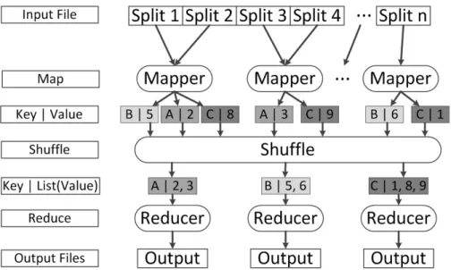
Figure 2.1: Overview of the MapReduce data flow.
outputs a final list of key-value pairs.
map(k, v)→ {(k1, v1),(k2, v2), . . . ,(km, vm)}, m≥0 (2.1)
reduce(k, list(v))→ {(k01, v10), . . . ,(k0m, v0m)}, m≥0 (2.2) The execution of every MapReduce job consists of a map phase, a shuffle phase, and a reduce phase. An overview of the data flow is depicted in Figure2.1. When a job is launched, the input is partitioned intosplits by the framework. These splits are then distributed to map tasks, also known as mappers. A map task is a node in the cluster which executes the map function on each key-value pair in the assigned input split, storing the intermediate results locally. Upon completion, each map task sends all values associated with a particular keykto areduce task assigned to process that key. The process of moving the key-value pairs from the map tasks to the assigned reduce tasks is the shuffle phase. At the completion of the shuffle, all values associated with a key k are located at a single reduce task. This reduce task then runs the reduce function for k. Any key-value pairs emitted by the reduce tasks are written back to the file system as the final output of the job.
The total number of map tasks and reduce tasks is limited by the size of the cluster being used. However, in general the set of keys will be much larger than the number of map tasks
(reduce tasks). Therefore, each task will process a set of keys, running the map (reduce) function once for each key. Even though a task may be responsible for a set of keys, the keys are still processed independently of each other with no state retained from one key to another. A significant feature of MapReduce is its built in fault tolerance. A failure at a particular map or reduce task only impacts the keys at that task, since the keys are not dependent on one another. When the failure is detected, the keys assigned to that task can be easily reassigned to an available node in the cluster. This fault tolerance is built on the notion of independent tasks. As a result, the framework restricts communication between map tasks, as well as communication between reduce tasks. Therefore, the map function must be able to process keys-value pairs independently of any other key-value pairs, likewise thereducefunction must be able to process keys independently of any other keys.
2.3 Tomita et al. Sequential MCE Algorithm
PECO uses the Tomita et al. sequential maximal clique enumeration algorithm (TTT) [39]. The algorithm has a running time of O(3n3), which is worst case optimal. Although only guaranteed to be optimal in the worst case, in practice, it is found to be one of the fastest on typical inputs. A brief overview is given here.
TTT is based on the Bron-Kerbosch depth first search algorithm [2]. Algorithm 1 shows the Tomita recursive function. The function takes as parameters a graph G and the sets K, Cand, and Fini. K is a clique (not necessarily maximal), which the function will extend to a larger clique if possible. Cand is the set{u∈V :u∈Γ(v),∀v∈K}, or simply u∈Cand must be a neighbor of every v ∈K. Therefore, any vertex in Cand could be added toK to make a larger clique. Fini contains all the vertices which were previously in Cand and have already been used to extend the cliqueK.
The base case for the recursion occurs whenCandis empty. IfFiniis also empty, thenK is a maximal clique. If not, then a vertex fromFinicould be added toK to form a larger clique. However, each vertex inFinihas already been explored, adding it would re-explore a previously searched path. Therefore, if Fini is non-empty, the function returns without reporting K as maximal.
Algorithm 1:Tomita(G, K,Cand,Fini)
Input: G- a graph
K - a non-maximal clique to extend
Cand - the set of vertices that could be used to extend K Fini - the set of vertices previously used to extend K 1 if (Cand=∅) & (Fini=∅) then
2 reportK as maximal
3 return
4 end
5 pivot←u∈Cand∪Fini that maximizes the intersectionCand∩Γ(u) 6 Ext←Cand−Γ(pivot)
7 for q∈Extdo
8 Kq ←K∪ {q}
9 Candq←Cand∩Γ(q)
10 Finiq←Fini∩Γ(q)
11 Tomita(G,Kq,Candq,Finiq)
12 Cand←Cand− {q}
13 Fini←Fini∪ {q}
14 K←K− {q} 15 end
Otherwise, at each level of the recursion, a u ∈ Cand ∪Fini with the property that it maximizes the size of Γ(u)∩Cand is selected to be thepivotvertex. The set Extis formed by removing Γ(pivot) fromCand. Each q∈Extis used to extend the current cliqueK by adding q toK and updating theCand and Fini sets. These updated sets are then used to recusively call the function. Upon returning, q is removed from Cand and K, and it is added to Fini. This is repeated for each q∈Ext.
Using the vertices from Ext instead of Cand to extend the clique prunes paths from the search tree that will not lead to new maximal cliques. The vertices in Γ(pivot) can be ignored at this level of recursion as they will be considered for extension when processing the recursive call forK∪ {pivot}. For a formal proof see [39].
One of the key ideas to note here is that no cliques which contain a vertex in Fini will be enumerated by the function. PECOuses this to avoid duplicate enumeration of cliques across reduce tasks. This will be discussed in greater detail in future sections.
CHAPTER 3. REVIEW OF LITERATURE
The sequential MCE problem has been extensively studied, while this is not the case for parallel MCE. In this chapter, we will give a brief literature review of sequential and parallel algorithms for MCE, and also comment on other parallel frameworks besides MapReduce.
3.1 Review of Sequential Algorithms for MCE
Moon and Moser [33] show that the maximum number of maximal cliques in an n vertex graph is 3n3 and prove that there exists a graph on n vertices with 3
n
3 maximal cliques. This shows that a graph may have an exponential number of cliques and therefore in order to enumerate all cliques an algorithm would need exponential time.
Bron and Kerbosch [2] present a sequential depth first search (DFS) algorithm to enumerate all maximal cliques of an undirected graph. This is one of the first DFS algorithms presented in the literature and it is generally used as the basis for all following DFS algorithms. This algorithm is dependent on the size of the graph, and is experimentally shown to run inO(3.14n3) on Moon-Moser graphs [33], which have a theoretic limit of Ω(3n3).
Tsukiyamaet al. [40] present an output sensitive algorithm for enumerating all maximal cli-ques in an undirected graph. Their algorithm has a runtime ofO(mnµ) and space requirements of O(n+m), where µ is the number of maximal cliques. The algorithm enumerates cliques by initially restricting the graph to a single node to trivially enumerate all maximal cliques in this subgraph. Progressively, vertices are added one at a time and the possibly non-maximal cliques enumerated in previous steps are used to enumerate new cliques of larger size. This was the first work to show that there is an algorithm with output polynomial time computation.
maximal cliques can be generated in polynomial time.
Chiba and Nishizeki [6] improve upon the Tsukiyamaet al. [40] output sensitive algorithm. In their algorithm, they add vertices to the graph in the order of smallest degree to largest. In doing so they can achieve a runtime of O(a(G)∗mµ), where a(G) is the arboricity of the graph. The arboricity of a graph is the minimum number of edge-disjoint spanning forests into which G can be decomposed. The authors note that if the graph is sparse, a running time of O(a(G)∗mµ) is much better than theO(mnµ) runtime of [40].
Johnson et al. [20] present an output sensitive algorithm similar to Tsukiyamaet al. [40]. The difference is that their algorithm enumerates all maximal cliques in an undirected graph in lexicographical order. The algorithm also has running time of O(mnµ). However, their algorithm requires O(nµ+m) space, as they store the generated cliques in a priority queue. This extra space is the trade off for enumerating the cliques in lexicographical order.
Koseet al. [22] develop an algorithm for enumerating all maximal cliques of an undirected graph in non-decreasing order of size. They take advantage of the fact that a k-clique is comprised of two (k−1)-cliques that share (k−2) vertices. To limit the number of comparisons, they form sublists such that two cliques are in a sublist if cliques have (n−1) identical vertices. No theoretical analysis of this algorithm is given. Furthermore, this algorithm suffers from needing to store all (k−1) cliques in order to generate the k-cliques.
Koch et al. [18] explore several strategies for pivot selection in the BK algorithm [2] and test several of these experimentally. Their results demonstrate that a carefully, but quickly chosen pivot vertex can greatly improve running times of the BK algorithm.
Makino and Uno [29] present two output sensitive algorithms for enumerating all maximal cliques in an undirected graph. Their first algorithm, designed for dense graphs, achieves a runtime of O(M(n)µ) and uses O(n2) space, where M(n) is the time needed to multiply two
n xn matrices, which can be accomplished in O(n2.376). The second algorithm, designed for sparser graphs, achieves a runtime of O(µ∆4) and O(n+m) space, where ∆ is the maximum degree ofG. Makino and Uno show experimentally that their algorithm for sparse graphs runs faster than that of Tsukiyama et al. [40].
and prove that their algorithm achieves a worst case optimal running time of O(3n3). They also experimentally demonstrate that their algorithm performs better than other competitive output sensitive algorithms in practice.
Cazals and Karande [3] discuss the small differences between the BK [2], Koch [18], and TTT [39] algorithms for enumerating all maximal cliques in undirected graphs. They conclude that TTT utilizes an observation made in Koch’s exploration of pivot strategies, and that the TTT pivot strategy is already present in BK version 2, however its use is delayed until entering the first depth of recursion in BK.
Modani and Dey [31] present an algorithm for enumerating all maximal cliques of size at least k in an undirected graph. Using this minimum size k, they prune the input graph by recursively removing all vertices of degree less thank. Furthermore, they remove edges (u, v) ifu and v do not share (k−2) neighbors. Finally, they remove vertices v that do not have at least (k−1) neighbors u, such that |Γ(v)∩Γ(u)| ≥ (k−2). Modani and Dey then describe a breadth first search algorithm for enumerating cliques. No theoretical bounds are given and minimal experimental results are shown.
Cheng et al. [5] develop the first external memory algorithm for enumerating all maximal cliques in an undirected graph. To do so, they propose the use of the H*-graph to bound memory usage. The authors give bounds on the size of these H*-graphs and prove they can be calculated in O(h∗log(h) +n) and space O(|GH|), where h is the number of vertices in
the H* graph andGH is the graph induced by these vertices. Experiments are run comparing
this algorithm to [39] on graphs that both fit in memory and that do not fit in memory. They demonstrate that their algorithm is comparable to TTT on graphs which fit in memory, and it can process larger graphs where TTT runs out of memory.
Eppstein et al. [11] provide a fixed parameter tractable algorithm for sequentially enumer-ating all maximal cliques in an undirected graph. Their algorithm is parameterized by the graph degeneracy, which is defined as the smallest valuedsuch that every nonempty subgraph of G contains a vertex of degree at mostd. The degeneracy ordering of a graph can be easily generated by repeatedly removing the vertex of lowest degree, adding it to the ordering, and deleting any incident edges. This ordering is then used to select the first expansion vertex,
while the TTT [39] pivot strategy is used in the subsequent recursive calls. Bounds similar to TTT are proven for this algorithm, that is the algorithm has running timeO(dn3d3) for a graph with degeneracy d. It is also shown that a graph with degeneracy d has at most (n−d)3d3 maximal cliques, thus their algorithm is within a constant of the worst case output size.
In [12], Eppsteinet al. implement and run the algorithm from [11] on a variety of real world and random graphs, comparing its performance to Tomitaet al. [39]. The data presented shows that the Eppsteinet al. algorithm [11] runs faster on sparser graphs and a small constant factor slower than Tomitaet al. on less sparse graphs.
3.2 Review of Parallel Algorithms for MCE
Early works in the area of parallel maximal clique enumeration include Zhang et al. [44] and Du et al. [9]. Zhanget al. developed one of the first parallel maximal clique enumeration algorithms. Based on Kose’s algorithm [22], it enumerates k-cliques by combining two cliques of size k−1, which share k−2 vertices.
Du et al. [9] presented Peamc, which enumerates cliques with a bounded per clique enu-meration time. However, Schmidt et al. [37] note that oncePeamc initially distributes work, it makes no effort to redistribute load to processors that finish their work early and are idle. Therefore the algorithm suffers from load balancing issues.
This motivated the work of Schmidt et al. [37] to present and implement a parallel MCE algorithm that makes use of work stealing in order to dynamically distribute the load to pro-cessors. Their algorithm, designed for use with MPI, shows good scalability and load balancing with large numbers of processors.
Wuet al. [42] present one of the first maximal clique enumeration algorithms designed for MapReduce. The map tasks read in an adjacency list and distribute the vertex subgraphs to the reduce tasks. Each reduce task then independently processes the subgraphs. However, it is not clear how they avoid enumeration of non-maximal cliques and they do not address the issue of load balancing.
dMaximalCliques [27] is one of the fastest parallel maximal clique algorithms. Using the sequential algorithm in [40], dMaximalCliques splits the graph into subgraphs and processes
each independently. Enumerating maximal, duplicate, and possibly non-maximal cliques, it uses a post-processing step to remove duplicates and non-maximal cliques from the output. This post processing step can be very expensive as the final output alone can be very large, meaning the output prior to filtering can become unmanageable. Furthermore, in order to reduce computation time of dense graphs they limit the processing time of a partition to a threshold amount of time. If the processing time of a particular subgraph exceeds this threshold, the entire subgraph is output. The algorithm is implemented for Sector/Sphere [14], a framework similar to MapReduce.
3.3 Parallel Frameworks
Several parallel frameworks exist for large scale data processing. Three of these, Pregel [30], Dryad [19], and MPI [38], will be briefly discussed in this section.
3.3.1 Pregel
Pregel [30] was designed to process large scale graphs, resulting in a more natural vertex centric data flow model for graph algorithms. In Pregel, each node in the cluster represents a vertex (or set of vertices) in a graph. A job consists of a series of supersteps. In superstep S a user defined function is run locally for each vertex. The function forv may receive messages from superstep S−1, send messages to superstep S+ 1, or modify the current state of the vertex. A message may be sent to any vertex whose identifier is known; generally this is only the neighborhood of a vertex. The job terminates when each vertex votes to halt execution in a particular superstep. It is also worth noting that Pregel is designed for commodity clusters where failures are expected to occur.
3.3.2 Dryad
Dryad [19] attempts to provide automatic massive parallelism without the restrictive nature of other frameworks. A Dryad job is represented and defined by a directed acyclic graph, where each vertex represents a sequential program and edges represent one-way communication channels. A progammer using this framework need only write the various sequential algorithms
and then define the job graph to define the dataflow of the job. The framework will then handle translating this graph into a massive parallel program. The Dryad framework is also designed to function on commodity clusters where failures are expected to occur.
3.3.3 MPI
The Message Passing Interface (MPI) [38] is a standard for parallel communication designed to function on a wide variety of computer systems. Writing parallel programs which use MPI is generally viewed as a challenging task, prone to errors. Furthermore, unlike MapReduce, Pregel, or Dryad, MPI provides no built in fault tolerance, making it a less desirable choice for running in a commodity cluster environment. On the other hand, MPI implementations do not have functional restrictions such as those present in other parallel frameworks, making it the most flexible of the frameworks discussed here, but also the hardest to use.
CHAPTER 4. TECHNICAL APPROACH
4.1 Na¨ıve Parallel Algorithm
We first discuss a straightforward approach to parallel MCE. The algorithm takes as input an undirected graph stored as an adjacency list. The adjacency list consists for each vertex u ∈V, the set of all vertices adjacent to u. If the input is a list of edges, then the adjacency list can be constructed using a single round of MapReduce.
In the map phase, the map function is run on each line of the adjacency list. When processing the entry for v, the map task will sendhv, Γ(v)i to each neighbor ofv. The reduce task handling vertexv will receive Γ(u) from each neighboru ofv. As a result, the reduce task is guaranteed the subgraph Gv.
The reduce task runs the algorithm due to Tomitaet al. to enumerate all cliques containing v in Gv. However, this will result in the same clique being enumerated multiple times. The
clique C of size k would be enumerated k times - once for each v ∈ C. To remove these duplicates from the final output, a post-processing step is used, requiring another round of MapReduce.
4.2 Na¨ıve Algorithm Deficiency
The na¨ıve parallel algorithm suffers greatly from three problems: (1) duplication of cliques in the results (requiring a post-processing step), (2) redundant work in computing cliques, and (3) load balancing.
Problem (1) is trivial to handle. When a clique C is found by the reduce task for v, C is only enumerated if vhas the smallest vertex id in the clique, otherwise C is simply discarded. Since only one vertex satisfies this condition for each C, each clique will be output a single
time, removing the need for expensive post-processing.
Although problem (1) can be solved so each clique is only output a single time. Each clique C of sizek is still found when processing each of thek vertices inC, however it is only output at one of these vertices. Thus, the clique is found a redundant and unnecessary k−1 extra times.
Problem (3) arises because each vertex subproblem may vary in size. A vertex that is a part of many cliques will have a larger subproblem and require more processing time than a vertex that is a part of few cliques. Consequently, vertices a part of many cliques will be responsible for a larger portion of the overall work, and as a result, many reduce tasks may finish quickly, while a few are left running for a long period of time.
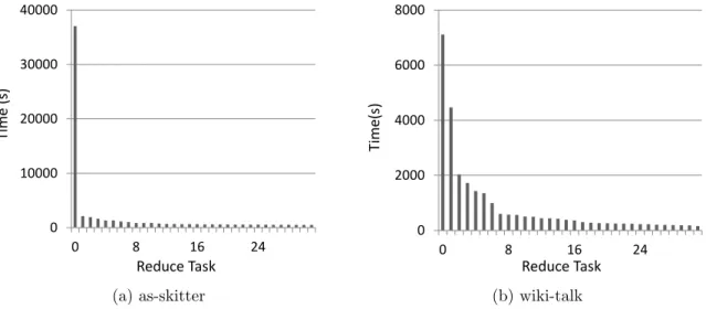
To understand the load balancing issue better, we implemented the na¨ıve algorithm (mod-ified to address problem (1)) and ran it on several graphs, recording the completion time of each reduce task. Figures 4.1 shows the completion time of each reduce task when the na¨ıve parallel algorithm is run on two different graphs. In each case, a single or small number of reduce tasks dominate the running time.
0 10000 20000 30000 40000 0 8 16 24 T im e ( s) Reduce Task (a) as-skitter 0 2000 4000 6000 8000 0 8 16 24 T im e (s ) Reduce Task (b) wiki-talk
Figure 4.1: Completion times of reduce tasks for the na¨ıve parallel algorithm, demonstrating poor load balancing. There is one bar for each of 32 reduce tasks, showing the time taken for the task.
4.3 Algorithm Enhancement
Without addressing the three problems discussed in the previous Section, the na¨ıve al-gorithm is unable to effectively take advantage of the parallelism provided by MapReduce. While removing duplicate cliques from the output is trivial, eliminating work redundancy and providing load balancing is not.
In MapReduce, there is no communication between reduce tasks, making dynamic solutions, such as dynamic load balancing or work stealing, impractical. These solutions would need to save the current state of each task to the file system and launch a new MapReduce job to redistribute work. Thus, it is worth investigating other avenues to reduce work redundancy and provide load balancing within the framework and algorithm.
In order to avoid work redundancy, we can assign a rank to each vertex in the graph. Using the vertex rank in combination with modifying the sets passed to the TTT algorithm (specifically by adding vertices with smaller rank to the Fini set), we can reduce the work redundancy down to an acceptable level by ignoring search paths that involve the vertices with smaller rank. To ensure the problem of duplicate results is still addressed, instead of enumerating a clique at the vertex with the smallest id, we only enumerate a clique C at the reduce task processing v∈C such that ∀u ∈C,rank(v) <rank(u). In other words, to avoid enumerating duplicate cliques, the vertex with the smallestrank in a clique is responsible for enumeration. Since there only exists a single vertex inCsatisfying this condition, it guarantees the clique will be output only once.
Furthermore, different strategies for assigning ranks to the vertices may be able to provide better load balancing by distributing the work across vertices. A vertex ordering defines how these ranks are assigned to the vertices of a graph. Ordering4.3.1and 4.3.2describe two such orderings.
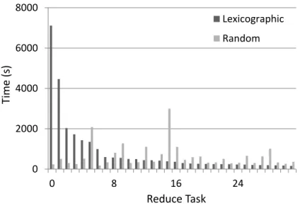
Figure 4.2demonstrates the impact of the two ordering strategies on the reduce task com-pletion times on the wiki-talk graph. The lexicographic ordering performs considerably worse than the random ordering. This poor performance is a result of an unfortunate labeling scheme of vertices in the input file such that a small vertex is a part of a large number of cliques,
demon-0 2000 4000 6000 8000 0 8 16 24 T im e ( s) Reduce Task Lexicographic Random
Figure 4.2: Comparison of reduce task running times when using the lexicographic and random ordering strategies on the wiki-talk graph.
strating that the different ordering schemes can improve load balance and motivating the search for better ordering schemes.
Ordering 4.3.1. Lexicographic Ordering
This is defined as rank(v) =v
Ordering 4.3.2. Random Ordering
This is defined as rank(v) = (r, v), where r is a random number between 0 and 1, and v is the vertex id. r is the most significant set of bits, withv only used in the event ther values of two vertices are equivalent.
An ideal ordering would balance the load successfully on an arbitrary graph. Intuitively, examining a vertex v ∈ V, the size of its subproblem is directly related to how many cliques it isresponsible for enumerating (the more cliques, the larger the subproblem), not how many cliques it is a part of. Therefore, if a vertex is in a large number of cliques, we would like it to come later in the ordering to reduce the number of these cliques it is responsible for enumerating. Therefore, a vertex v with a smaller rank than u is responsible for enumerating a larger portion of the cliques it is a part of. Overall, this increases the work done by smaller
vertices and decreases the work done by larger vertices, resulting in a more even distribution of work.
However, prior to running a clique enumeration algorithm it is not known how many cliques each vertex is contained in. Thus, a mechanism for approximating this ordering is used. Instead of ordering based on the number of cliques a vertex is a member of, the ordering uses the number of triangles a vertex is a member of. The intuition behind this is that if a vertex is a part of a large number of cliques, then it would be a part of a large number of triangles. Formally, the ordering proposed is defined as follows.
Ordering 4.3.3. Triangle Ordering
This is defined as rank(v) = (t, v), where t is the number of triangles the vertex is a part of, and v is the vertex id. t is the most significant set of bits, with v only used in the event the t
values of two vertices are equivalent.
The drawback to this approximation is that it will require a pre-processing step to count triangles. Counting triangles is a short and easy task compared to enumerating cliques, however since another MapReduce job is necessary, the overhead of this additional job needs to be taken into account.
This leads to a simpler, but less accurate approximation of the ordering by using the degree of a vertex. This information is contained inGv and therefore known to each reduce task. This
removes the need for a pre-processing step. The ordering can be formally defined as follows.
Ordering 4.3.4. Degree Ordering
This is defined as rank(v) = (d, v), where d = |Γ(v)|, and v is the vertex id. d is the most significant set of bits, with v only used in the event the dvalues of two vertices are equivalent.
In addition to removing work redundancy and providing load balancing, a well chosen vertex ordering scheme may also reduce the total work required by the algorithm when compared to na¨ıve ordering schemes. Eppstein et al. [11] investigated applying an ordering strategy to the sequential MCE problem. The reason for applying such an ordering scheme in the sequential problem is to limit the size of the subproblems rooted at each vertex in the graph and therefore
reduce the overall work. Thus, a well chosen ordering may reduce the subproblem sizes and consequently the total work in parallel MCE.
4.4 Parallel Enumeration of Cliques using Ordering
Parallel Enumeration of Cliques using Ordering (PECO) functions similar to the procedure described in Section4.1, however it applies the improvements discussed in Section4.3to reduce redundant work and balance the load. This section will discuss the details ofPECO.
The input to this algorithm is an undirected graphGstored as an adjacency list, such that if edge (w, u)∈E then the entry for wcontainsu, and likewise the entry for ucontains w.
Algorithm 2describes the mapfunction ofPECO. The function takes as input a single line of the adjacency list. From this it reads in a vertex v and Γ(v), and sends hv, Γ(v)i to each neighbor of v.
Algorithm 2:PECO Map(key,value)
Input: key- line number of input file
value- an adjacency list entry of the form hv, Γ(v)i
1 v← first vertex in value
2 Γ(v)← remaining vertices in value 3 for u∈Γ(v) do
4 emit(u,hv, Γ(v)i) 5 end
Algorithm 3 describes the reduce function of PECO. The reduce task for v receives as input the adjacency list entry for each u ∈ Γ(v). This allows the reduce task to create Gv.
Depending on the ordering selected, the ordering information will then be generated fromGv.
The reduce task creates the three sets needed to runTomita. K, the current (not necessarily maximal) clique to extend, begins as {v}. Cand is then Γ(v) andFini is empty. However, due to the vertex ordering this reduce task is only responsible for enumerating cliques where v is the smallest vertex according to the ordering. To avoid enumerating other cliques and reduce work redundancy, lines 6-11 do the important step of removing any vertex from Cand that is smaller than v and adding it to Fini. Recall, any clique that includes a vertex in Fini will not be enumerated by Tomita. After creating these three sets, Tomita is called with these
sets as input parameters. The cliques are emitted within the Tomita function as described in Section2.3.
Algorithm 3:PECO Reduce(v, list(value))
Input: v - enumerate cliques containing this vertex
list(value) - adjacency list entries for eachu∈Γ(v) 1 Gv ← induced subgraph on vertex set v∪Γ(v)
2 rank← generated according to ordering selected 3 K ← {v}
4 Cand←Γ(v) 5 Fini← { }
6 for u∈Γ(v) do
7 if rank(u)<rank(v) then
8 Cand←Cand− {u}
9 Fini←Fini∪ {u}
10 end
11 end
12 Tomita(Gv, K,Cand,Fini)
4.5 Correctness of PECO
To prove the correctness of PECO, the correctness of the map and reduce functions must be shown.
Claim 4.5.1. The PECO map function (algorithm 2) correctly sends Gv to Rv, where Rv is the reduce task processing vertex v.
Proof. Themapfunction is called once for each line of the adjacency list. Consider the adjacency entry for v. Line 4 sends to each u∈Γ(v) the adjacency list entry for v.
Now consider Rv. It will receive an adjacency list entry for each u∈Γ(v). From this, v is
able to determine Γ(v), as well as Γ(u) for eachu∈Γ(v) to createGv.
Claim 4.5.2. For a given v and Gv, the PECO reduce function (algorithm 3) correctly enu-merates all cliques which (1) v is a part of in G and (2) v is the smallest vertex with respect to the ordering.
Proof. Assume Gv and a vertex ordering are correctly received as input by Claim 4.5.1. Let
ζ be the set of all maximal cliques in G. Examine C ∈ζ and assume v is the smallest vertex in C with respect to the ordering. Now consider Rv. The if statement in line 7 will never
evaluate to true foru∈C sincev is the smallest vertex inC. Thus, every vertex in C will be in the Cand set when the call to Tomita is made. As a result, v will enumerate C. Overall, v will enumerate eachC ∈ζ wherev is the smallest vertex.
Claim 4.5.3. The MapReduce algorithm PECO (1) Enumerates all maximal cliques in G. (2) Does not output the same clique more than once. (3) Outputs no non-maximal cliques.
Proof. (1) Letζ be the set of all maximal cliques in Gand examineC∈ζ. By the correctness of the PECO reduce function, each clique will be enumerated by the smallest vertex in C. This shows that eachC ∈ζ will be enumerated at a vertex, and across all vertices the entire set ζ will be enumerated.
(2) Now consider the reduce task processing a vertex y∈C− {x}, where x is the smallest vertex inC. Theif statement in line 7 of the reduce function will evaluate to be true at least once, asrank(x)<rank(y). Thus,xwill be removed from theCand set and added to theFini set. WhenTomitais executed, cliqueC will not be enumerated aty, since x∈Fini. Thus, no duplicate cliques will be enumerated by the algorithm.
(3) The reduce task for v has Gv, the subgraph induced by {v} ∪ Γ(v). Every cliuqe
enumerated byRv must containv by line 3 of thePECO reducefunction, and any clique inG
which containsv, is completely contained withinGv. Therefore, when Gv is passed to Tomita,
TTT guarantees only maximal cliques will be enumerated.
4.6 PECO and Other Parallel Frameworks
Now that the PECO algorithm has been explained in full. We will briefly discuss imple-mentingPECO on other parallel frameworks.
4.6.1 Pregel
The PECO algorithm can be easily adapted to fit Pregel [30]. In the first superstep, each vertex sends its neighborhood to each neighbor. In the second superstep, each vertex now has the subgraph Gv and can locally calculate the maximal cliques it is a part of, enumerating
cliques in which it is the smallest vertex with respect to an ordering. Although this translation to Pregel is possible, current open source implementation of the Pregel framework are in their early stages, and are not ready for evaluation. Furthermore, PECO was designed for a com-munication restricted framework, where Pregel allows for comcom-munication oriented algorithms. This may allow further load balancing improvements to be made to the algorithm. For exam-ple, each vertex may only process its subgraph for a period of time before pausing execution. Vertices which have finished their work can then request additional work from neighbors in order to avoid sitting idle.
4.6.2 Dryad
Translating PECO into the Dryad [19] framework may simply require writing the map and reduce functions as individual programs and correctly defining the Dryad job graph. The job graph would most likely be a very simple graph as there would only exist map and reduce vertices in this graph. However, as this system is not as widely used as other parallel frameworks, the authors did not investigate implementation details further.
4.6.3 MPI
PECO can be implemented as a relatively simple MPI [38] program. However, MPI allows for more generic communication schemes then PECO uses. This allows for more complex algorithms to be written, which can take advantage of dynamic load balancing techniques not available in MapReduce, such as in [37]. On the other hand, the algorithm in [37] cannot be translated into an efficient MapReduce algorithm. Furthermore, an MPIPECOimplementation would need to manually handle fault tolerance.
CHAPTER 5. RESULTS
All reported experiments were run on the Hadoop [1, 41] cluster at the Cloud Computing Testbed located at the University of Illinois Urbana-Champaign. The cluster consists of 62 HP DL160 compute nodes each with dual quad core CPUs, 16GB of RAM, and 2TB disk space. 372 of the cluster cores are configured to run map tasks, while the remaining 124 cores are configured to run reduce tasks.
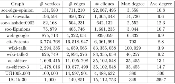
Experiments are run on graphs from the Stanford large graph database [23], as well as on Erd¨os-R´enyi random graphs. The test graphs used are given in Table5.1 along with some basic properties. The soc-sign-epinion[24], soc-epinion[35], loc-gowalla[7], and soc-slashdot0902 [26] graphs represent typical social networks, where vertices represent users and edges represent friendships. cit-patents [15] is a citation graph for U.S. patents granted between 1975 and 1999. In the wiki-talk graph [24] vertices represent users and edges represent edits to other users’ talk pages. web-google [26] is web graph with pages represented by vertices and hyperlinks by edges. The as-skitter graph [25] is an internet routing topology graph collected from a year of daily traceroutes. For the purpose of clique enumeration, these graphs are all treated as undirected. The wiki-talk-3 and as-skitter-3 graphs are the wiki-talk and as-skitter graphs, respectively, with all vertices of degree less than or equal to 2 removed. Two random graphs are also used in the experiments. UG100k.003 is a random graph with 100,000 vertices and a probability of 0.003 of an edge being present, while UG1k.3 has 1,000 vertices and a probability of 0.3.
Graph # vertices # edges # cliques Max degree Ave degree soc-sign-epinion 131,580 711,210 22,067,495 3,558 10.8 loc-Gowalla 196,591 950,327 1,005,048 14,730 9.6 soc-slashdot0902 82,168 504,231 642,132 2,552 12.3 soc-Epinions 75,879 405,746 1,681,235 3,044 10.7 web-google 875,713 4,322,051 939,059 6,332 9.9 cit-Patents 3,774,768 16,518,947 6,061,991 793 8.8 wiki-talk 2,294,385 4,659,565 83,355,058 100,029 3.9 wiki-talk-3 626,749 2,894,276 83,355,058 46,257 9.2 as-skitter 1,696,415 11,095,298 35,102,548 35,455 13.1 as-skitter-3 1,478,016 10,877,499 35,102,548 35,455 14.7 UG100k.003 100,000 14,997,901 4,488,632 380 300 UG1k.30 1,000 149,851 15,112,753 349 299.7
Table 5.1: Graph statistics.
5.1 Ordering Strategy Evaluation
5.1.1 Strategy comparison
In order to compare the different ordering strategies, each was run on the set of test graphs. To limit the focus to the impact each strategy has, the running time of just the reduce tasks is examined. This ignores the map and shuffle phases. The different strategies do not vary in their map functions and limiting the focus to only the reduce task will remove the impact of network traffic on the running times. Table 5.2 shows the completion time of the longest running reduce task for each graph and ordering strategy.
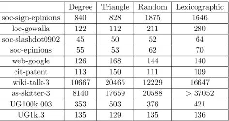
It is clear from the table that the degree and triangle orderings are superior to the other two strategies when only considering the running times of the reduce tasks. This is particularly evident on the more challenging graphs such as soc-sign-epinions, wiki-talk-3, and as-skitter-3 where these orderings see a reduction in time of over 50% when compared to the random or lexicographic orderings. However, the previous table (Table5.2) ignored the triangle counting pre-processing step, which needs to be considered to ensure this step is not too time consuming. Table5.3 shows the total running time (i.e. the time for map, shuffle, and reduce phases) for each ordering strategy.
Degree Triangle Random Lexicographic soc-sign-epinions 800 784 1843 1615 loc-gowalla 36 29 45 130 soc-slashdot0902 16 16 23 32 soc-epinions 25 21 32 41 web-google 70 65 86 79 cit-patent 64 59 64 63 wiki-talk-3 823 610 2999 7113 as-skitter-3 2091 2326 14009 >37052 UG100k.003 226 223 238 269 UG1k.3 103 101 98 107
Table 5.2: Completion time (seconds) of the longest reduce task for the combinations of graphs and ordering strategies.
Degree Triangle Random Lexicographic
soc-sign-epinions 840 828 1875 1646 loc-gowalla 122 112 211 280 soc-slashdot0902 45 50 52 64 soc-epinions 55 53 62 70 web-google 126 168 144 140 cit-patent 113 150 111 109 wiki-talk-3 10667 20465 12229 16647 as-skitter-3 8140 17659 20588 >37052 UG100k.003 353 503 376 421 UG1k.3 135 129 135 136
Table 5.3: Total running times (seconds) for all the combinations of graphs and ordering strategies.
well as the degree ordering. This is most evident in the wiki-talk-3 and as-skitter-3 completion times, where the map and shuffle phase contribute to a large portion of the total time. Since the triangle ordering requires two MapReduce jobs, this portion of the overall doubles. As a result, the degree ordering sees the lowest total running times.
5.1.2 Load balancing versus enumeration time reduction
The degree ordering strategy sees a significant decrease in running time when compared to the other strategies. However, it is not clear if this reduction in running time is due to superior load balancing, or an improvement in the enumeration time, or a combination of both.
Figure 5.1 motivates this inquiry further. The figure shows the reduce task completion times for the degree ordering and lexicographic ordering on the soc-sign-epinion and loc-gowalla graphs. The degree ordering has a smaller overall running time; however it is difficult to tell what impact load balancing or reduced enumeration time have on this.
0 600 1200 1800 1 2 3 4 5 6 7 8 T im e ( s) Reduce Task Lexicographic Degree (a) soc-sign-epinion 0 30 60 90 120 150 1 2 3 4 5 6 7 8 T im e ( s) Reduce Task Lexicographic Degree (b) loc-gowalla
Figure 5.1: A comparison of reduce task completion times between the lexicographic ordering and degree ordering on the soc-sign-epinion and loc-gowalla graphs.
To evaluate which of these two factors is contributing to the reduction, the following mea-sures are proposed to evaluate each. The sum of the individual reduce task running times will be used to determine if a reduction in enumeration time has occurred. More formally, let
T(order) = #Tasks
X
i=1
ti (5.1)
where ti is the ”work” of reducer i and T is the total work of all reducers. When comparing
two ordering strategies, if there is no change in enumeration time between the two strategies, thenT(order1) =T(order2).
Measuring load balancing is more challenging. The first step is to normalize the reduce task running times to determine the proportion of the overall work each task is responsible for. For reduce task i, letPi(order) represent the proportion of overall work i is responsible for when
applying orderingorder. Then,
Pi(order) =
ti
P(order) ={Pi(order)} 0≤i <# tasks (5.3)
Then, the load balance of an ordering can be measured by the standard deviation ofP(order). Let, L(order) be the load balance of an ordering, defined by equation 5.4.
L(order) =stdev(P(order)) (5.4)
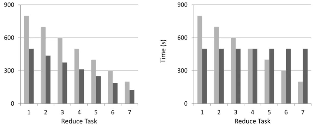
Thus, two orderings may have different running times, but have the same load balance. Fig-ure 5.2a illustrate two such orderings and figure 5.2b depicts two orderings where there is no difference in enumeration time but the load balance has changed.
0 300 600 900 1 2 3 4 5 6 7 T im e ( s) Reduce Task
(a) Two orderings with equal load balance.
0 300 600 900 1 2 3 4 5 6 7 T im e ( s) Reduce Task
(b) Two orderings with equal enumeration time. Figure 5.2: (a) shows a comparison of two ordering strategies with equal load balance. (b) shows a comparison of two ordering strategies with equal enumeration time.
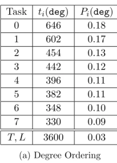
Table5.3showsT andLfor the degree and lexicographic orderings on the soc-sign-epinions graph. Comparing T(deg) andT(lex), it is evident that there is a reduction in enumeration time from lexicographic to degree. Similarly, the degree ordering has a smaller L value than lexicographic, indicating a better load balance. However, from these tables alone it is not possible to determine if these differences are significant.
In order to determine if the differences are statistically significant, the following test was applied. The two strategies were each run five times on the soc-sign-epinions graph, collecting T and Lfrom each trial. µT(deg),σT(deg),µL(deg),σL(deg),µT(lex),σT(lex),µL(lex), and σL(lex),
Task ti(deg) Pi(deg) 0 646 0.18 1 602 0.17 2 454 0.13 3 442 0.12 4 396 0.11 5 382 0.11 6 348 0.10 7 330 0.09 T, L 3600 0.03 (a) Degree Ordering
Task ti(lex) Pi(lex)
0 1210 0.20 1 1081 0.17 2 1010 0.16 3 940 0.15 4 730 0.12 5 643 0.10 6 387 0.16 7 180 0.03 T, L 6181 0.05 (b) Lexicographic Ordering
Figure 5.3: Load balancing and time reduction statistics for the soc-sign-epinions graph.
were calculated, were µX is the mean of the corresponding measure and σX is the standard
deviation. Equation5.5 gives the null hypotheses.
H0 :µT(deg)=µT(lex)
H0:µL(deg)=µL(lex)
(5.5)
Equation 5.6gives the alternative hypotheses.
Ha:µT(deg)< µT(lex)
Ha:µL(deg)< µL(lex)
(5.6)
The test statistic is given by Equation5.7.
Z = rxdeg¯ −xlex¯ s2 deg ndeg + s2 lex nlex (5.7)
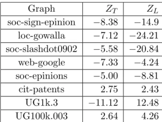
Values of Z <−2 represent strong evidence to reject the null hypothesis in favor of the alter-native. This test was repeated for each available test graph (excluding wiki-talk, as-skitter) with the result summarized in Table5.4.
Overall, on real graphs the degree ordering improves both load balance and enumeration time when compared to the lexicographic ordering. On cit-patents and UG100k.003, the evi-dence does not support an improvement of these factors, and on UG1k.3 an improvement in enumeration time is seen, but not in load balancing.
As previously mentioned, Eppstein et al. [11] applied an ordering strategy in a sequential enumeration algorithm. Eppsteinet al. parameterize the MCE problem with respect to graph
Graph ZT ZL soc-sign-epinion −8.38 −14.9 loc-gowalla −7.12 −24.21 soc-slashdot0902 −5.58 −20.84 web-google −7.33 −4.24 soc-epinions −5.00 −8.81 cit-patents 2.75 2.43 UG1k.3 −11.12 12.48 UG100k.003 2.64 4.26
Table 5.4: Hypothesis test comparing the degree ordering and lexicographic ordering.
degeneracy. They show that by processing vertices in the degeneracy ordering, their algorithm can achieve faster running times than Tomitaet al. [39] or perform only a constant factor worse. The degeneracy ordering of a graph is dependent on the degrees of the vertices. We believe that the degree ordering used inPECOis approximating the degeneracy ordering. Approximation of degeneracy orderings has not been previously studied because generating the order sequentially can be done trivially in O(nm) time. However, in the MapReduce framework it is not clear how to efficiently produce this ordering. Even if we could, it would result in additional rounds of Mapreduce, and may not help overall.
5.2 PECO Scalability
An important measure for any parallel algorithm is to determine how well is scales to larger numbers of processors. PECO is run on several graphs using 1, 2, 4, 8, 16, 32, and 64 reduce tasks. Figure5.4a and5.4c show the speedup of just the reduce tasks on the soc-sign-epinions and web-google graphs, respectively. Both graphs show good speedup, with the web-google graph achieving a speedup up of 42 on 64 reduce tasks. Figure5.4band5.4dshow the speedup for the two graphs when considering the entire job time. The soc-sign-epinions graph sees little change from the reduce task only graph, as communication costs contribute little to the overall running time. However, the web-google graph sees a larger impact, as the communication cost makes up a larger portion of the total run time.
1 2 4 8 16 32 64 1 2 4 8 16 32 64 S p e e d u p # of Reduce Tasks Degree Triangle Ideal
(a) soc-sign-epinion reduce task speedup
1 2 4 8 16 32 64 1 2 4 8 16 32 64 S p e e d u p # of Reduce Tasks Degree Triangle Ideal
(b) soc-sign-epinion overall speedup
1 2 4 8 16 32 64 1 2 4 8 16 32 64 S p e e d u p # of Reduce Tasks Degree Triangle Ideal
(c) web-google reduce task speedup
1 2 4 8 16 32 64 1 2 4 8 16 32 64 S p e e d u p # of Reduce Tasks Degree Triangle Ideal
(d) web-google overall speedup Figure 5.4: PECO scalability for the degree and triangle ordering strategies.
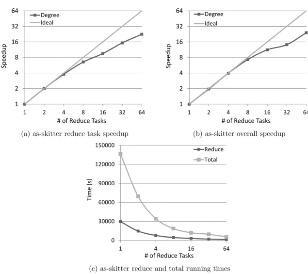
as-skitter graph. In order to better examine the scalability of both the communication and enumeration aspects of the algorithm, the speedup of the degree ordering is examined on the as-skitter-3 graph. Figure 5.5a shows the speedup of just the reduce tasks. A speedup of 22 with 64 reduce tasks is achieved. When the running time of the entire job is considered (Figure 5.5b), the speedup increases slightly to 24, demonstrating that the communication aspect of the algorithm scales well on large graphs. Figure5.5ccompares the completion times of the reduce phase to those of the overall running time.
1 2 4 8 16 32 64 1 2 4 8 16 32 64 S p e e d u p # of Reduce Tasks Degree Ideal
(a) as-skitter reduce task speedup
1 2 4 8 16 32 64 1 2 4 8 16 32 64 S p e e d u p # of Reduce Tasks Degree Ideal
(b) as-skitter overall speedup
0 30000 60000 90000 120000 150000 1 4 16 64 T im e ( s) # of Reduce Tasks Reduce Total
(c) as-skitter reduce and total running times Figure 5.5: PECO large graph scalability
5.3 Summary and Comparison to Other Algorithms
Table 5.5 gives a summary of the degree ordering running times on the test graphs. The final column gives available results of the dMaximalClique algorithm. This column is the sum of the enumeration and filtering times as listed in Table III of [27].
It is difficult to make detailed comparisons to the dMaximalCliques algorithm due to differ-ences is hardware and lack of implementation details on dMaximalCliques. However, directly comparing the Total columns for each algorithm provides evidence that PECO could be sub-stantially faster than dMaximalCliques, particularly on the larger graphs. Furthermore, [27] does not discuss communication times of dMaximalCliques; thus, the difference in running
Graph # reduce tasks Comm. time Enum. time Total dMC Total
soc-sign-epinion 8 40 sec 13.3 min 14 min NA
loc-gowalla 8 1.4 min 36 sec 2 min NA
soc-slashdot0902 8 29 sec 16 sec 45 sec NA
soc-epinion 8 30 sec 25 sec 55 sec 3.2 min
web-google 8 56 sec 1.2 min 2.1 min 56 sec
cit-patents 8 49 sec 1.1 min 1.9 min 6.42 min
wiki-talk-3 32 164 min 14 min 178 min 235 min
as-skitter-3 32 101 min 35 min 136 min 194 min
UG1k.3 8 32 sec 1.7 min 2.25 min NA
UG100k.003 16 2.1 min 3.8 min 5.9 min NA
Table 5.5: Summary of results for degree ordering on available test graphs. For reference the total time for dMaximalCliques is entered as dMC Total, as reported in [27]. This total does not include communication times.
CHAPTER 6. CONCLUSION
MCE is a important problem in graph theory with many practical applications. As a result, sequential enumeration algorithms have been heavily studied. However, as graph sizes have continued to increase, reaching millions of vertices and edges, a need for parallel algorithms has arose.
This work presented a novel parallel algorithm, PECO, for enumerating maximal cliques in large graphs. Inducing a strict ordering over the vertices and using this in conjunction with a sequential MCE algorithm, PECO reduces redundant work and only enumerates a clique contained in a subgraph if the clique satisfies a certain condition with respect to the ordering, ensuring that each maximal clique is output exactly once. The vertex ordering also greatly improves load balancing when compared with straightforward approaches to parallelization. Previous works require post-processing steps to remove duplicate and non-maximal cliques, and do not address the issue of load balancing. Furthermore, a well chosen vertex ordering can reduce the size of the subproblems and therefore reduce overall enumeration time when compared to na¨ıve ordering schemes.
Experiments performed on large real world graphs demonstrate that PECOcan enumerate cliques in graphs with millions of edges and scales well to at least 64 processors. A comparison of ordering strategies showed that an ordering based on vertex degree performs the best, reducing both enumeration time and improving load balancing.
BIBLIOGRAPHY
[1] Hadoop. http://hadoop.apache.org/. Accessed on 10 January 2012. Project homepage. [2] C. Bron and J. Kerbosch. Algorithm 457: finding all cliques of an undirected graph.
Commun. ACM, 16:575–577, September 1973.
[3] F. Cazals and C. Karande. A note on the problem of reporting maximal cliques.Theoretical Computer Science, 407(1-3):564 – 568, 2008.
[4] Y. Chen and G. M. Crippen. A novel approach to structural alignment using realistic structural and environmental information. Protein Science, 14(12):2935–2946, 2005. [5] J. Cheng, Y. Ke, A. W.-C. Fu, J. X. Yu, and L. Zhu. Finding maximal cliques in massive
networks by h*-graph. InProceedings of the 2010 international conference on Management of data, SIGMOD ’10, pages 447–458, New York, NY, USA, 2010. ACM.
[6] N. Chiba and T. Nishizeki. Arboricity and subgraph listing algorithms.SIAM J. Comput., 14:210–223, February 1985.
[7] E. Cho, S. A. Myers, and J. Leskovec. Friendship and mobility: user movement in location-based social networks. InProceedings of the 17th ACM SIGKDD international conference on Knowledge discovery and data mining, KDD ’11, pages 1082–1090, New York, NY, USA, 2011. ACM.
[8] J. Dean and S. Ghemawat. Mapreduce: simplified data processing on large clusters. In
Proceedings of the 6th conference on Symposium on Opearting Systems Design & Imple-mentation - Volume 6, pages 10–10, Berkeley, CA, USA, 2004. USENIX Association.
[9] N. Du, B. Wu, L. Xu, B. Wang, and X. Pei. A parallel algorithm for enumerating all maximal cliques in complex network. InData Mining Workshops, 2006. ICDM Workshops 2006. Sixth IEEE International Conference on, pages 320 –324, dec. 2006.
[10] J. L. E. Lawler and A. R. Kan. Generating all maximal independent sets: Np-hardness and polynomial-time algorithms. SIAM Journal of Computing, 9, August 1980.
[11] D. Eppstein, M. Lffler, and D. Strash. Listing all maximal cliques in sparse graphs in near-optimal time. In O. Cheong, K.-Y. Chwa, and K. Park, editors, Algorithms and Computation, volume 6506 ofLecture Notes in Computer Science, pages 403–414. Springer Berlin / Heidelberg, 2010.
[12] D. Eppstein and D. Strash. Listing all maximal cliques in large sparse real-world graphs. In P. Pardalos and S. Rebennack, editors, Experimental Algorithms, volume 6630 ofLecture Notes in Computer Science, pages 364–375. Springer Berlin / Heidelberg, 2011.
[13] H. M. Grindley, P. J. Artymiuk, D. W. Rice, and P. Willett. Identification of tertiary struc-ture resemblance in proteins using a maximal common subgraph isomorphism algorithm.
Journal of Molecular Biology, 229(3):707 – 721, 1993.
[14] Y. Gu and R. L. Grossman. Sector and sphere: the design and implementation of a high-performance data cloud.Philosophical Transactions of the Royal Society A: Mathematical, Physical and Engineering Sciences, 367(1897):2429–2445, 2009.
[15] B. H. Hall, A. B. Jaffe, and M. Trajtenberg. The nber patent citation data file: Lessons, insights and methodological tools. NBER Working Papers 8498, National Bureau of Eco-nomic Research, Inc, Oct 2001.
[16] E. Harley and A. Bonner. Uniform integration of genome mapping data using intersection graphs. Bioinformatics, 17(6):487–494, 2001.
[17] M. Hattori, Y. Okuno, S. Goto, and M. Kanehisa. Development of a chemical structure comparison method for integrated analysis of chemical and genomic information in the
metabolic pathways. Journal of the American Chemical Society, 125(39):11853–11865, 2003.
[18] Ina and Koch. Enumerating all connected maximal common subgraphs in two graphs.
Theoretical Computer Science, 250(1-2):1 – 30, 2001.
[19] M. Isard, M. Budiu, Y. Yu, A. Birrell, and D. Fetterly. Dryad: distributed data-parallel programs from sequential building blocks. SIGOPS Oper. Syst. Rev., 41(3):59–72, Mar. 2007.
[20] D. S. Johnson, M. Yannakakis, and C. H. Papadimitriou. On generating all maximal independent sets. Information Processing Letters, 27(3):119 – 123, 1988.
[21] P. F. Jonsson and P. A. Bates. Global topological features of cancer proteins in the human interactome. Bioinformatics, 22(18):2291–2297, 2006.
[22] F. Kose, W. Weckwerth, T. Linke, and O. Fiehn. Visualizing plant metabolomic correlation networks using clique-metabolite matrices. Bioinformatics, 17(12):1198–1208, 2001. [23] J. Leskovec. Stanford large network dataset collection. http://snap.stanford.edu/
data/index.html. Accessed 4 June 2012. Downloaded soc-Epinions1.txt.gz, Slash-dot0902.txt.gz, Wiki-Talk.txt.gz, cit-Patents.txt.gz, web-Google.txt.gz, as-skitter.txt.gz, soc-sign-epinions.txt.gz, and loc-gowalla edges.txt.gz.
[24] J. Leskovec, D. Huttenlocher, and J. Kleinberg. Signed networks in social media. In
Proceedings of the 28th international conference on Human factors in computing systems, CHI ’10, pages 1361–1370, New York, NY, USA, 2010. ACM.
[25] J. Leskovec, J. Kleinberg, and C. Faloutsos. Graphs over time: densification laws, shrink-ing diameters and possible explanations. In Proceedings of the eleventh ACM SIGKDD international conference on Knowledge discovery in data mining, KDD ’05, pages 177–187, New York, NY, USA, 2005. ACM.
[26] J. Leskovec, K. J. Lang, A. Dasgupta, and M. W. Mahoney. Community structure in large networks: Natural cluster sizes and the absence of large well-defined clusters. Internet Mathematics, 6(1):29–123, 2009.
[27] L. Lu, Y. Gu, and R. Grossman. dmaximalcliques: A distributed algorithm for enumer-ating all maximal cliques and maximal clique distribution. In Data Mining Workshops (ICDMW), 2010 IEEE International Conference on, pages 1320 –1327, dec. 2010.
[28] M. O. M. J. Zaki, S. Parthasarathy and W. Li. New algorithms for fast discovery of association rules. InIn 3rd Intl. Conf. on Knowledge Discovery and Data Mining, pages 283–286. AAAI Press, 1997.
[29] K. Makino and T. Uno. New algorithms for enumerating all maximal cliques. In T. Hagerup and J. Katajainen, editors,Algorithm Theory - SWAT 2004, volume 3111 ofLecture Notes in Computer Science, pages 260–272. Springer Berlin / Heidelberg, 2004.
[30] G. Malewicz, M. H. Austern, A. J. Bik, J. C. Dehnert, I. Horn, N. Leiser, and G. Cza-jkowski. Pregel: a system for large-scale graph processing - ”abstract”. InProceedings of the 28th ACM symposium on Principles of distributed computing, PODC ’09, pages 6–6, New York, NY, USA, 2009. ACM.
[31] N. Modani and K. Dey. Large maximal cliques enumeration in sparse graphs. In Proceed-ings of the 17th ACM conference on Information and knowledge management, CIKM ’08, pages 1377–1378, New York, NY, USA, 2008. ACM.
[32] S. Mohseni-Zadeh, P. Brzellec, and J.-L. Risler. Cluster-c, an algorithm for the large-scale clustering of protein sequences based on the extraction of maximal cliques. Computational Biology and Chemistry, 28(3):211 – 218, 2004.
[33] J. Moon and L. Moser. On cliques in graphs. Israel Journal of Mathematics, 3:23–28, 1965. 10.1007/BF02760024.
[34] G. Palla, I. Dernyi, I. Farkas, and T. Vicsek. Uncovering the overlapping community structure of complex networks in nature and society. Nature, 435(7043):814 – 818, 2005.
[35] M. Richardson, R. Agrawal, and P. Domingos. Trust management for the semantic web. In D. Fensel, K. Sycara, and J. Mylopoulos, editors,The Semantic Web - ISWC 2003, volume 2870 ofLecture Notes in Computer Science, pages 351–368. Springer Berlin / Heidelberg, 2003.
[36] O. Rokhlenko, Y. Wexler, and Z. Yakhini. Similarities and differences of gene expression in yeast stress conditions. Bioinformatics, 23(2):e184–e190, 2007.
[37] M. C. Schmidt, N. F. Samatova, K. Thomas, and B.-H. Park. A scalable, parallel algorithm for maximal clique enumeration. J. Parallel Distrib. Comput., 69:417–428, April 2009. [38] M. Snir, S. W. Otto, D. W. Walker, J. Dongarra, and S. Huss-Lederman. MPI: The
Complete Reference. MIT Press, Cambridge, MA, USA, 1995.
[39] E. Tomita, A. Tanaka, and H. Takahashi. The worst-case time complexity for generating all maximal cliques and computational experiments. Theor. Comput. Sci., 363:28–42, October 2006.
[40] S. Tsukiyama, M. Ide, H. Ariyoshi, and I. Shirakawa. A new algorithm for generating all the maximal independent sets. SIAM J. Comput., 6(3):505–517, 1977.
[41] T. White. Hadoop: The Definitive Guide. O’Reilly Media, Inc., 2010.
[42] B. Wu, S. Yang, H. Zhao, and B. Wang. A distributed algorithm to enumerate all maximal cliques in mapreduce. InFrontier of Computer Science and Technology, 2009. FCST ’09. Fourth International Conference on, pages 45 –51, dec. 2009.
[43] B. Zhang, B.-H. Park, T. Karpinets, and N. F. Samatova. From pull-down data to protein interaction networks and complexes with biological relevance. Bioinformatics, 24(7):979– 986, 2008.
[44] Y. Zhang, F. Abu-Khzam, N. Baldwin, E. Chesler, M. Langston, and N. Samatova. Genome-scale computational approaches to memory-intensive applications in systems bi-ology. In Supercomputing, 2005. Proceedings of the ACM/IEEE SC 2005 Conference, page 12, nov. 2005.