Analysing sequencing data in Hadoop: The road to interactivity via SQL

(1)

Aalto University School of Science

Degree Programme of Computer Science and Engineering

Matti Niemenmaa

Analysing sequencing data in Hadoop:

The road to interactivity via SQL

Master’s Thesis

Espoo, 16th November 2013

Supervisor: Assoc. Prof. Keijo Heljanko Advisor: Assoc. Prof. Keijo Heljanko

(2)

(3)

Aalto University School of Science

Degree Programme of Computer Science and Engineering

ABSTRACT OF MASTER’S THESIS Author: Matti Niemenmaa

Title:

Analysing sequencing data in Hadoop: The road to interactivity via SQL

Date: 16th November 2013 Pages: xv+143

Major: Theoretical Computer Science Code: T-79 Supervisor: Assoc. Prof. Keijo Heljanko

Advisor: Assoc. Prof. Keijo Heljanko

Analysis of high volumes of data has always been performed with distributed comput-ing on computer clusters. But due to rapidly increascomput-ing data amounts in, for example, DNA sequencing, new approaches to data analysis are needed. Warehouse-scale computing environments with up to tens of thousands of networked nodes may be necessary to solve future Big Data problems related to sequencing data analysis. And to utilize such systems eﬀectively, specialized software is needed.

Hadoop is a collection of software built speciﬁcally for Big Data processing, with a core consisting of the Hadoop MapReduce scalable distributed computing platform and the Hadoop Distributed File System, HDFS. This work explains the principles underlying Hadoop MapReduce and HDFS as well as certain prominent higher-level interfaces to them: Pig, Hive, and HBase. An overview of the current state of Hadoop usage in bioinformatics is then provided alongside brief introductions to the Hadoop-BAM and SeqPig projects of the author and his colleagues.

Data analysis tasks are often performed interactively, exploring the data sets at hand in order to familiarize oneself with them in preparation for well targeted long-running computations. Hadoop MapReduce is optimized for throughput instead of latency, making it a poor ﬁt for interactive use. This Thesis presents two high-level alternatives designed especially with interactive data analysis in mind: Shark and Impala, both of which are Hive-compatible SQL-based systems.

Aside from the computational framework used, the format in which the data sets are stored can greatly aﬀect analytical performance. Thus new ﬁle formats are being developed to better cope with the needs of modern and future Big Data sets. This work analyses the current state of the art storage formats used in the worlds of bioinformatics and Hadoop.

Finally, this Thesis presents the results of experiments performed by the author with the goal of understanding how well the landscape of available frameworks and storage formats can tackle interactive sequencing data analysis tasks.

Keywords: Hive, Shark, Impala, Hadoop, MapReduce, HDFS, SQL, sequencing data, Big Data, interactive analysis

(4)

(5)

Acknowledgements

To my supervisor and my colleagues at work, for the valuable feedback on the content of this Thesis and for teaching me some things I needed to know.

To my friends at Aalto, for the stimulating lunchtime discussions. To my family and girlfriend, for your support and patience.

Espoo, 16th November 2013

(6)

(7)

List of abbreviations

Throughout this work, abyte represents an eight-bit quantity. API application programming interface

BAM Binary Alignment/Map [Li+09; SAM13]

bp base pair

BCF Binary Call Format [Dan+11] BED Browser Extensible Data [Qui+10]

BGZF Blocked GNU Zip Format(according to e.g. Cánovas and Moﬀat [Cán+13] and Cock [Coc11])

BGI 华大基因, a Chinese genomics research institute; formerly

Beijing Genomics Institute

CDH Cloudera’s Distribution Including Apache Hadoop [CDH] CIGAR Compact Idiosyncratic Gapped Alignment Report [Ens13] CPU central processing unit

CRC cyclic redundancy check [Pet+61] DAG directed acyclic graph

DDR3 double data rate [DDR08], type three

DEFLATE a compressed data format, or the canonical compression algorithm outputting data in that format [Deu96a]

DistCp distributed copy, a ﬁle copying tool using Hadoop Map-reduce[DCp]

DNA deoxyribonucleic acid

DOI Digital Object Identiﬁer [DOI] ETL Extract, Transform, and Load

GATK the Genome Analysis Toolkit [McK+10] GB gigabytes (109_bytes)

Gbps gigabits per second (109_{bits per second)} GFS the Google File System [Ghe+03]

(10)

L  

GHz gigahertz (109_Hertz) GiB gibibytes (230_bytes)

GNU GNU’s Not Unix! [GNU]

HDFS the Hadoop Distributed File System

HiveQL the Hive query language(in this work, also used to refer to the dialects understood by Shark and Impala)

HTS high-throughput sequencing

I/O input/output

JBOD just a bunch of disks

JVM Java Virtual Machine

kB kilobytes (103_bytes) KiB kibibytes (210_bytes)

LLVM a collection of compiler-related software projects [LLV]; formerly Low-Level Virtual Machine [Lat+04]

LZMA Lempel-Ziv-Markov chain algorithm [Pav13] LZO Lempel-Ziv-Oberhumer [Obe]

MB megabytes (106_bytes) MHz megahertz (106_Hertz) MiB mebibytes (220_bytes)

Mibp mebi-base pairs (220_{base pairs)} MPI Message Passing Interface [MPI93] MTBF mean time between failures

N/A not applicable

NFS Network File System [Sto+10] NGS next-generation sequencing

ORC Optimized Row Columnar [ORC13; ORM] PB petabytes (1015_bytes)

PiB pebibytes (250 _bytes)

PNG Portable Network Graphics [Duc03]

QC quality control

QDR quad data rate

RAM random access memory

RCFile Record Columnar File [He+11]

RDD Resilient Distributed Dataset [Zah+12] RPM revolutions per minute

SAM Sequence Alignment/Map [Li+09; SAM13]

SDRAM synchronous dynamic random access memory [SDR94] SerDe serializer/deserializer

SQL Structured Query Language [ISO92] SSTable Sorted String Table [McK+09] stddev standard deviation

(11)

TB terabytes (1012_bytes) TiB tebibytes (240 _bytes)

URL Uniform Resource Locator [Ber+05] UTF Unicode Transformation Format [UTF] VCF Variant Call Format [Dan+11]

XML Extensible Markup Language [Bra+08] YARN Yet Another Resource Negotiator [Wat12]

(12)

(13)

List of Tables

6.1 BCF record format. . . 48

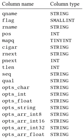
7.1 BAM record format. . . 57

7.2 Hive schema used for BAM data. . . 59

7.3 Data set size initially and after each modiﬁcation. . . 68

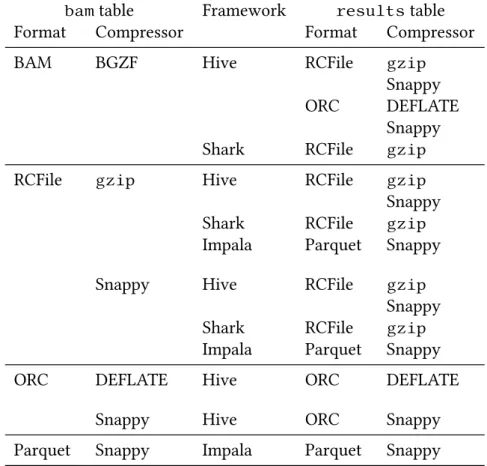
7.4 The experiment plan. . . 70

7.5 Unﬁnished 31-worker experiments. . . 72

8.1 The data set size in diﬀerent formats. . . 74

8.2 gzipvs. Snappy runtimes with Hive and RCFile. . . 90

8.3 BAM vs.gzip-compressed RCFile runtimes with Hive. . . 91

8.4 Hive runtimes withgzip-compressed RCFile vs. DEFLATE-compressed ORC. . . 92

8.5 RCFile vs. ORC runtimes with Hive and Snappy compression. 93 8.6 Impala vs. Shark runtimes on agzip-compressed RCFilebam table. . . 94

8.7 Runtimes of Impala with Snappy-compressed Parquet vs. Shark withgzip-compressed RCFile. . . 96

A.1 Hadoop settings given incore-site.xml. . . 104

A.2 HDFS settings given inhdfs-site.xml. . . 104

A.3 Hadoop MapReduce settings given inmapred-site.xml. . . 105

A.4 Relevant environment variables for Hadoop. . . 105

A.5 Hive conﬁguration variables. . . 106

A.6 Shark environment variables. . . 106

A.7 Parameters given inSPARK_JAVA_OPTS. . . 106

(14)

List of Figures

1.1 Historical trends in storage prices vs. DNA sequencing costs. . 3

2.1 Distributed MapReduce execution. . . 10

3.1 HBase state and operations. . . 25

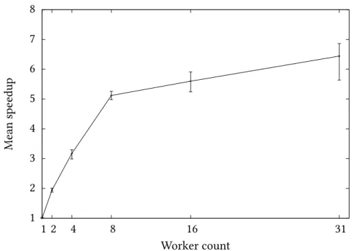
4.1 Speedup observed in BAM sorting with Hadoop-BAM. . . 30

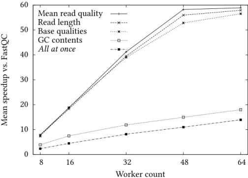
4.2 Speedup of SeqPig vs. FastQC. . . 31

8.1 Query times on a linear scale, by framework. . . 76

8.2 Query times on a log scale, by framework. . . 77

8.3 Impala’sbamquery times on a linear scale, by table format. . . 79

8.4 Hive’sbamquery times on a linear scale, by table format. . . . 80

8.5 Hive’sbamquery times on a log scale, by table format. . . 81

8.6 Hive’sresultsquery times on a linear scale, by table format. 82 8.7 Hive’sresultsquery times on a log scale, by table format. . 83

8.8 Hive’s post-BED join query times on a linear scale, by table format. . . 85

8.9 Shark’sbamquery times on a linear scale, by table format. . . 86

8.10 Shark’sbamquery times on a log scale, by table format. . . 87

8.11 Shark’s post-BED join query times on a linear scale. . . 88

(15)

List of Listings

7.1 HiveQL initializing RCFile withgzipfor Hive. . . 64

7.2 HiveQL used on thebamtable in Hive. . . 65

7.3 HiveQL used on theresultstable in Hive. . . 67

B.1 HiveQL code describing the table schema. . . 109

B.2 HiveQL used to createbamin BAM. . . 110

B.3 HiveQL used to createbamin RCFile. . . 110

B.4 HiveQL used to createbamin ORC. . . 110

B.5 HiveQL used to createbamin Parquet. . . 110

B.6 HiveQL used to create the BED table. . . 110

B.7 RCFile compression settings used with both compressors. . 110

B.8 The RCFilegzipcompression setting. . . 111

B.9 The RCFile Snappy compression setting. . . 111

B.10 HiveQL initializing post-BED join benchmarking in Shark. 111 B.11 HiveQL initializing single-node post-BED join benchmark-ing in Impala. . . 111

B.12 The parallelism setting for Hive and Shark. . . 111

B.13 Initial counting statements on the full data set. . . 111

B.14 Statements computing the two histograms. . . 112

B.15 Code specifying the columns in thebamtable. . . 112

B.16 The join with the BED table. . . 112

B.17 HiveQL copying the separately computed BED join data. . 113

B.18 HiveQL counting the size of the result of the BED join. . . 113

B.19 HiveQL computing the quality join and its size. . . 113

B.20 Simple ﬁlters and interspersed counts onresults. . . 114

(16)

(17)

C

1 Introduction

[A] wealth of information creates a poverty of attention, and a need to allocate that atten-tion eﬃciently among the overabundance of information sources that might consume it.

‘Designing Organizations for an Information-Rich World’ H A. S [Sim71] Data volumes nowadays are increasing to the point that many individual data sets are too large to be analysed, or even stored, on a single computer. Such data sets are known asBig Data, and can arise in several contexts. Examples include Internet searches, financial analytics, and various fields of science. Notably many Big Data problems can be found in the field of bioinformatics. A number of them are due to recent advances insequencing: the task of determining the base composition of e.g. DNA, possibly going as far as finding the entire genome of an organism.

In the case of DNA, the number ofbase pairsorbp, the building blocks of genomic information, that can be sequenced per unit cost has been growing at an exponential rate for over two decades, doubling approximately every 19 months [Ste10]. This alone would have caused Big Data issues sooner or later. However, the growth rate suddenly increased around the year 2005, due to the emergence of techniques known ashigh-throughput sequencing or HTS (a.k.a. next-generation sequencing or NGS). HTS has resulted in the process speeding up to the point that the cost has now been halving approximately every ﬁve months [Ste10]. As an example of current speeds, Pireddu, Leo, and Zanetti [Pir+11a] claim that their ‘medium-sized’ DNA sequencing laboratory can create 4–5 TB of data every week. At the high

(18)

1. I

end, BGI, ‘one of the largest producers of genomic data in the world’, generates 6 TB of data daily [Mar13]. For comparison, the largest hard disk drives available as of November 2013 are 6 TB in size [HGS13].

Exponential growth due to technological advances is not unusual in the computing world. Consider the following three ‘laws’:

• Moore’s law: the number of components in integrated circuits with minimum cost per component doubles every year [Moo65]. Later amended to a doubling every two years without the minimum cost as-pect [Moo75], and commonly quoted as 18 months [Int05]. Together with Dennard scaling [Den+07], Moore’s law has meant that pro-cessing power has doubled at essentially the same rate.1

• Butters’ law (of photonics): the cost of transmitting one bit over an optical network halves every nine months [Rey98].

• Kryder’s law, which was never given as a prediction, merely an obser-vation: areal storage density of hard disk drives had been increasing at a greater rate than the rate of processor improvement according to Moore’s law [Wal05].

Note, however, that none of the above growth rates, corresponding re-spectively to increases in processing power, network speed, and storage capacity, are even close to as fast as the pace at which sequencing is cur-rently improving. See Figure 1.1 for a clarifying plot comparing trends in storage and sequencing costs from 1990 to 2009. (For comparing the actual values instead of only the overall trends, one must know the size of a base pair, which depends on the storage format: for example, a single base is stored in 4 bits in BAM files and 8 bits in SAM files [SAM13], excluding compression.) Note that the source of the plot describes Kryder’s law as a doubling every 14 months, significantly more optimistic than more recent studies showing that the period is about 25 months [Kry+09]. Nevertheless, storing sequencing data on a hard disk is, or will soon be, actually more expensive than generating the data [Ste10], making its storage an increas-ingly difficult task. Discarding all but the most informative parts may be the only long-term option.

Small enough data sets may ﬁt completely in main memory, enabling computation that may be faster (per unit of size) than on larger sets by 1_{But the end of Dennard scaling made improving single-core CPUs much more}

diﬃcult than it was previously, leading manufacturers to turn to multi-core designs instead [Esm+11; Sut09]. Furthermore, there are signs that multi-core scaling will also not last long [Bos13; Esm+11; Har+11].

(19)

1990 1992 1994 1996 1998 2000 2003 2004 2006 2008 2010 2012 0 1 10 100 1,000 10,000 100,000 1,000,000 0.1 1 10 100 1000 10,000 100,000 1,000,000 10,000,000 100,000,000 Year

Disk storage (Mbytes/$)

DNA sequencing (bp/$)

Hard disk storage (MB/$) Doubling time 14 months

Pre-NGS (bp/$) Doubling time 19 months

-NGS (bp/$) Doubling time 5 months

Figure 1.1: Historical trends in storage prices vs. DNA sequencing costs. Reproduced from Stein [Ste10].

several orders of magnitude. Technological progress may result in this applying to current Big Data sets in as few as ten years: if current trends are followed, by that time the price of RAM (random access memory) will equal the current price of disk storage [Pla+11]. Thereafter many data sets that are currently considered Big Data may be able to be held fully in memory, with disk serving only as backup, in systems such as RAMCloud [Ous+11]. The speed at which e.g. sequencing data grows prevents such systems from being complete solutions to the problem of eﬃciently processing Big Data, but they can be very eﬀective for data sets that are not overly large.

Storage feasibility is only part of the picture: like any kind of raw data, sequencing data also needs to be analysed in order for it to be of any use. Clearly, if there is too much data for even its storage to be possible, its analysis is equally infeasible. This magnitude of data classiﬁes sequence data analysis as a Big Data problem.

For a problem to qualify as a Big Data problem, attempting to solve it with a single computer should result in one or both of the following:

• The computer has too slow a processor or too little memory to be able to perform the needed computations in a reasonable amount of time. Waiting for better hardware will not help, because the data growth outpaces Moore’s law.

(20)

1. I

• The computer does not have enough disk space to store the data sets on which computations are to be performed. Waiting for larger disk drives will not help, because the data growth outpaces Kryder’s law.

Therefore, in order to solve Big Data problems, lone computers are insuﬃ-cient. Distributed computing is required, i.e. having multiple networked computers, ornodes, working together in computer clusters. Ideally, the clusters used have been specialized for the task at hand, thus making them eﬀectivelywarehouse-scale computers[Bar+13].

Traditionally, distributed software has been created by developing com-munication protocols speciﬁc to the application, using primitives provided by e.g. MPI (the Message Passing Interface) [MPI93], the PVM frame-work [Sun90] or, in the data communications domain, the Erlang pro-gramming language [Arm97]. At this level, implementing the necessary functionality correctly is diﬃcult, especially if the software is to be run not only in small clusters but on warehouse-scale computers, with hundreds to tens of thousands of network nodes. Realizing high performance in such an environment is especially complicated. In addition, fault tolerance be-comes a necessity, because the probability of hardware failure is too high to ignore [Dea09].

To ensure that warehouse-scale distributed software can work at high performance and not worry about hardware failure, a framework speciﬁ-cally designed for that use case is necessary. One such framework was developed by Google [Goo]: MapReduce[Dea+04] coupled withGFS(the Google File System) [Ghe+03]. Together, they provide fault tolerance both for computations and data: most hardware failures neither interrupt run-ning processes nor cause data loss.

The implementations of the MapReduce system and GFS were not made publicly accessible, leading to the creation of Apache Hadoop [Had], an open source implementation of the same ideas. Hadoop has since expanded to become a collection of software related to scalable distributed computing.

Unfortunately, there exist problems for which MapReduce’s computa-tional model is far from ideal. In particular, MapReduce is specifically op-timized for throughput over latency, which makes it a poor fit forinteractive use. Interactive analysis tasks arise e.g. when users are not well enough ac-quainted with the data sets concerned to effectively perform long-running computations on them, having to insteadexplorethem with repeated que-ries, either narrowing down areas of interest or requesting more informa-tion according to newly realized needs [Hee+12]. MapReduce’s typical ten-second job startup time [Pav+09; Xin+12] guarantees that most users will shift their focus before a computation completes [Car+91], slowing

(21)

down this exploratory process. Interactive tasks are increasingly prevalent in sequencing data analysis [Che+12], making frameworks designed with latency in mind desirable. Low latency is a more diﬃcult goal to reach than high throughput [Dea+13; Pat04], but nevertheless such systems do exist. Two notable ones, whose performance is evaluated in this work, are Shark [Xin+12], which is based on Apache Spark [Zah+12], and Cloudera Im-pala [Imp], which is based on the design of Google’s Dremel [Mel+10]. Both frameworks allow access to structured data stored in HDFS (the Hadoop Distributed File System) using a language based on SQL (Structured Query Language) [Cha+74; Gro+09; ISO92], contributing to the trend [Mur+13] of handling interactive Big Data computations with ‘SQL-on-Hadoop’.

This Thesis proceeds as follows. In Chapter 2 the background of Map-Reduce as well as its specifics, especially pertaining to Hadoop, are gone over in detail. Next, Chapter 3 covers the Hadoop project and some notable high-level frameworks based on it: Apache Pig [Ols+08], the SQL-based Apache Hive [Thu+10a], and Apache HBase [HBa]. Chapter 4 surveys the current state of Hadoop in bioinformatics and presents two sets of tools developed by the author and his colleagues that enable using Ha-doop to manipulate and analyse sequencing data. Chapter 5 delves into the interactivity-oriented Shark and Impala frameworks. Chapter 6 discusses the importance of storage formats and studies the current state of the art formats in the worlds of sequencing and SQL-on-Hadoop. With the neces-sities covered, Chapter 7 presents a set of benchmarks used to compare the effectiveness of the exhibited SQL-based frameworks—Hive, Shark, and Impala—in interactive sequencing data analysis. The results obtained by running the benchmarks are examined in Chapter 8. Finally, Chapter 9 states some final thoughts based on the results of the experiments and the current state of scalable interactive sequencing data processing.

(22)

(23)

C

2 MapReduce

A computer’s attention span is as long as its power cord.

unknown Applying warehouse-scale computing to Big Data problems is not as simple as setting up the hardware. Programming for a warehouse-scale computer is a far more complex task than programming for a small cluster, which in itself is more challenging than programming for e.g. a typical desktop system. This is especially the case when performance is a concern, since eﬀectively utilizing all available resources involves co-ordinating several hardware and software layers. Examples of things to keep in mind are the complex memory hierarchy, heterogeneous hardware, failure-prone com-ponents, and network topology [Bar+13]: all in addition to the complexity of implementing the core of the application itself. As such it is no surprise that programming frameworks that ease the burden on the developer of warehouse-scale applications have been created. MapReduce [Dea+04] is one such framework, including automatic handling for data distribution and fault tolerance.

In order for a warehouse-scale computing framework to be practical, it must be able to tolerate hardware failure. Even with unrealistically reliable servers with a mean time between failures (MTBF) of 30 years, if there are 10 000 servers in a cluster, it will experience on average one failure every day [Bar+13]. This makes fault tolerance in software not only useful, but a practical necessity. In addition, it allows for a better price/performance tradeoﬀ by using relatively unreliable, cheaper hardware [Bar+03]. Map-Reduce has been designed with this in mind: it provides eﬃciently fault

(24)

2. MR

tolerant computations and is intended to be used together with ﬁle systems that provide fault tolerant data storage.

At its simplest level, MapReduce is a programming model for transform-ing data: the programmer need only specify two functions—theMap and Reduce functions—and the input data, and based on this information the corresponding output can be computed in a functional manner. Because of this, the model also allows for a simple strategy for fault tolerance: as executing a function with a given input will always result in the same out-put, e.g. all computations on a failed computer can trivially be re-executed on another computer, as long as the input data is still available. The Map-Reduce model allows for easy parallelization and is relatively simple to program for, making it an attractive choice for distributed computing.

However, the term ‘MapReduce’ in a distributed computing context is generally understood as meaning more than just the abstract programming model: it includes the associated implementation that handles scheduling the computation eﬃciently and dealing with machine failures during exe-cution.

The original MapReduce implementation [Dea+04] was developed in-ternally at Google and has not been released to the public. The currentde facto open source implementation of MapReduce is Apache Hadoop [Had], which will be discussed in Chapter 3. Hadoop’s existence makes Map-Reduce an attractive choice as a distributed computation model because Hadoop is well established, having seen use in a variety of ﬁelds with good results. (See Chapter 3 for detailed information.)

MapReduce is not perfect, though: its programming model can be considered too rigid for various tasks. For example, PACT [Ale+11] has been explicitly designed as an extension of MapReduce with the ability to express more complex operations. Another example, Spark [Zah+12], instead emphasizes data re-use: MapReduce does not intrinsically allow re-using intermediate results. If such re-use is desired, it must be done by manually saving and loading the corresponding data, which can incur needless I/O and serialization overheads. And of course, as previously mentioned (and elaborated on in Chapter 5), MapReduce is a very poor ﬁt for interactive work. In spite of these limitations, however, the MapReduce model continues to see use across a wide variety of applications.

In the following Sections the MapReduce execution model is discussed in detail before delving into the ﬁle systems that MapReduce is typically paired with. The information on MapReduce is based completely on Dean and Ghemawat [Dea+04] and White [Whi09].

(25)

2.1. Execution model

2.1 Execution model

Conceptually, the execution model of MapReduce consists only of applying theReduce function to the grouped results of theMapfunction. However, practical distributed MapReduce frameworks complicate the process: they specify more steps and implement them in certain ways to ensure that good performance and fault tolerance are achieved. Below, the simpler, conceptual model is ﬁrst brieﬂy explained, and then the principles that underlie the warehouse-scale implementations are considered.

The type signatures of the two user-speciﬁed functions form a concise description of the conceptual MapReduce execution model. See the fol-lowing, wherekis short for ‘key’ andv for ‘value’, the subscripts serve to diﬀerentiate the types, and the superscriptsm≥0,n >0, andp≥0denote

diﬀering list lengths:

Map ∶ (k1,v1) → (k2,v2)m

Reduce ∶ (k2,v2n) → v3p

As can be deduced from the type signatures, a MapReduce computation takes a sequence of key-value pairs as input, on which it performs the following tasks:

1. The Map function is applied to each key-value pair in the input, outputting any number of new key-value pairs for each one.

2. Each key in the output from the previous step is paired with all the values that were associated with that key.

3. TheReduce function is applied to each pair in the result of the pairing in the previous step. The resulting list of data forms the ﬁnal output. To clarify the process, consider the following simple example, where the task consists of taking as input a set of documents and outputting, for each word encountered, the set of documents it was found in. Here the input type could be e.g.(k1,v1) = (document-name,contents)for each document. TheMap function would go through the contents, outputting pairs of type(k2,v2) = (word,document-name). Thus the Reduce func-tion receives as input pairs of the form(word,document-namen), which

is precisely what was desired in the problem statement. The ﬁnal outputv3p would depend on the exact format in which the output is desired, but could be e.g. a string (just one string, i.e.p=1) of the form "word","document-1-name","document-2-name",…for each word.

(26)

2. MR

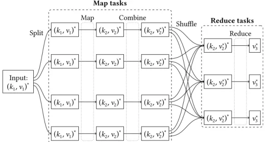
While the above description is suﬃcient for implementing a basic Map-Reduce framework, fully distributed systems for warehouse-scale com-puters, such as Google’s MapReduce implementation and Hadoop Map-Reduce, are more complex and perform the steps in a very speciﬁc way. See Figure 2.1 for a graphical overview of how MapReduce computations are executed on such systems.

(k1,v1)∗ (k2,v2)∗ (k2,v2∗)∗ (k2,v2∗)∗ v3∗ (k1,v1)∗ (k2,v2)∗ (k2,v2∗)∗ Input: (k1,v1)∗ (k2,v ∗ 2)∗ v3∗ (k1,v1)∗ (k2,v2)∗ (k2,v2∗)∗ (k2,v2∗)∗ v3∗ (k1,v1)∗ (k2,v2)∗ (k2,v2∗)∗ Split Shuﬄe Map Combine Reduce Map tasks Reduce tasks

Figure 2.1: Distributed MapReduce execution with four map tasks and three reduce tasks. k_i andv_j denote key typeiand value type

jrespectively. The asterisk superscripts denote unknown list lengths.

Distributed MapReduce is structured as a master-slave system. The master node (known in Hadoop as thejobtrackerand predefined as a specific node for the whole cluster) allocates workers for different parts of the computation and co-ordinates communication between them. The slaves (known in Hadoop astasktrackers) are the nodes that actually read the input data, run theMapandReduce functions, and write the output data. Each slave node provides a number of map and reduceslotsfor running the two different functions. For a computation orjob, typically the user selects the number of reduce tasks to be performed while the MapReduce system automatically determines the number of map tasks. The full execution process is as follows:

1.Split This step is performed solely on the master. The input ﬁles are conceptually split into chunks: a set ofsplits, i.e. tuples that identify

(27)

2.1. Execution model

sequential parts in the input ﬁles, is created. These splits are typically tens of megabytes in size, often corresponding to the block size of the ﬁle system in use (see Section 2.2). Based on this the master creates a map task for each split and assigns as many of them as it can to separate map slots, which are started up and begin running. (The remaining tasks are started as the job progresses: when a task completes it frees its slot for use by another task.)

2.Map Each map task involves reading the corresponding input split, forming key-value pairs of the data therein, and handing them to the Map function for processing. These intermediate key-value pairs are written to local disk, sorted by key, andpartitioned: diﬀerentiated based on which reduce task they belong to. The default partitioning simply assigns each keyk to the reducerh(k)modR whereh is a

hash function [Knu73] andR is the number of reduce tasks.

3.Combine This is an optional step that essentially runs theReduce func-tion on the partifunc-tioned output of theMapfunction directly as part of the map task. While a customCombinefunction can be given, typic-allyReduce is used as-is. This use requires that it be commutative and associative. Note that since combining can reduce the map task’s out-put size, it is performed before writing the partitions to local disk, as long as the task has enough available memory for in-memory sorting and partitioning. This way, fewer I/O operations are performed. 4.Shuﬀle The map tasks communicate the locations of their partitioned

outputs to the master node. It then notiﬁes the corresponding reduce tasks (starting them up in reduce slots as required) that new data is available. The reduce tasks read the data from the local disks of the nodes where the data was written—note that this may be the same node on which the reduce task itself is running, in which case no network communication is required. When a reduce task has received all of its input data, it sorts it so that it is grouped by key.

5.Reduce Each reduce task iterates over its sorted sequence of key-value pairs, passing each unique key and corresponding sequence of values to theReduce function. The output from it is written directly to the output file of the reduce task, which is one of the final output files generated by the MapReduce computation.

The end result is a set of output ﬁles, one from each reduce task. They are not automatically combined to a single ﬁle because that is not always

(28)

2. MR

necessary: they could be used as-is as inputs for another MapReduce job, for example. It is also possible to run amap-only jobin which only theMap function is used, with the map tasks’ output forming the output for the entire computation.

Fault tolerance in this kind of a fully distributed MapReduce system is fairly simple to implement. The master node periodically pings the slaves, assuming them to have failed if it does not receive a response in time. In-progress tasks on failed nodes are rescheduled and eventually restarted. Completed map tasks are also rescheduled, but completed reduce tasks are not. This is because the input and output ﬁles are assumed to be on a shared storage system, separate from the local disks that are used for storing the intermediate output from map tasks. Thus, if a node with a completed map task whose output has not yet been sent to a reduce task fails, the map task needs to be restarted, but if a node with a completed reduce task fails, nothing needs to be done. This way worker failure is fully accounted for, which is important for long-running jobs at warehouse scale. In contrast, master failure is deemed unlikely since it requires a speciﬁc node to fail, and is not handled at all, making the master a single point of failure.

Sometimes worker nodes may have unexpectedly poor performance due to e.g. faulty hardware. This results instragglers: members of the last few map or reduce tasks which take a particularly long time to complete, holding up the whole computation. A key optimization in MapReduce systems, that of speculative or backup execution, was designed to mitigate this problem. After all tasks have been started, if some tasks have been running for a relatively long time and seem to be progressing (performing I/O of key-value pairs) relatively slowly, the master attempts to reschedule those same tasks on different nodes. When a task is successfully completed, any other executing duplicates of that task are stopped. Speculative execution does not significantly affect the resources used by a job but can speed it up greatly.

Since tasks can run multiple times as well as be restarted at any point, the Map andReduce(andCombine, if used and distinct fromReduce) functions should be free of side eﬀects: pure functions of their input values. Only then is it guaranteed that all the output of a fully distributed MapReduce system is equivalent to a single sequential execution of the program. In the face of nondeterministic user-supplied functions, the output of each reduce task may correspond to a diﬀerent sequential execution. Whether this inconsistency is a problem in practice depends on the application.

(29)

2.2. Distributed ﬁle system

2.2 Distributed ﬁle system

MapReduce is traditionally paired with a specific distributed file system, designed for large files and streaming access patterns. For Google’s Map-Reduce that file system is GFS (the Google File System) and for Hadoop it is HDFS (the Hadoop Distributed File System). Both share similar design principles and implementation strategies, which will be covered in the remainder of this Section. Information on GFS in this Section is based on Ghemawat, Gobioff, and Leung [Ghe+03] and information on HDFS is based on White [Whi09], except where otherwise indicated.

GFS and HDFS are both, like MapReduce, master-slave systems. The master node (known in Hadoop as thenamenode) keeps track of the state of the slaves as well as ﬁle metadata, and the slave nodes (known in Hadoop as thedatanodes) are responsible for all data storage and communication. Replication is used to provide fault tolerance: each block is stored on multiple slaves—three by default. For simplicity reasons [McK+09] the master node is a single point of failure, though HDFS’ssecondary namenode can limit data loss in case of catastrophic master node failure.

When using MapReduce, the slave nodes should be used to run Map-Reduce workers as well, allowing MapMap-Reduce to take advantage of data locality for map tasks. This is done by scheduling map tasks on nodes where the data for that task’s split is stored, or, failing that, on nodes that are nearby in terms of the network topology. Replication is advantageous here as well as for fault tolerance, since it improves the odds of being able to schedule a task on a node that has the corresponding split’s data available locally. Note that it is possible to run a MapReduce job on GFS and HDFS without any of the input data being sent across the network.

A major design principle of both GFS and HDFS is to support large files efficiently. ‘Large’ in this context means at least 100 megabytes, but typically several gigabytes, and up to terabytes. In contrast, small files are assumed to be rare, and so are not optimized for at all. This is very much the opposite of what file systems are traditionally optimized for [Gia99], which is one of the main reasons that GFS and HDFS are typically paired with MapReduce; they are both intended for Big Data sets consisting of large files.

Another important design principle of GFS and HDFS is the emphasis onwrite-once, read-manyoperation and streaming reads: written files are assumed to be modified rarely if at all, and workloads are expected to in-clude reading entire files or at least significant portions of them. Random reads and writes are not optimized for—in fact, HDFS does not support ran-dom writes at all. This lack of arbitrary modifications makes implementing

(30)

2. MR

replication much simpler, and the philosophy of large reads makes band-width far more important than latency. Once again, this ties in with the way MapReduce works, but it is also a more generally helpful restriction for scalable storage architectures: for example, the lowest layer of the Win-dows Azure Storage [Cal+11; WAz] system has the same limitation.

A notable result of these design decisions is that the block size of both GFS and HDFS is unusually large: 64 MiB. (HDFS does allow changing this, but reducing it to usual file system block sizes would be self-defeating.) This reduces overhead related to metadata management, mainly by drastically reducing the amount of metadata: compared to a more traditional 4 KiB block size and assuming a large enough file, 16 384 times less blocks have to be kept track of. Thus metadata can be kept fully in the memory of the master, making metadata operations fast and enabling easy rebalancing (replica distribution) and garbage collection. Keeping metadata in memory has a drawback, however: it makes the capabilities of the master limit the number of files that can be stored [McK+09]. Another benefit of large block sizes is that if the time to read a full block is much greater than the physical seek time of the disk drives used, reading a file consisting of multiple arbitrarily distributed blocks operates at a speed close to the drives’ sequential read rate.

(31)

C

3 Apache Hadoop

First, solve the problem. Then, write the code. unknown Apache Hadoop [Had; Whi09] was originally conceived as a nameless part of the Nutch [Nut] Web search engine, implementing open source versions of MapReduce [Dea+04] and GFS (the Google File System) [Ghe+03] for its own purposes, in the Java programming language [Gos+13]. Yahoo! [Ya!] soon began contributing to the project, at which point these components were separated, forming the Hadoop project, named after the creator Doug Cutting’s child’s toy elephant. At around the same time, Hadoop began to be hosted by the Apache Software Foundation [Apa], giving it the full name ‘Apache Hadoop’. Since then, Hadoop has grown to become a collection of related projects, two of which are the original MapReduce and ﬁle system components: Hadoop MapReduce and HDFS (the Hadoop Distributed File System).

For most of Hadoop’s history, the MapReduce component has been the only computational framework supported in Hadoop. Tasks running on other systems, e.g. MPI [MPI93], have not been able to be scheduled on Hadoop clusters. This has meant that the machines in a cluster should be conﬁgured to run only one class of tasks, such as Hadoop MapReduce jobs or MPI processes. Otherwise, one node may have several computationally intensive tasks running at once, possibly resulting in resource starvation issues such as running low on memory or disk space, which may in turn cause all tasks on the node to fail. On the other hand, the traditional solu-tion of partisolu-tioning the cluster by framework can lead to poor resource utili-zation, with some machines remaining completely idle while there is work

(32)

3. A H

to do, just because they have been configured for a different framework. Apache Mesos [Hin+11; Mes] is a cluster manager with cross-framework scheduling, solving this problem more effectively. The latest releases of Hadoop (the 2.x series) include their own similar system, calledYARN (Yet Another Resource Negotiator [Wat12]) [Mur12; YRN; YRN13], also known as NextGen MapReduce or MapReduce 2.0. In addition to cross-framework scheduling, YARN also removes the concept of map and reduce slots from MapReduce slave nodes, instead dynamically allocating map and reduce tasks according to what is most needed at the time. YARN takes over some of the cluster management responsibilities currently handled by Hadoop MapReduce, allowing other computational frameworks to effectively co-exist within Hadoop.

Several companies provide their own distributions of Hadoop, for which they also naturally oﬀer commercial support. The most notable such com-panies are Cloudera [Clo], Hortonworks [Hor], and MapR [MaR]. They are naturally all major contributors to Hadoop, but have their own exten-sions as well. Hortonworks’s distribution is the only one with support for running on Windows Server. Their contributions are also particularly note-worthy for theirStinger Initiative[StI], which involves improving the per-formance of the Hive project, which is presented in Section 3.2. Cloudera Impala [Imp] is a distributed query engine meant for interactive use, as opposed to MapReduce’s emphasis on throughput, and is further discussed in Chapter 5. MapR’s distribution provides fault tolerance for the master in both MapReduce and HDFS: the jobtracker is restarted on failure and the namenode is fully distributed. MapR is also unique in that it does not use HDFS; a complete rewrite in the C++ programming language [Str13], whose interface is nevertheless compatible with HDFS, is used instead.

Usage of Hadoop within an organization is unlikely to encompass the entire range of Hadoop-related projects. Some may not even use the Map-Reduce component, due to the existence of other computational engines and YARN. One thing, however, is common to almost all users of any part of Hadoop: HDFS. The amount of data an organization has stored in HDFS is an indication both of how much the organization uses Hadoop and of what kinds of data volumes Hadoop has been used for. For demonstration purposes, the following is a sample of HDFS usage:

• As of 2013, Facebook [Fac] stores more than 300 PB of data ‘in a few large Hadoop/HDFS-based clusters’ [Pre; Tra13]. In 2010, they stored 15 PB of data with 60 TB being added daily, and with compression reducing the space usage to 2.5 PB and 10 TB respectively [Thu+10b]. Clearly the rate at which data is added has increased since then, or

(33)

3.1. Apache Pig

they would not have reached the 300 PB mark yet.

• In 2010, Yahoo! had over 82 PB of data among over 25 000 servers split into clusters of about 4000 [Ree10].

• In 2010, Twitter [Twi] had ‘(soon) PBs of data’, with 7 TB of new data coming in every day [Wei10].

Chapter 2 already detailed MapReduce and HDFS. In the following Sec-tions, three prominent open source projects related to Hadoop are instead discussed. Each oﬀers its own higher-level abstraction on top of Hadoop MapReduce and HDFS. Apache Pig oﬀers a high-level language for express-ing MapReduce programs, Apache Hive provides a data management and querying system using an SQL-like language implemented with MapReduce, and Apache HBase allows scalable random access into a key-value store in HDFS.

3.1 Apache Pig

Apache Pig [Ols+08; Pig], originally developed by Yahoo!, is a high-level interface to MapReduce, providing a custom query language for bulk data manipulation called Pig Latin. Pig Latin is compiled into a sequence of MapReduce computations which are executed on Hadoop. Pig drastically lowers the bar of using Hadoop MapReduce, giving users a richer pool of primitives they can use to describe their computations and not requiring them to implement it in Java, a far more low-level programming language than Pig Latin. This can greatly simplify development and maintenance, improving programmer productivity. Similarly, Pig can be used as a high-level way of implementing what is known as an ETL (Extract, Transform, and Load) pipeline [Sha+12].

Pig treats all data as relations. Relations are defined as bags (a.k.a. multisets) of tuples. The fields in the tuples can be simple values like integers or strings, but also complex like key-value mappings or even other bags and tuples—arbitrary nesting is allowed. Tuples in a relation are not constrained in any way: they can have different numbers of fields as well as different field types in the same position. It is possible, however, to define a schemawhich specifies a common type for the tuples in a relation. Without a schema, Pig infers a ‘safe’ type for every field (such as double-width floating point for all numbers), which can cause performance to suffer.

The data model is similar to that used by traditional relational data-base systems [Cod70] but more ﬂexible. The lack of a deﬁned ordering is

(34)

3. A H

particularly useful for MapReduce processing, as it does not restrict the par-titioning strategy (how map outputs are spread among the reducers) in any way. In addition, allowing arbitrary nesting can simplify operations com-pared to only having ﬂat tables, especially if they are normalized [Dat06], since all data can be kept in one relation instead of having to perform join operations when needed.

Pig Latin has severalcommandsfor working with relations, and more are being added as development proceeds. The following list is incomplete but representative:

• LOADandSTOREinteract with external storage, respectively reading and writing relations.

• Standard embarrassingly parallel commands: FOREACHtransforms

every tuple in a relation andFILTERselects tuples from a relation based on a condition.

• Commands related to ordering and equality: ORDER BYperforms sorting, RANK adds ﬁelds describing sort order but preserves the existing order, andDISTINCTremoves duplicates.

• Grouping: GROUPa.k.a.COGROUP, which can be applied to more than one relation at a time.

• Joins:CROSSandJOINcan be used to respectively form the Cartesian product or any kind of inner or outer join [Gro+09; ISO92] of two or more relations.

Most commands can utilize functions to specify their exact eﬀects. For example,FOREACHcould be used asFOREACH r GENERATE f(x)where

ris a relation,fa function, andxa ﬁeld contained in the tuples ofr. The result of the command is a relation containing 1-tuples whose values are given by the functionfon the ﬁeldxof each tuple inr. There are many built-in functions, including arithmetic operators as well as aggregating functions such asCOUNT, which computes the number of tuples in the given relation.

Clearly, these operations by themselves are much more expressive than the MapReduce model, but Pig Latin can also be extended by users. While the command set cannot be changed without modifying Pig itself, new functions can easily be added. Furthermore, the ﬂexibility of the data model means that all user-deﬁned functions can be used in any function-using command without restriction, unlike e.g. in Hive whereSELECTclauses only allow using scalar functions.

(35)

3.2. Apache Hive

Pig has been widely adopted. In June 2009 at Yahoo!, 60% ofad hoc and 40% of production Hadoop MapReduce jobs came through Pig, and further increases in Pig usage were expected [Gat+09]. A cross-industry study performed in 2012 showed three out of seven analysed clusters hav-ing signiﬁcant Pig usage, one of which was observed to have had over 50% of MapReduce jobs submitted via Pig [Che+12]. LinkedIn [LiI] uses Pig both for user-facing data set generation and for analytics [Aur+12]. The reported runtime increase when using Pig instead of hand-written Map-Reduce has ranged from a factor of 1.3 [Sha+12] to 1.5, but it has improved signiﬁcantly over time and is likely to continue to do so [Gat+09]. This level of performance loss seems to be acceptable in practice: consider that Twitter was using ‘almost exclusively’ Pig for its analytics in 2011 [Lin+11].

3.2 Apache Hive

Apache Hive [Hiv; Thu+09; Thu+10a] is a data warehouse system built on top of Hadoop: essentially, it is a high-level interface to both MapReduce and the backend storage system, which is typically HDFS, but can also be HBase (see Section 3.3). Hive enforces a structural view, very similar to traditional relational database systems [Cod70], of the data sets it handles. They are queried and manipulated using a language based on SQL (Struc-tured Query Language) [Cha+74; Gro+09; ISO92] calledHiveQL, which is translated to MapReduce computations. Hive was originally developed by Facebook; later, Google created a very similar warehousing solution called Tenzing [Cha+11]—a rare example of outside ideas being incorporated so directly at Google, instead of the other way around.

Hive’s data model is based ontables, akin to those used in relational databases. Records of data are stored inrows, which are split among a set of typedcolumns, which are in turn deﬁned in aschema. A row may have a null value in any column, but each row in a table always has the same amount of columns. Possible column types include primitive types such as integers and strings as well as complex types: arrays, key-value mappings, and product and sum types calledstructsandunions.

All metadata about the tables managed by Hive is catalogued in the metastore. The existence of the metastore, i.e. keeping track of persistent metadata about data sets, is what makes Hive a data warehouse system as opposed to purely computational systems such as Pig. The metastore re-members all tables and all information about them; primarily their schemata. Because it is randomly accessed, the metastore is not stored in HDFS. In-stead, a traditional relational database is used.

(36)

3. A H

Various settings for performance tuning may be applied to tables in Hive. Tables can bepartitioned on certain columns, so that rows with the same combination of the partitioned columns’ values are stored together. Partitions may furthermore bebucketed, which is another layer of partition-ing based on the hash of a spartition-ingle column. Table rows can also be stored in sorted order. When using HDFS storage, tables map directly to directories, partitions to subdirectories of their table’s directory, and buckets to ﬁles in their partitions’ directories.

Notably, even though Hive manages storage of tables, it does not rely on any particular file format. As long as the contents of each file can be serialized for storage and deserialized (using a Java class called aSerDe) for manipulation in HiveQL according to the table’s schema, the files com-prising the data of one table can even be in completely different storage formats.

Hive supportsindexing on table columns, a classical strategy for speed-ing up query operations in databases. The trade-off is that the index takes up some additional storage space and modifications become slower as the index needs to be updated. Considering that Hive’s main use case, data warehousing, consists of managing very large and mostly immutable data sets, the slowdown is irrelevant and the amount of space taken by the index is likely to be negligible, whereas the query speedup is likely to be very welcome. Hive currently provides two kinds of indices: one that identifies HDFS blocks for the rows corresponding to a given key, and a bitmap in-dex [Cha+98] that also identifies which rows in the blocks are populated with that key.

HiveQL currently (as of version 0.12) has two kinds of data manipulation statements:LOAD, which simply copies data ﬁles into the appropriate HDFS directory of the table, andINSERT, which writes the results of aSELECT

clause into a table while performing appropriate format conversions. LOAD

is an optimization, relying on the user to make sure that the ﬁle is usable in the table as-is, lest the table end up in an unusable state. INSERTis

more flexible, as it can insert into more than one table at once and compute the partitioning dynamically. There are no other manipulation statements: HiveQL currently has no way of updating or deleting rows. This makes sense, given that rows are typically contained as-is in files in HDFS, which does not support in-place modification of files.

Querying in HiveQL is done with theSELECTstatement, like in SQL. Various clauses to modify the statement’s behaviour are supported, as in any modern SQL system. The following is a sample of what is available:

(37)

3.2. Apache Hive

• DISTINCTremoves duplicates from the result. • GROUP BYgroups data by the given columns’ values.

• Sorting clauses: ORDER BYandSORT BY, the latter of which only guarantees sorting the output of each reduce task, thereby forming a partially ordered result. ORDER BYperforms a global sort, but one must use the new Hive 0.12, or a later version, to avoid a poor implementation in which all data is sent to a single reduce task for sorting [HIV10].

• Combining the results of many selections in one query withUNION ALL.

• Joins: the various forms of JOINcan compute any form of inner or outer join [Gro+09; ISO92] of two or more tables, as well as the Cartesian product.

All in all the functionality available is very similar to that offered by Pig Latin, though HiveQL is not quite as flexible due to Hive’s stricter data model. Nevertheless, just like Pig Latin, HiveQL can also be extended by users via user-defined functions. Hive users can define three kinds of functions: ordinary ones, which simply transform one row into another and are therefore always run within map tasks;table-generating functions, which can transform one row into multiple rows; andaggregation functions, which can combine multiple rows together and thus are run in reduce tasks, or in map tasks as part of aCombinefunction.

Hive also has support for creating views based on SELECT queries. Views are essentially named queries that are saved in the metastore, which can themselves be queried just like tables can. Conceptually, when a view is queried, the result of the view’s deﬁning query is computed, and then the original query is evaluated on that result. In practice, the two queries may ﬁrst be combined into a single one which is executed directly on the tables used.

Hive has seen wide adoption. As the originator of Hive, Facebook has naturally been a heavy user, with over 20 000 tables and several petabytes of data in a Hive cluster in 2010 [Thu+10b]. As of 2013, their data ware-house, which likely continues to be largely Hive-based, has grown to over 300 PB [Pre; Tra13]. LinkedIn uses primarily Hive and Pig for its internal analytics [Aur+12]. A cross-industry study performed in 2012 showed four out of seven analysed Hadoop clusters having signiﬁcant Hive usage, three of which had 50% of their MapReduce jobs, sampled over time periods ran-ging from days to months, submitted via Hive [Che+12].

(38)

3. A H

As Hive is used especially for analytics, the fact that it makes use of the purely throughput-optimized MapReduce as a computational backend has been considered problematic. In an interactive setting the startup costs of a Hadoop MapReduce job are not necessarily insigniﬁcant, as they can even dominate the execution time of short computations [Pav+09]. Frameworks that attempt to solve this problem are presented in Chapter 5.

3.3 Apache HBase

Apache HBase [HBa] is an open source distributed data storage system based on the design of Google’s Bigtable [Cha+06], enabling random read-write access to individual records in Big Data sets. This is a key advantage over HDFS or MapReduce, which only provide streaming access. In addi-tion, as bulk operations on HBase tables can be performed using Hadoop MapReduce, no functionality is lost by relying on HBase instead of HDFS for data storage—though performance is of course lower than when using HDFS directly. HBase was originally conceived by Powerset as a founda-tion for their natural language search engine [Geo11]; though the engine never materialized (because Powerset was acquired by Microsoft before the engine was completed), HBase continues to be developed under the Apache Software Foundation.

HBase provides sorted three-dimensional lookup tables in a manner similar to traditional relational database engines, but with a much simpler data model, namely:

(row ∶ string,column ∶string,version∶ int64) →string

In other words, each data value, orcell, in a table is uniquely identified by arow,column, andversion, of which the rows, columns, and values are simply arbitrary byte strings while versions are 64-bit integers—typically timestamps. Data is sorted first by row, then by column, and finally by version, with later versions coming first in the sort order. This simple model allows scaling by just adding more nodes, without having to worry about maintaining the complex invariants to which relational databases adhere [HBR; Whi09].

HBase has a very simple interface to tables, consisting of only four operations (excluding metadata-related functionality):

1. Get: reads a row, possibly limiting the result set further to speciﬁc columns and/or versions.

(39)

3.3. Apache HBase

2. Put: writes a row, either adding a new one or replacing an existing one.

3. Delete: removes a row.

4. Scan: iterates over a sequential range of rows, returning one at a time to the user.

This limited set of functionality makes HBase’s essential nature as a key-value store evident: HBase itself does not provide the more complicated operations that are typically found in database systems, such as joins. As previously mentioned, however, Hive can use HBase as a storage backend, allowing that kind of functionality to be used on data stored in HBase.

As MapReduce handles scheduling computations on a distributed sys-tem, so does HBase take care of distributing the data it stores among the available nodes. Tables in HBase are automatically partitioned into se-quences of rows calledregions, which can be distributed among the HBase servers, aptly calledregionservers. This spreads out computational load on the table as well as the data itself, enabling large tables to utilize the entire cluster’s storage space.

HBase naturally also includes fault tolerance, which is mostly reliant on a reliable storage system, typically provided by HDFS. As with MapReduce and HDFS, it is based on a master-slave architecture where the master only co-ordinates the slaves and monitors their health. The slaves in an HBase cluster are the aforementioned regionservers. Unlike MapReduce and HDFS, HBase provides fault tolerance for the master node: this is facilitated by using Apache ZooKeeper [Zoo], a co-ordination service based on the Zab algorithm [Jun+11] (similar but not identical to the classical Paxos algorithm [Lam98]). ZooKeeper is used to make sure that only one master is active at any given time, and also to store various metadata about the cluster.

Fault tolerance on the regionservers requires some work due to the method used to implement write operations. For performance, writes (including additions, modifications, and deletions) are performed on in-memory caches calledMemStores(in Bigtable,memtables) and only flushed periodically, to HDFS files calledStoreFiles orHFiles(corresponding to the BigtableSSTables, short for Sorted String Tables [McK+09]). Data loss is prevented by also logging writes to HDFS: when a regionserver fails, its log is replayed by all replacement regionservers (i.e. all servers that are assigned any region that was previously assigned to the failed server), bringing them up to date. Note, however, that currently (as of version 0.96) HBase does not ensure that log entries are flushed to physical disks before proceeding

(40)

3. A H

with the operation [HBA12; Hof13]: therefore, in the event of power loss or a similar catastrophic failure, data loss can still occur.

Recall that HDFS does not allow modifying files. Thus, whenever a regionserver decides to flush a MemStore to HDFS, it creates a new StoreFile for the contents of the cache. Read operations must, in the worst case, consult the MemStore as well as all StoreFiles. As data is kept in sorted order, e.g. reads requesting only the latest version of a record might need to consult only the MemStore, but in the worst case, a read operation involves traversing the whole MemStore as well as all StoreFiles before the appropriate values to return are found. To prevent having to consult too many StoreFiles, they are periodically merged into a single StoreFile in a process calledmajor compaction. At this point, all deletions are also fully handled: when a cell that is not currently in the MemStore is deleted, the delete operation is merely noted in a marker called atombstone and eventually flushed, but the supposedly deleted cell still persists in the older StoreFiles. The cell and the corresponding tombstone are actually removed from storage only during a major compaction, when they are discarded from the final, merged StoreFile. Minor compactions, in which only a subset of the StoreFiles are merged and deletions are not processed, also occur occasionally.

Figure 3.1 provides a graphical overview of how operations in HBase aﬀect the diﬀerent kinds of state. In summary:

1. Write operations, including additions, modiﬁcations, and deletions, are logged and then applied to the MemStore.

2. The MemStore is eventually ﬂushed, creating a new StoreFile. 3. StoreFiles are eventually merged together into a single StoreFile

during a minor or major compaction.

4. Read operations access all StoreFiles and the MemStore.

Since StoreFiles are written only when flushing or compacting, the amount of records written at a time is typically quite large. Therefore compression can be utilized more effectively than in systems that simply modify or append to existing files: each StoreFile can be compressed as a whole at its creation time, resulting in a better compression ratio than could otherwise be achieved. Additionally, as major compactions are usually run when the HBase cluster is not under heavy load, it is possible to apply a relatively resource-intensive but effective compression algorithm on a large amount of data at once, improving compression ratios even further. (For some information about compression, see Chapter 6.)

(41)

3.3. Apache HBase

HDFS Memory

MemStore

New

StoreFile StoreFile StoreFile

Log Write Flush Read Merge New merged StoreFile

Figure 3.1: HBase state and operations. ‘Read’ includes both single-row reads and scans and ‘Write’ includes single-row additions or modiﬁcations as well as deletions. The boundary between HDFS and the MemStore is shown as a dotted line.

Having to read from several HDFS files for every read operation would be prohibitively slow. Hence, to speed up reads, regionservers cache parts of StoreFiles as well as individual lookup results, and allow using Bloom filters [Blo70] to quickly exclude StoreFiles from being considered for a query. Bigtable tests in Chang et al. [Cha+06] show that despite these efforts, random access reads were approximately an order of magnitude slower than similarly random writes, and sequential reads were either significantly slower or faster than sequential writes. Results from the Yahoo! Cloud Serving Benchmark [Coo+10] in 2010 demonstrated similar behaviour in HBase: while it dominated the competition in write-heavy workloads, HBase was comparatively slow in performing read operations.

Facebook has used HBase heavily with positive results: in 2011, Face-book’s HBase clusters consisted of thousands of nodes implementing diﬀer-ent kinds of applications, including real-time messaging among millions of users [Aiy+12; Bor+11]. Several other industrial users of HBase exist [HBP],

(42)

3. A H

but none have (or have published information about) notably large cluster sizes or data volumes.

(43)

C

4

Hadoop in bioinformatics

In 26 years of software engineering, I have never come [across] a problem domain that I found stable enough to trust.

R C. M [Mar96] The ﬁeld of bioinformatics contains a large number of Big Data problems, especially in sequencing data analysis. The tools oﬀered in the Hadoop project have been heavily used in implementing various solutions, although other systems—mainly the Message Passing Interface, MPI [MPI93]—have been the method of choice for some projects [Tay10].

A task that has seen a significant amount of attention issequence align-ment or mapping: similarity search between two or more sequences in order to estimate either the function or genomic location of the query se-quence. Alignment is an important part of almost any analysis process. As such, it is not surprising that much effort has been spent in developing efficient and scalable alignment methods.

CloudBurst [Sch09] and CloudAligner [Ngu+11] are examples of se-quence aligners based on Hadoop MapReduce. CloudAligner is notable in that it uses map-only jobs to achieve greater performance. The publica-tion that presented the Hadoop-based CloudBLAST [Mat+08] compared it against a similar MPI implementation, mpiBlast [Dar+03], ﬁnding that CloudBLAST performed up to approximately 30% better and was simpler to develop and maintain. Many MPI-based aligners [dAra+11; Mon+13; Rez+06] have nevertheless been created.

Alignment tools often include other features, either as additional utilities or because they are intended for some speciﬁc analysis for which alignment

(44)

4. H  

is only a part of the process. The following are all examples that use Hadoop MapReduce for scalability. Seal [Pir+11a; Pir+11b] provides an aligner which includes postprocessing, such as duplicate read removal. Crossbow [Lan+09], Myrna [Lan+10], and SeqInCloud [Moh+13] implement sequence alignment as part of their speciﬁc analysis pipelines.

Sequence alignment is, of course, not the only analysis task in bio-informatics for which Hadoop has been utilized. The SeqWare Query Engine [OCo+10] uses HBase to implement a database for storing sequence data. MR-Tandem [Pra+12] carries out protein identiﬁcation in sequence data using MapReduce. CloudBrush [Cha+12] and Contrail [Sch+] use MapReduce in performing a process called de novo assembly: assembly of previously unknown genomes from sequence data. SAMQA [Rob+11] detects metadata errors in sequence data ﬁles, using MapReduce for paral-lelization.

Finally, some projects provide support facilities, making it easier for their users to implement the complete analysis pipelines. The Genome Analysis Toolkit (GATK) [McK+10] is one example. It is based on the MapReduce model but does not use Hadoop, instead running on a custom engine and having a separate wrapper for distributed computing called GATK-Queue [GAQ]. The aforementioned Seal project, while focused on alignment, presents its functionality as a set of tools that can be used for other purposes as well. Cloudgene [Sch+12] is a platform providing a graphical user interface for executing bioinformatics applications based on Hadoop MapReduce, with support for several of the tools mentioned here. BioPig [Nor+13] is a Pig-based framework containing various useful functions, including wrappers for some other commonly used applications.

The author and his colleagues have developed two supporting tool sets of their own, oﬀering useful functionality that was not previously available. Hadoop-BAM is a library providing ﬁle format support along with some useful command-line tools, and SeqPig is a higher-level interface in Pig including special functionality for sequence data analysis. They are presented in the following two Sections.

4.1 Hadoop-BAM

Hadoop-BAM [HBM; Nie+12; Nie11] is a library written in the Java pro-gramming language, providing support for using Hadoop MapReduce to manipulate sequencing data in various common ﬁle formats. Currently, as of version 6.0, the formats supported are all of the following: