Separators and Treewidth
Thomas Bläsius
1, Tobias Friedrich
2, and Anton Krohmer
3 1 Hasso Plattner Institute, Potsdam, Germany2 Hasso Plattner Institute, Potsdam, Germany
3 Hasso Plattner Institute, Potsdam, Germany
Abstract
Hyperbolic random graphs share many common properties with complex real-world networks; e.g., small diameter and average distance, large clustering coefficient, and a power-law degree sequence with adjustable exponentβ. Thus, when analyzing algorithms for large networks, potentially more realistic results can be achieved by assuming the input to be a hyperbolic random graph of sizen. The worst-case run-time is then replaced by the expected run-time or by bounds that hold with high probability (whp), i.e., with probability 1−O(1/n). Though many structural properties of hyperbolic random graphs have been studied, almost no algorithmic results are known.
Divide-and-conquer is an important algorithmic design principle that works particularly well if the instance admits small separators. We show that hyperbolic random graphs in fact have comparatively small separators. More precisely, we show that they can be expected to have balanced separator hierarchies with separators of sizeO(√n3−β),O(logn), andO(1) if 2< β <3,
β= 3, and 3< β, respectively. We infer that these graphs have whp a treewidth of O( √
n3−β),
O(log2n), andO(logn), respectively. For 2< β <3, this matches a known lower bound. To demonstrate the usefulness of our results, we give several algorithmic applications.
1998 ACM Subject Classification G.2.1 Combinatorics, F.2.2 Nonnumerical Algorithms and Problems
Keywords and phrases hyperbolic random graphs, scale-free networks, power-law graphs, sepa-rators, treewidth
Digital Object Identifier 10.4230/LIPIcs.ESA.2016.15
1
Introduction
A geometric random graph is obtained by randomly placing vertices into the plane and connecting two vertices if and only if they are close. When using the hyperbolic plane, one obtains a (threshold) hyperbolic random graph, as introduced by Krioukov et al. [21]. More precisely, vertices are placed in a diskDRof radiusR(which depends onn) and two vertices
are connected if their distance is at most R. An important property of the hyperbolic plane is that the perimeter of a circle grows exponentially with the radius. Thus, when sampling uniformly, we obtain many vertices close to the boundary and few close to the center ofDR.
As distances close to the boundary are larger (due to the exponentially growing perimeter), this leads to many vertices of low degree and few vertices of high degree. The resulting degree distribution actually follows a power law with exponent β = 3 [18, 28]. One can tweak this exponent using a parameterα. Choosing 1/2≤α <1 increases the probability
of vertices with small radius (and thus of higher degree), while forα >1, the vertices are shifted towards the boundary ofDR. The resulting power-law exponent isβ = 2α+ 1.
Besides a power-law degree-distribution, hyperbolic random graphs exhibit other prop-erties of large real-world graphs. Due to the geometric notion of closeness, vertices with a common neighbor are likely also connected, leading to a constant clustering coefficient [18]. We note that this property distinguishes hyperbolic random graphs from other models that also generate scale-free graphs (i.e., graphs with a power-law degree-distribution) such as the Chung-Lu model [7] and the Barabási-Albert model [2]. These models produce graphs that have clustering coefficiento(1) [5, 29]. Beyond a non-vanishing clustering coefficient, hyper-bolic random graphs have polylogarithmic diameter [15, 20] and average distanceO(log logn) between vertex pairs [1, 6], i.e., they are ultra-small-world networks. Thus, hyperbolic random graphs seem to be well suited for representing large real-world networks. This is further supported by the work of Boguñá, Papadopoulos and Krioukov [4] who embedded the internet into the hyperbolic plane and demonstrated that the resulting coordinates lead to an almost optimal greedy routing.
Despite these promising properties, we note that hyperbolic random graphs are clearly not a perfect and domain-independent representation of the real world. The degree distribution of real-world data does for example not always follow a power-law [8]. Moreover, very large cliques [14] seem unrealistic as one would expect at least a few edges to be missing. Such missing edges can be achieved by considering the so-called binomial model, in which vertices are connected with a certain probability depending on their hyperbolic distance (see Section 6). Recently, hyperbolic random graphs have been generalized to geometric inhomogeneous random graphs (GIRGs) [6]. In a GIRG, the degree distribution depends on chosen weights and is thus not necessarily fixed to a power law. Moreover, GIRGs allow for more flexibility in the choice of the underlying (potentially higher dimensional) geometry.
Divide-and-conquer algorithms separate the given instance into smaller subinstances, solve these subinstances recursively, and then combine the results to a solution of the original instance. Such an approach works well if (i) both subinstances have roughly the same size (leading to a logarithmic recursion depth); and (ii) a small interface between the subinstances allows a combination of partial solutions with only few tweaks. For graphs, one is thus interested in finding smallbalanced separators, i.e., sets of vertices whose removal separates the graph into disconnected subgraphs of roughly the same size. A famous example is the planar separator theorem by Lipton and Tarjan [24] stating that every planar graph withn
vertices has a separator of sizeO(√n) such that both resulting subgraphs have at least 1/3n
vertices. This for example leads to a PTAS forIndependent Seton planar graphs [25]. Closely related to separators is the concept of treewidth, which is a key concept in the field of parameterized complexity as many NP-hard graph problems are actually FPT with respect to the treewidth [9, 10]. The treewidth has been intensively studied on different random graph models (all results we mention in the following hold with probability tending to 1 forn→ ∞). Erdős-Rényi graphs [12] have linear treewidth if the edge-vertex ratio is above 1/2 [16, 17, 22]. This bound is sharp as the treewidth is 2 if the edge-vertex ratio is below 1/2 [22]. For random intersection graphs [19] and for the Barabási-Albert model (which produces scale-free graphs) [2], Gao [17] gave linear lower bounds for the treewidth. Besides these negative results, there are positive results for geometric random graphs (in the euclidean geometry). Depending on the maximum distance for which two vertices are connected, the treewidth can be shown to be Θ(logn/log logn) [27] or Θ(r√n) [23, 27]. Recently, Bringmann et al. [6] showed that a GIRG has a balanced cut of sub-linear size, which implies the same for hyperbolic random graphs.
Contribution & Outline. We present a hierarchical decomposition (thehyperdisk decompo-sition) of a disk in the hyperbolic plane into equally sized regions that have large distance from each other while the separators have small area; see Section 3. This decomposition carries over to hyperbolic random graphs leading to a hierarchy of balanced separators, each of expected sizeO(n1−α),O(logn), andO(1) ifα <1,α= 1, andα >1, respectively.
In Section 4, we infer that hyperbolic random graphs have whp treewidth O(n1−α),
O(log2n), andO(logn) ifα <1,α= 1, andα >1, respectively. Forα <1, this matches the lower bound implied by the clique number of hyperbolic random graphs [14]. Forα= 1 and
α >1, this is above the lower bounds by factors of lognlog lognand log logn, respectively. We demonstrate algorithmic applications in Section 5. ForIndependent Set, we give an approximation scheme whose algorithms have expected approximation ratio 1−ε(ε >0) and expected polynomial run-time (inn). Choosingεsuitably, the polynomial run-time and the approximation ratio 1−O(1)/logαnhold whp. Moreover, we show that maximum matchings in hyperbolic random graphs can whp be computed in timeO(n2−α) (O(n2−αlogn) with
edge weights). As α≥1/2, this improves upon the worst-case complexity of the fastest known algorithm for general graphs with run-timeO(√nm) [26]. For both results, we assume that the geometry of the graph is known, which lets us compute the hyperdisk decomposition. Otherwise, one can still apply the results by Fomin et al. [13] to obtain fast algorithms for various problems; see Section 5.3.
In Section 6, we consider the binomial model, where two vertices are connected with a certain probability depending on their distance. For α < 1 we obtain the treewidth
O(n2−(α+1)/(αt+1)) (t is a constant andt→0 leads to the threshold model).
2
Preliminaries
Hyperbolic Random Graphs. We consider three parameters, the number of verticesn, the parameterα≥1/2 controlling the power-law exponent, andC controlling the average degree. We obtain a hyperbolic random graph by sampling n points in the disk DR with radius
R= 2 logn+C. A point is described using radial coordinates (r, θ) with the center ofDR
as origin. The angleθis drawn uniformly from [0,2π] and the radius ris chosen according to the densityd(r) =αsinh(αr)/(cosh(αR)−1). Thus, the points are distributed according to the following density function (which depends on the radiusrbut not on the angle θ).
f(r, θ) =f(r) = α 2π·
sinh(αr)
cosh(αR)−1 (1)
ForS⊆DR, the probability measureµ(S) =
R
Sf(r) drgives the probability that a specific
vertex lies inS. Note thatµ(DR) = 1 and forα= 1,µ(S) is the area ofS divided by the
area ofD. Two vertices are connected if and only if their (hyperbolic) distance is at mostR. We are often interested in the number of vertices lying in a certain region S. To this end, letXi∈ {0,1}be the random variable with the interpretation thatXi= 1 if and only if the
vertexi lies inS. Note thatE[Xi] =µ(S). Moreover, the random variable X =P n i=1Xi
describes the number of vertices inS. The following theorem directly follows from Chernoff bounds [11] and helps to give bounds that hold whp (i.e., with probability 1−O(1/n)). ITheorem 1. Let X1, . . . , Xn be independent random variables with Xi∈ {0,1} and let X
be their sum. Letf(n) = Ω(logn). If f(n)is an upper (resp. lower) bound for E[X], then for each constantc there is a constantc0 such thatX ≤c0f(n)(resp.X ≥c0f(n)) holds with probability1−O(n−c).
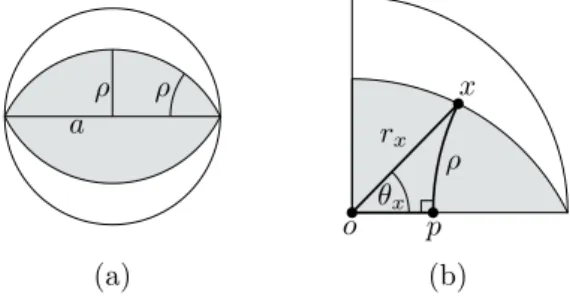
ρ ρ a ρ o rx x θx p (a) (b)
Figure 1(a) The hyperdisk (gray) with radiusρand horizontal axisagoing through the origin. (b) A right triangle in the hyperbolic plane.
Separator Hierarchy. Let Dbe a metric space (e.g., a disk in hyperbolic space or a graph). Aseparator hierarchy ofDis a rooted treeT with tnodes where each nodeiis associated with a subset Si ∈ D such that S = {S1, . . . , St} partitions D, i.e., D = SSi∈SSi and
Si∩Sj =∅ for i=6 j. For every nodei, let Ui =Si∪
S
j∈desc(i)Sj, where desc(i) are the
descendants ofiin T. For (T,S) to be a separator hierarchy, we require that for every pair of sibling nodesiandj(i.e., nodes with the same parent) the setUi is disconnected fromUj. For the parentkofiand j, we also say thatSk is theseparator that separatesUi fromUj.
Thediameter of the separatorSk (separatingUi andUj) is the largest valuedsuch that
every element inUi has distance at leastdform every element inUj. The diameter of the
separator hierarchy (T,S) is the minimum diameter of all its separators. For a given measure
µonD, the separatorSk is balanced ifµ(Ui)≤1/2µ(Uk) andµ(Uj)≤1/2µ(Uk). If these
inequalities hold in expectation, we say thatSk is expected to be balanced. The separator hierarchy is balanced (in expectation) if each separator is balanced (in expectation).
Treewidth. LetT be a tree witht nodes and letX ={X1, . . . , Xt}be a family of sets. For each nodeiofT, the setXi is called thebag ofi. The pair (T,X) is atree decomposition of
a graphG= (V, E) if the bags are subsets ofV satisfying the following two properties.
(i) For each vertexv∈V, the nodes ofT whose bags containv induce a subtree ofT.
(ii) For each edge uv∈E, there exist a bag X∈ X withu∈X andv∈X.
Thewidthof a tree decomposition is the size of the largest bag minus 1. Thetreewidthtw(G) of a graphGis the smallestk for whichGhas a tree decomposition of widthk.
3
Hyperdisk Decomposition
In this section, we define a separator hierarchy for a diskD in the hyperbolic plane. We assume thatD is centered at the origin. The separators are (parts of) hyperdisks, which are defined as follows. Letabe a line in the hyperbolic plane. The set of points with distanceρ
fromaform thehypercirclewithradiusρandaxisa. The set of points with distance at most
ρfromais the corresponding hyperdisk; see1 Fig. 1a. We usually consider lines through the origin as axes. Byaγ, we denote such a line whose points have angleγ orγ+π.
Letx= (rx, θx) be a point on the hypercircle with axis a0 and radius ρ. Moreover, let o
be the origin and letpbe the point onaγ such that the line throughxandpis perpendicular
toaγ. Theno, p, andxform a triangle with right angle atp; see Fig. 1b. The angle ato
1 We use the Poincaré disk model in illustrations. Thus, the disk shown in Fig. 1 (as well as the outer-most
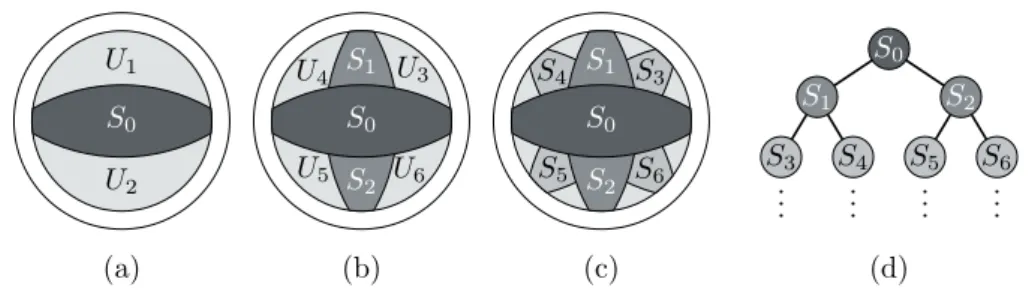
S0 U1 U2 S0 S1 S2 U3 U4 U5 U6 S0 S1 S2 S3 S4 S5 S6 S0 S3 S6 S2 S5 S4 S1 .. . ... ... ... (a) (b) (c) (d)
Figure 2(a) The diskD(gray area) is separated byS0 (dark gray) into the two regionsU1and
U2 (light gray). (b, c) The separators on levels 1 and 2. (d) The corresponding separator hierarchy
represented as tree in which each node corresponds to a separator.
isθx, the length of the opposite side xpisρ, and the length of the hypotenuse isrx. The
trigonometry of hyperbolic right triangles yields the following equation, which we need later. sin(θx) = sinh(ρ)
sinh(rx)
(2) The hyperdisk decomposition of D is the following separator hierarchy. The top-level separator (level 0)S0 is the intersection ofDwith the hyperdisk with axisa0 (all hyperdisks we consider have arbitrary but fixed radiusρ). This symmetrically separatesD into regions
U1 andU2 above and belowS0; see Fig. 2a. The region U1 (and analogouslyU2) is again symmetrically separated into two parts by its intersection with the hyperdisk with axisaπ/2. Denote the resulting separator byS1and the two separated regions byU3andU4; see Fig. 2b. On the next level,U3 (and analogouslyU4, . . . , U6) is separated by its intersection with the hyperdisk with axisaπ/4 ; see Fig. 2c. We continue this decomposition untilSi=Ui. Clearly, this leads to a separator hierarchy (T,S) andT is a complete binary tree; see Fig. 2d.
3.1
Properties of the Hyperdisk Decomposition
In the following, we investigate different properties of the hyperdisk decomposition, depending on the radiusRof the diskD, on the radiusρof the hyperdisks, and on a measureµonD. We start with two simple observations. The first observation follows from the fact that two points on different sides of a hyperdisk with radiusρhave distance at least 2ρ(they have distanceρfrom the hyperdisk’s axis and the line segment connecting them crosses the axis). IObservation 2. The hyperdisk decomposition has diameter at least2ρ.
We will later set ρ=R/2 (Section 3.2) or to something even larger (Section 6). However, the bounds we prove in this section hold for more general choices ofρ.
The next observation follows from the fact that for two nodes iandj on the same level, the regionsUi andUj are symmetric with respect to rotation around the origin.
IObservation 3. The hyperdisk decomposition is balanced for every measure that is invariant under rotation around the origin.
The measure we are particularly interested in isµgiven byµ(S) =R
Sf(r) drwith the
density function f(r) as defined in Equation (1). Note that µ is clearly invariant under rotation around the origin as f does not depend on the angle of a given point. In the remainder of this section, we always assumeµto be this measure.
Our main goal in the following is to bound the measure of the separators in the hyperdisk decomposition. Clearly, the measure of the separators decreases for increasing level. To quantify this, we first show the following lemma.
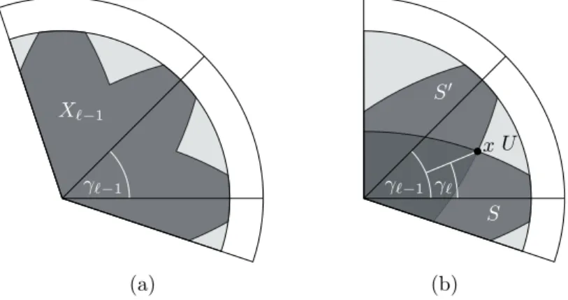
γ`−1 U S S0 x γ`−1 γ` X`−1 (a) (b)
Figure 3(a) The regionX`−1. (b) Two consecutive hyperdisks enclosing the regionU.
ILemma 4. Let S be a separator on level `≥ 1 of the hyperdisk decomposition and let
x∈S be a point with radiusrx. Then the following holds:
rx≥rmin= max{ρ, ρ+ log(1−e−
2ρ)−log(22−`−22−2`)}.
Proof. We show that the inequality holds for every pointxthat is not contained in a separator of level less than`. Clearly,rx≥ρholds as every point with smaller radius is contained in the top-level separator. It remains to showrx≥ρ+ log(1−e−2ρ)−log(22−`−22−2`).
First assume`= 1. In this case log(22−`−22−2`) = 0. Moreover, log(1−e−2ρ)<0. Thus
the claim is weaker thanrx≥ρ, which we already proved above. We assume in the following that`≥2, which implies that there are at least two separators with level less than`.
Letγ` =π/2` and consider all hyperdisks that have an axis whose angle is a multiple
ofγ`−1. LetX`−1 be the union of these hyperdisks; see Fig. 3a. By the definition of the hyperdisk decomposition, the union of all separators of level less than`equals X`−1. We show that all points not inX`−1 (and thus all points in a separator of level`) satisfy the claimed inequality. To this end, first note that rotating the discD by a multiple of γ`−1 around the origin mapsX`−1 to itself. Thus, it suffices to prove the claim for points with angles between 0 andγ`−1.
LetS andS0 be the hyperdisks whose axes have angles 0 and γ`−1, respectively, letU be the region between them, and letxbe the point whereS,S0, and U touch; see Fig. 3b. In the following we first show that actually no point inU has radius smaller thanx(which is intuitively true when looking at Fig. 3a). Afterwards it remains to show the claimed lower bound for the pointx.
Let y ∈ U be a point with coordinates (ry, θy) and let ρy be the distance of y from
the horizontal axisa0. By Equation (2), we have sinh(ρy) = sinh(ry) sin(θy). Thus, for all
relevant anglesθy, the distanceρy is increasing with increasing radius and with increasing
angle. Hence, in caseθy≤θx, the assumptionry< rximplies thatρy< ρ(recall thatρis
the distance ofxfrom the horizontal axis). Thus, y is contained in the hyperdisk S and cannot be contained inU. Symmetrically, ifθy ≥θx andry< rx, theny is contained inS0.
Hence, no point inU has smaller radius thanx.
It thus remains to show the claimed inequality for the pointx. Note thatxhas the angle
θx=γ`. Thus, by Equation (2), we have the following.
sin(γ`) =
sinh(ρ) sinh(rx)
⇔ sinh(rx) = sinh(ρ) sin(γ`) ⇔ erx−e−rx= e ρ−e−ρ sin(γ`) ⇒ erx≥ e ρ−e−ρ sin(γ`) ⇔ rx≥log(eρ−e−ρ)−log(sin(γ`)) =ρ+ log(1−e−2ρ)−log(sin(γ`))
We use that sin(γ)≤1−(1−2/π·γ)2 forγ∈[0, π/2] to obtain the following. sin(γ`)≤1− 1− 2 πγ` 2 = 1−1−21−` 2 = 22−`−22−2`
Together with the previous inequality, this yields the claimed bound. J The above lemma together with a simple calculation shows the following. With the height of the hyperdisk decomposition (which is a separator hierarchy), we refer to the height of the corresponding tree, i.e., to the maximum distance from a node to the root.
ILemma 5. The hyperdisk decomposition has height O(R) ifρ≥εfor a constantε.
Proof. We show that setting`= log2(c·eR) + 2 =O(R) (for a suitable constantc) results in
rmin≥R. Thus, the separators with smaller levels already cover the whole disk of radiusR. The last part of the formula given forrmin in Lemma 4 can be rewritten as follows.
−log22−`−22−2`≥ −log22−`= log2`−2= log(c) +R
When choosing c= (1−e−2ε)−1, Lemma 4 yieldsr
min≥R. J
In the following, we upper bound the measure of a separator Son level`of the hyperdisk decomposition. LetH be the hyperdisk corresponding toS. To simplify the calculations, we rotate the disk such thata0 (i.e., the horizontal line through the origin) is the axis ofH. First assume that`≥1 and letrminbe the lower bound for the radius shown in Lemma 4. Consider the setS0 of all points inH with radius at leastrmin that lie to the right of the origin (angle between−π/2 andπ/2). ClearlyS⊆S0 and thusµ(S)≤µ(S0).
To computeµ(S0), letθρ(r) be the angle between 0 andπ/2 such that the point (r, θρ(r))
lies on the hypercircle boundingH. By Equation (2), we haveθρ(r) = arcsin(sinh(ρ)/sinh(r)).
We obtain the following (recall thatf(r) is the density function).
µ(S0) = Z S0 f(r) dr= R Z rmin θρ(r) Z −θρ(r) f(r) dθdr= R Z rmin 2θρ(r)f(r) dr (3)
Note thatθρ(r) is only well-defined ifr≥ρ. For`≥1, this is not an issue asrmin≥ρby Lemma 4. However, the case thatS =H is the top-level separator needs special treatment. In this case, we partitionS into the diskDρ of radiusρand the subsets S0 andS00 of H
whose points have radius at leastρand lie to the right and left of the origin, respectively. Due to symmetry, µ(S0) = µ(S00). Thus,µ(S) = µ(Dρ) + 2µ(S0). Gugelmann et al. [18]
showed thatµ(Dρ) =e−α(R−ρ)(1 +o(1)). Moreover, forµ(S0) we again obtain Equation (3)
withrmin=ρ. We thus obtain the following lemma by bounding µ(S0) from above. Note that we requireρto be linear inRhere.
ILemma 6. Let S be a separator on level ` of the hyperdisk decomposition of DR with
hyperdisks of radiusρ∈Ω(R). Then the following holds.
µ(S) = O eαρ−αR· 21−α−` forα <1 O eρ−R·R forα= 1 O eρ−R forα >1
Proof. For the special case`= 0,µ(Dρ) =O(eαρ−αR) is dominated by the claimed bounds
for all α. Thus, for all cases, it remains to prove the bounds for µ(S0). Starting with Equation (3) and using that arcsin(x)≤x·π/2 (forx≥0), we get the following.
R Z rmin 2θρ(r)f(r) dr≤ R Z rmin 2·π 2 · sinh(ρ) sinh(r) · α 2π · sinh(αr) cosh(αR)−1dr =α 2 · sinh(ρ) cosh(αR)−1· R Z rmin sinh(αr) sinh(r) dr =α 2 · sinh(ρ) cosh(αR)−1· R Z rmin eαr−e−αr er−e−r dr =α 2 · sinh(ρ) cosh(αR)−1· R Z rmin er er−e−r · eαr−e−αr er dr ≤α 2 · sinh(ρ) cosh(αR)−1· eρ eρ−e−ρ · R Z rmin eαr er dr =Oeρ−αR· R Z rmin e(α−1)rdr
The last inequality follows from the facts that er
er−e−r is monotonically decreasing (and thus maximal forr=rmin≥ρ) and thate−αr is positive. In caseα= 1, the integral equals to
R−rmin≤R, yieldingµ(S0) =O(eρ−R·R). Otherwise, we have the following. R Z rmin eαr er dr= " e(α−1)r α−1 #R rmin = e (α−1)R−e(α−1)rmin α−1
Ifα >1, the integral is dominated bye(α−1)R, yieldingµ(S0) =O(eρ−αR·eαR−R) =O(eρ−R).
Ifα <1, the integral is dominated bye(α−1)rmin. Using the bound forr
mingiven by Lemma 4, we obtain the following.
µ(S0) =Oeρ−αR·e(α−1)rmin
=Oeρ−αR·e(α−1)ρ·1−e−2ρ
α−1
·22−`−22−2` 1−α
In this product, the first two factors simplify toO(eαρ−αR). The third factor tends to 1 for increasingρ(and ρ∈Ω(R)). The fourth factor can be written as 2−`(1−α)(22−22−`)1−α.
3.2
Decomposing Hyperbolic Random Graphs
Recall that one obtains a hyperbolic random graphGby randomly placingnvertices in the diskD of radiusR = 2 logn+C according to the probability measureµ and connecting two vertices if and only if their distance is less thanR. For a subsetS ⊆D, letG[S] be the subgraph ofGinduced by vertices inS.
Let (T,S) be the hyperdisk decomposition ofD with hyperdisks of radiusρ=R/2. Let further k be a node of T with children i and j. By Observation 2, the diameter of the separatorSk (separatingUi fromUj) is at least 2ρ=R. This implies that no vertex inUiis
connected to a vertex inUj. Thus, the graphG[Uk] is separated by the vertices inSk into
the subgraphsG[Ui] andG[Uj]. Hence, the hyperdisk decomposition ofD translates into
a separator hierarchy of the graph G. We also call this separator hierarchy thehyperdisk decompositionofG. The properties of the separators inDdirectly translate to the separators inG, i.e., we can expect the separators to be balanced (Observation 3) and small (Lemma 6). ITheorem 7. The hyperdisk decomposition of a hyperbolic random graph is expected to be balanced and for a separatorS on level`, the following holds.
E|S|= O n1−α · 21−α−` forα <1 O(logn) forα= 1 O(1) forα >1
4
The Treewidth of Hyperbolic Random Graphs
The treewidth of a graphGis closely related to the size of separators inG. IfGhas treewidth
k, it is known to have a balanced separator of sizek+ 1. This follows from the fact that a tree (e.g., the decomposition tree of widthk) has a (weighted) balanced separator of size 1. Conversely, ifGcan be recursively decomposed by small balanced separators, i.e., if it has a balanced separator hierarchy with small separators, its treewidth is also small.
The following statement is easy to prove and for example used to show that planar graphs have treewidth√nbased on the planar separator theorem.
ILemma 8. Let(T,S)be a separator hierarchy ofG. For each nodeiofT, letXibe the union
ofSi and all separatorsSj for whichj is an ancestor ofi inT. Then (T,X ={X1, . . . , Xt})
is a tree decomposition ofG.
Proof. We have to show that for each vertexv∈V the bags containingv form a subtree of
T and that for each edgeuv∈E, there exists a bag containinguandv. For the former, let
v be a vertex and letibe the unique node ofT such thatv∈Si. Thenv∈Xj if and only if
j=iorj is an descendant ofi. The nodeitogether with its descendants clearly is a subtree ofT. For the second condition, letuv∈E, letu∈Si andv∈Sj. Due to their edge,uand
v cannot be separated, which implies thatiis an ancestor ofj or vice versa. Without loss of generality, we assumeiis an ancestor ofj. Then Xj includes Sj and Si, which proves the
claim. J
Using the properties of the hyperdisk decomposition as stated in Lemma 5 and Theorem 7 together with Lemma 8, we obtain a tree decomposition with upper bounds on the expected size of each bag. Applying a Chernoff bound (Theorem 1) leads to the following theorem.
ITheorem 9. For the treewidthtw(G)of a hyperbolic random graph G, the following holds with high probability.
tw(G) = Θ n1−α forα <1 Olog2n forα= 1 O(logn) forα >1
Note that the theorem states a matching lower bound ifα <1. It follows from the fact that hyperbolic random graphs have clique number Θ(n1−α) ifα <1 [14]. Forα≥1, the
clique number is Θ(logn/log logn) [14]. Thus, our upper bounds forα= 1 andα >1 differ from this lower bound by factors lognlog lognand log logn, respectively.
5
Applications
Our results from the previous sections have several algorithmic implications. In particular, the logarithmic treewidth forα >1 leads to efficient algorithms for numerous NP-hard problems, e.g.,Vertex Cover, Independent Set, Dominating Set, Odd Cycle Traversal, andMax Cut[9]. We note that the size of the largest connected component in a hyperbolic random graph is whp polynomial even forα > 1 as the maximum degree [18] is a lower bound for the size of the largest component. Thus, for α >1, the treewidth is not only logarithmic in the size of the whole (potentially disconnected) hyperbolic random graph but also in the size of the largest component.
Forα <1, the separators are larger and thus algorithmic applications are less obvious. Moreover, there exists agiant component [3], i.e., a connected component of linear size. In the following sections, we present several algorithmic applications for the case thatGis the giant component of a hyperbolic random graph withα <1. We note that all results still hold when considering the whole hyperbolic random graph instead of only the giant component (in fact, some arguments actually get simpler).
We give an approximation scheme forIndependent Set(Section 5.1) and a fast algorithm for computing maximum matchings (Section 5.2). Both results assume that the geometry of the hyperbolic random graph is known (which is a strong but not completely unreasonable assumption [4]). In Section 5.3 we give applications that do not rely on knowing the geometry.
5.1
An Approximation Scheme for Independent Set
As an independent set forms a clique in the complement graph and vice versa, it is NP-hard to approximateIndependent Setwith approximation ratio better than O(n1−ε) for any
ε >0 [30]. However, based on the planar separator theorem (stating that planar graphs have balanced separators of sizeO(√n)), Lipton and Tarjan [25] showed that Independent Seton planar graphs has aPTAS (polynomial-time approximation scheme), i.e., for every constantε >0, it admits an efficient approximation algorithm with approximation ratio 1−ε. We adapt their approach to show that there is an approximation scheme forIndependent Setif the input is a hyperbolic random graph given in its geometric representation.
The PTAS for planar graphs is based on two facts. First, planar graphs have a balanced separator hierarchy with separators of sizeO(√n). Second, planar graphs have independent sets of linear size. The latter follows directly from the fact that planar graphs have bounded chromatic number. For hyperbolic random graphs, this is not true, as they include com-paratively large cliques [14]. However, as the degree sequence follows a power law, we find
a subgraph of linear size whose vertices have bounded degree. This subgraph can then be colored with a constant number of colors which implies a large independent set. To obtain the following lemma, we have to apply this argument to the giant component of a hyperbolic random graph.
ILemma 10. The giant component of a hyperbolic random graph has whp independent sets of linear size.
Following the approach of Lipton and Tarjan [25], we prove the following lemma. The rough idea is to chooseV0 to be the union of all separators of the hyperdisk decomposition with level at mostblog2(n/k)c.
ILemma 11. LetG= (V, E)be a hyperbolic random graph withα <1and letk∈N. Then there is a vertex set V0⊆V of expected size O(n)/kα such that the connected components of
G−V0 have expected size at mostk.
Proof. Consider the hyperdisk decomposition (T,S) of Gand let i be a node on level `. Recall thatUidenotes the set of vertices such thatG[Ui] is the subgraph whose separators are
represented by the descendants ofiin T. Due to the fact that the hyperdisk decomposition is balanced (Theorem 7), the expected size ofUi is at mostn2−`. We chooseV0 to be the
union of all separators with level at most`max=blog2(n/k)c. Each connected component of
G−V0 is then a subgraph ofG[Ui] for a vertexiwith level `max+ 1. Thus, the expected size of these components is at mostk.
It remains to boundE[|V0|]. Recall from Theorem 7 that a separator on level`has expected sizeO(n1−α)·2−`(1−α). Moreover, asT is a complete binary tree, there are 2` separators on level`. Thus, the total size of separators on level`isO(n1−α)·2−`(1−α)2`=O(n1−α)·2α`.
We thus obtain the following for the expected size ofV0.
E|V0|= `max X `=0 On1−α·2α` =On1−α· `max X `=0 2α`
To conclude the proof, it remains to proof that the sum equals (n/k)α·O(1), which follows
from the following calculation and from the fact that the geometric series converges.
`max X `=0 2α`= `max X i=0 2α(`max−i) = 2α`max `max X i=0 2−αi = n/kα ·O(1) J
To approximate Independent Set, one can apply Lemma 11 to the given hyperbolic random graphGand then compute for each of the resulting connected components an optimal independent set in expected time O(k2k). For allO(n/k) connected components, this takes
expectedO(n2k) time. The union of these independent sets is an independent set ofG. Let
I be this independent set, restricted to the giant componentH ofG. Comparing this to the size of an optimal independent setI? ofH, we miss at most the vertices in the separatorV0,
thusE[|I?| − |I|] =O(n)/kα. As|I?|is linear with high probability (Lemma 10), dividing by|I?|yields
E[1− |I|/|I?|] =k−α·O(1) and thusE[|I|/|I?|] = 1−k−α·O(1).
This directly implies the claimed approximation scheme: for every givenε >0, one can choose thek such that the expected approximation ratio is 1−ε. As thekwe have to chose does not depend onn, the resulting running time is polynomial inn(but exponential in 1/ε). Additionally applying concentration bounds ifk= lognyields the following theorem. I Theorem 12. For the giant components of hyperbolic random graphs given in their geometric representation,Independent Set can be approximated in expected O(n2k)time with expected approximation ratio1−k−α·O(1). Ifk= logn, the algorithm runs whp in
polynomial time and the bound on the approximation ratio holds whp.
Proof. It remains to consider the casek= logn. We apply Lemma 11 withk= lognleading to connected components of expected size logn. Using a Chernoff bound (Theorem 1) shows that the size of the connected components is whp at mostclognfor a constantc. Thus, the algorithm described above has whp polynomial run-time.
Concerning the approximation ratio, note that the separator V0 has expected size
O(n)/logαn. Thus, there are constants c1 and nmin such that the E[|V0|] ≤c1n/logαn ifn > nmin. As we can brute-force smaller instances, we can assume the latter assump-tion to be true. Applying a Chernoff bound (Theorem 1) we get that V0 includes whp at mostc2n/logαn vertices for another constant c2. As before let I be the independent set we computed and letI? be an optimal independent set of the giant component. Then,
|I?| − |I| ≤c
2n/log
αnholds whp. As whp|I?| ≥c
3n(at least for sufficiently large instances; see Lemma 10), the calculations from above show that|I|/|I?| ≥1−c/logαnholds whp for
c=c2/c3. J
5.2
Computing Matchings in
O
(
n
2−α)
Time
Lipton and Tarjan [25] also gaveO(n3/2) andO(n3/2logn) algorithms that compute match-ings of maximum cardinality and matchmatch-ings of maximum weight, respectively, in a planar graph. Their algorithm uses the following divide-and-conquer strategy. Find a separator, recursively compute maximum matchings for both subgraphs, and finally combine these solutions by iteratively adding the vertices of the separator while maintaining a maximum matching. The latter can be done by finding a single augmenting path, which can be done inO(m) andO(mlogn) time for unweighted and weighted graphs, respectively (mis the number of edges).
To obtain the following theorem, we apply this divide-and-conquer strategy to hyperbolic random graphs, show thatm is actually linear inn(even for the subgraphs for which we compute the augmenting paths), and apply concentration bounds.
ITheorem 13. Let Gbe the giant component of a hyperbolic random graph given in its geometric representation. Whp, a maximum matching inGcan be computed inO(n2−α)and
O(n2−αlogn)time if Gis unweighted and weighted, respectively.
5.3
In Case the Geometry is Unknown
The two previous applications relied on the fact that we know the geometric representation of the given hyperbolic random graph. However, even if the geometry is unknown, we can still benefit from the knowledge that hyperbolic random graphs have low treewidth by using an algorithm of Fomin et al. [13]. It takes a graphGand an integerkas input and either decides that tw(G)> kor returns a tree decomposition of widthk2. It runs inO(k7nlogn)
time. By spending an additional factor of log(tw(G)) we can actually compute the smallest
kfor which the algorithm succeeds to compute a tree decomposition.
Given a tree decomposition of widthk, Fomin et al. [13] show (among other algorithms) how to compute a matching with maximum weight and a maximum vertex flow in a directed graph inO(k4nlog2n) andO(k2nlogn) time, respectively. For sufficiently largeα, this leads to algorithms solving these problems faster than the best known algorithms for general graphs. E.g., forα= 31/32, the treewidth ofGisO(n1/32) with high probability (Theorem 9). Thus, we get a tree decomposition of width O(n1/16) in O(n7/32·nlog2n) time. Computing a matching of maximum weight then takesO(n1/4·nlog2n). Thus, the overall running time is O(n5/4log2n). Also note that this approach leads to almost linear (i.e., linear up to a polylogarithmic factor) run-times ifα≥1.
6
Binomial Hyperbolic Random Graphs
So far, we considered the so-called threshold model of hyperbolic random graphs where vertices are connected if and only if they have distance at mostR. A more realistic (but technically more difficult) model is thebinomial model, in which longer edges and shorter non-edges are allowed with a certain probability. More precisely, two vertices with distance
dare connected with the following probability p(d) depending on the constantt (usually 0< t <1). Note that we obtain the threshold model fort→0.
p(d) =1 +e21t(d−R)
−1
As before, we start with a hyperdisk decomposition (T,S) of the diskDand then transfer it to a separator hierarchy of a hyperbolic random graph. In the threshold model, separators in (T,S) translated to separators in the graph ifρ≥R/2. This is not true in the binomial model as vertices with distance greater thanRare still connected with a certain probability.
However, we obtain separators as follows. Let kbe a node of T with childreniandj, i.e.,Sk separatesUk intoUi andUj. An edge of the graphGiscritical with respect toSk if
it connects a vertex located in Ui with a vertex in Uj. As before, letG[Uk] be the graph induced by vertices in Uk. Then the vertices located in Sk together with the endvertices
of critical edges separateG[Uk] into (subgraphs of)G[Ui] andG[Uj]. In this way, we again
obtain a separator hierarchy forG, which we call theextended hyperdisk decomposition. To bound the size of the resulting separators, we have to bound the number of vertices inSk and the number of critical edges. For the former, we can use the previous results (in
particular Lemma 6). For the latter, note that the expected number of vertices inUi is at
mostn2−`ifihas level`(as the hyperdisk decomposition is balanced). As the same holds
forUj, there are only (n2−`)2 vertex pairs that potentially form critical edges, each with a
probability of at mostp(2ρ) (as their distance is at least 2ρ). Thus, the expected number of critical edges is at most n2p(2ρ)2−2`. Plugging a carefully chosen value forρinto this formula as well as into the formula given by Lemma 6 leads to the following theorem. ITheorem 14. LetGbe a binomial hyperbolic random graph withα <1and consider its extended hyperdisk decomposition with hyperdisks of radiusρ= 2αt2αt++2t+1R. For a separatorS
on level`, the following holds. E(|S|) =O n2−αtα+1+1 ·21−α −`
Proof. As mentioned above, the number of critical edges is bounded by the following term.
n2p(2ρ)2−2`=n2p
2αt+t+ 1
αt+ 1 R
=n21 +e21t( 2αt+t+1 αt+1 R−R) −1 2−2` =n21 +e12 α+1 αt+1R −1 2−2` =n21 +e12 α+1 αt+1(2 logn+C) −1 2−2` ≤n21 +eαtα+1+1(logn+C/2) −1 2−(1−α)` =On2−αtα+1+1 ·21−α −`
For the second part, we go one step back and assume thatSis a separator in the hyperdisk decomposition of the diskDRin the hyperbolic plane (instead of a separator in graph). By
Lemma 6, we get the following bound on the measure ofS.
µ(S) =Oeαρ−αR 21−α −` =Oeα2αt2αt++2t+1R−αR 21−α −` =Oeα2αtt−+21 R 21−α −` =Oeα2αtt−+21 (2 logn+C) 21−α −` =Onαtαt−+1α 21−α −` =Onαt+1αt−+1α−1 21−α −` =On1−αtα+1+1 21−α −`
Multiplying withn(as we havenvertices) leads to the claimed bound. J Note that this bound coincides with our result for the threshold model when t → 0. Moreover, fort∈(0,1), we obtain separators of sublinear size. As for the threshold model, we can use Lemma 8 to obtain bounds for the treewidth (compare Section 4).
7
Conclusion
We have shown that hyperbolic random graphs have small separators, as well as a small treewidth (with a phase transition from polynomial to logarithmic atβ= 3). This stands in stark contrast to other popular random graph models like Erdős-Rényi [12] or Barabási-Albert [2] that have linear separators [17]. Beyond providing new insights on the structural properties of hyperbolic random graphs, our results give rise to several algorithmic applica-tions.
To judge the practical merit of these algorithms, an interesting next step is therefore to compare separators on real graphs with predictions made by the various models. It is, however, a challenge to compute small separators in a given massive graph. Depending on the precise problem formulation, this is likely to be an NP-complete problem.
A more theoretical open question is whether our results are tight or can be improved to achieve even smaller separators. Of interest is especially the binomial model, since it allows for long range edges in the graph; and there exists no lower bound on the treewidth in the current literature.
References
1 Mohammed Amin Abdullah, Michel Bode, and Nikolaos Fountoulakis. Typical distances in a geometric model for complex networks. CoRR, abs/1506.07811:1–33, 2015.
2 Albert-László Barabási and Réka Albert. Emergence of scaling in random networks.Science, 286(5439):509–512, 1999.
3 Michael Bode, Nikolaos Fountoulakis, and Tobias Müller. On the largest component of a hyperbolic model of complex networks. The Electronic Journal of Combinatorics, 22(3):1– 46, 2015.
4 Marián Boguñá, Fragkiskos Papadopoulos, and Dmitri Krioukov. Sustaining the internet with hyperbolic mapping. Nature Communications, 1(62), 2010.
5 Béla Bollobás and Oliver M. Riordan. Mathematical Results on Scale-Free Random Graphs, chapter 1, pages 1–34. Wiley, 2005.
6 Karl Bringmann, Ralph Keusch, and Johannes Lengler. Geometric inhomogeneous random graphs. CoRR, abs/1511.00576:1–42, 2015.
7 Fan Chung and Linyuan Lu. The average distance in a random graph with given expected degrees. Internet Mathematics, 1(1):91–113, 2003.
8 Aaron Clauset, Cosma Rohilla Shalizi, and M. E. J. Newman. Power-law distributions in empirical data. SIAM Review, 51(4):661–703, 2009.
9 Marek Cygan, Fedor V. Fomin, Łukasz Kowalik, Daniel Lokshtanov, Daniel Marx, Marcin Pilipczuk, Michał Pilipczuk, and Saket Saurabh. Parameterized Algorithms. Springer International Publishing, 2015.
10 Rodney G. Downey and Michael R. Fellows. Parameterized Complexity. Springer-Verlag New York, 1999.
11 Devdatt P. Dubhashi and Alessandro Panconesi.Concentration of Measure for the Analysis of Randomized Algorithms. Cambridge University Press, 2012.
12 P. Erdős and A. Rényi. On random graphs. I. Publicationes Mathematicae, 6:290–297, 1959.
13 Fedor V. Fomin, Daniel Lokshtanov, Michał Pilipczuk, Saket Saurabh, and Marcin Wrochna. Fully polynomial-time parameterized computations for graphs and matrices of low treewidth. CoRR, abs/1511.01379:1–44, 2015.
14 Tobias Friedrich and Anton Krohmer. Cliques in hyperbolic random graphs. InProceedings of the IEEE Conference on Computer Communications (INFOCOM’15), pages 1544–1552, 2015.
15 Tobias Friedrich and Anton Krohmer. On the diameter of hyperbolic random graphs. In Proceedings of the 42nd International Colloquium on Automata, Languages, and Program-ming (ICALP’15), pages 614–625, 2015.
16 Yong Gao. On the threshold of having a linear treewidth in random graphs. In Pro-ceedings of the 12th Annual International Conference on Computing and Combinatorics (COCOON’06), pages 226–234, 2006.
17 Yong Gao. Treewidth of Erdős-Rényi random graphs, random intersection graphs, and scale-free random graphs. Discrete Applied Mathematics, 160(4–5):566–578, 2012.
18 Luca Gugelmann, Konstantinos Panagiotou, and Ueli Peter. Random hyperbolic graphs: Degree sequence and clustering. In Proceedings of the 39th International Colloquium on Automata, Languages, and Programming (ICALP’12), pages 573–585, 2012.
19 Michał Karoński, Edward R. Scheinerman, and Karen B. Singer-Cohen. On random in-tersection graphs: The subgraph problem. Combinatorics, Probability and Computing, 8(1–2):131–159, 1999.
20 Marcos Kiwi and Dieter Mitsche. A bound for the diameter of random hyperbolic graphs. InProceedings of the 12th Workshop on Analytic Algorithmics and Combinatorics (ANALCO’15), pages 26–39, 2015.
21 Dmitri Krioukov, Fragkiskos Papadopoulos, Maksim Kitsak, Amin Vahdat, and Marián Boguñá. Hyperbolic geometry of complex networks. Physical Review E, 82:036106, 2010.
22 Choongbum Lee, Joonkyung Lee, and Sang il Oum. Rank-width of random graphs.Journal of Graph Theory, 70(3):339–347, 2012.
23 Anshui Li and Tobias Müller. On the treewidth of random geometric graphs and percolated grids. Manuscript, 2015.
24 Richard J. Lipton and Robert E. Tarjan. A separator theorem for planar graphs. SIAM Journal on Applied Mathematics, 36(2):177–189, 1979.
25 Richard J. Lipton and Robert E. Tarjan. Applications of a planar separator theorem.SIAM Journal on Computing, 9(3):615–627, 1980.
26 Silvio Micali and Vijay V. Vazirani. Ano(p|V||e|) algorithm for finding maximum match-ing in general graphs. InProceedings of the 21st Annual Symposium on Foundations of Computer Science (FOCS’80), pages 17–27, 1980.
27 Dieter Mitsche and Guillem Perarnau. On the treewidth and related parameters of ran-dom geometric graphs. InProceedings of the 29th International Symposium on Theoretical Aspects of Computer Science (STACS’12), pages 408–419, 2012.
28 Fragkiskos Papadopoulos, Dmitri Krioukov, Marián Boguñá, and Amin Vahdat. Greedy forwarding in dynamic scale-free networks embedded in hyperbolic metric spaces. In Pro-ceedings of the 29th Conference on Information Communications (INFOCOM’10), pages 2973–2981, 2010.
29 Remco van der Hofstad. Random graphs and complex networks. Vol. II.http://www.win. tue.nl/~rhofstad/NotesRGCNII.pdf, 2014.
30 David Zuckerman. Linear degree extractors and the inapproximability of max clique and chromatic number. In Proceedings of the 38th Annual ACM Symposium on Theory of Computing (STOC’06), pages 681–690, 2006.