Optimal operations of transportation fleet for unloading activities at container ports

(1)

Optimal operations of transportation ﬂeet

for unloading activities at container ports

Seungmo Kang, Juan C. Medina, Yanfeng Ouyang

*

Department of Civil and Environmental Engineering, University of Illinois at Urbana-Champaign, Urbana, IL 61801, USA Received 3 March 2007; received in revised form 9 February 2008; accepted 11 February 2008

Abstract

This paper presents mathematical models that optimize the size of transportation fleet (cranes and trucks) for unloading operations at container terminals. A cyclic queue model is used to study the steady-state port throughput, which then yields the optimum fleet size for long-term operations. This model allows for stochastic operations such as exponentially distributed crane service times. In order to allow for generally distributed crane service times and truck travel times, an approach based on Markovian decision process is also proposed. This model provides dynamic operational policies for fleet management. Both models are implemented and examined with empirical data from the Port of Balboa, Panama. These models are also extended to unloading operations that involve multiple berths.

Published by Elsevier Ltd.

Keywords: Container terminal; Unloading operation; Cyclic queue model; Markovian decision process; Fleet size optimization

1. Introduction

The transportation of container cargo has become highly standardized in the intermodal shipping industry. The number of container units handled at maritime ports was estimated to have increased 55% between 1998 and 2005, to a total of 270 million 20-foot equivalent units in 2005 (The World Bank Group, 2006). Although container terminals have increased their capacity to process a greater number of containers per year, the rapid growth in container cargo volume poses a constant need for optimal use of port resources that reduces oper-ating costs and increases cargo throughput.

The handling process at container ports is quite sophisticated. In general, each container may go through one or more of the following four phases: loading, unloading, storage, and transfer to other ships or land based transportation services. In the unloading phase, containers are unloaded and transported from the ves-sel to the storage yard. The equipment involved generally includes quayside cranes (QC) at berths, rubber tire gantry cranes (RTGC) at storage yards, and terminal trucks (or tractors). The QCs are in charge of lifting and

0191-2615/$ - see front matter Published by Elsevier Ltd. doi:10.1016/j.trb.2008.02.003

* _{Corresponding author. Tel.: +1 217 333 9858; fax: +1 217 333 1924.}

E-mail addresses:skang2@uiuc.edu(S. Kang),jcmedina@uiuc.edu(J.C. Medina),yfouyang@uiuc.edu(Y. Ouyang). Transportation Research Part B 42 (2008) 970–984

(2)

moving containers from the vessels to the trucks. A number of trucks travel in a dedicated closed loop to pick up containers at the berth and drop them at the storage yard. Each truck usually handles one container at a time. Once the container arrives at the yard, a RTGC lifts it and stores it inside the yard premises.

Delays can occur if trucks are queued at the berth and/or the yard, depending on the number of available cranes and the arrival rate of the trucks. The unloading operation itself can be further decomposed into multi-ple stages, each of which can be studied separately. For exammulti-ple,Shields (1984)studied the most efficient order for a QC to pick up containers from a vessel, andNarasimhan and Palekar (2002)studied the transtainer rout-ing problem, which seeks the optimal sortrout-ing and stackrout-ing of containers at storage yards that minimizes oper-ating time. Goodchild and Daganzo (2006) studied a double cycling strategy for more efficient crane operations at the berth. In double cycling, containers are loaded and unloaded in the same crane cycle, poten-tially increasing the productivity and reducing the operating time per vessel. Furthermore, Goodchild and Daganzo (2007) explored the long-term benefits of a particular ‘‘proximal stack strategy” for unloading and loading containers from and to the vessels. Operating times were reported to decrease by up to 10% while using double cycling.

The literature also presents a series of optimization tools for analyzing container loading and unloading operations, mostly focusing on the throughput of a terminal in the steady state. Speciﬁc techniques include queuing theory (Koenigsberg and Lam, 1976), network formulations (Steenken et al., 1993; Chen et al., 1998; Vis et al., 2001), and heuristics (Kim and Bae, 1999; Bish et al., 2001). Cyclic queue models have been applied to similar applications since the 1960s.Gordon and Newell (1967)derived general closed-form expres-sions for the expected distribution of customers in a multiple-stages cyclic queue system. Building on this,

Koenigsberg and Lam (1976) described the problem of vessels loading and unloading liquid natural gas between two ports. More recently, Garrido and Allendes (2002)applied a simpliﬁed cyclic queue model to a case study on the Port of San Antonio, Chile. All crane service times and truck travel times are assumed to be exponentially distributed.

This paper first focuses on the planning problem of finding the optimal size of fleet (i.e., the number of QC, RTGC, and trucks) for unloading operations that suffice to unload containers with the minimum operating cost.1Results from a cyclic queue model (Gordon and Newell, 1967; Koenigsberg and Lam, 1976) are used to analyze steady-state performance of the unloading system, which are then used as a subroutine to find the optimum fleet size. The cyclic queue model assumes exponentially distributed service times and steady-state operations. It provides a simple and closed-form estimate of long-run system performance in a highly stochastic operating environment, without requiring detailed information on specific container vessels. At the operational level, the stochastic nature of unloading operations mandates that the fleet configuration reacts to changing conditions in a timely manner. In this light, a Markovian decision process (MDP) model is presented as a complement of the cyclic queue model to find optimal policies for fleet management in real time. The MDP model allows for generally distributed service times and non-steady-state operations. Both models are first formulated for marine terminals with a single berth. Then the models can be used as building blocks for fleet management at terminals with multiple berths, where resources may be shared among the unloading operations of several ships.

The exposition of the paper is as follows: Section2 describes the mathematical models developed for the unloading ﬂeet operations at container terminals. Section3illustrates the results of a case study with empirical data from the Port of Balboa in the Panama Canal. Section4discusses extended models for ﬂeet management among multiple berths. Finally, Section 5provides conclusions.

2. Model formulation

In this section, we develop mathematical models that can be utilized for marine terminal fleet planning and operations. Section2.1presents a cyclic queue model to determine the steady-state performance of any terminal fleet; that performance is used to determine the optimal fleet size that minimizes cost yet satisfies

1

The reverse operation of loading containers from the storage yard to the vessel can be considered as equivalent to the unloading operation as both require the movement of the same type of cargo.

(3)

throughput requirement. Then we develop in Section2.2 a Markovian decision process framework for real-time operations.

2.1. Steady-state throughput analysis

The process of unloading vessels at container terminals can be represented by a closed loop system similar to the models inGordon and Newell (1967) and Koenigsberg and Lam (1976). The unloading process is ﬁrst decomposed into four stages, as inFig. 1: (i) the movement of an empty truck to the berth, after unloading operations at the storage yard; (ii) the process of loading a truck at the berth, which includes the truck’s wait-ing in queue (if any) at the berth; (iii) the movement of a loaded truck from the berth to the storage yard; and (iv) the process of unloading a truck at the storage yard, including RTGC service time and possible waiting time. Stage 2 QC at Berth m2 Servers µ2 µ2 µ4 µ4 QC 1 QC m2 RTGC 1 RTGC m4 µ1 µ1 µ1 * * * Stage 1 Travel Time (Yard to Berth)

N Terminal Trucks N Stage 4 RTGC at Yard m4 Servers µ3 µ3 µ3 * * * Stage 3

Travel Time (Berth to Yard) N Terminal Trucks N

…………...

……..

(4)

Suppose we havem2QC servers at the berth andm4RTGC servers at the yard, servingNtrucks that cycle

along the system. The trucks are considered as the customers of the cyclic queue system. Stages 1 and 3 are treated as ‘‘free ﬂow”stages, having one server per truck with service time equal to the travel time between stages 2 and 4.

We assume that the service time at each server is equal to 1/li, whereliis the service rate per unit time at a

server in stagei= 1, 2, 3, 4. We also assume that the service times at all servers follow negative exponential distributions. Letn1,n2,n3,n4be the number of trucks at stages 1, 2, 3, and 4 in the steady state, respectively,

andX¼ ðn1;n2;n3;n4Þ:P4_i_¼1ni¼N;niP0;integer8i

n o

be the state space of truck distribution at any time. According toGordon and Newell (1967) and Koenigsberg and Lam (1976), the probability for the system to be in state (n1,n2,n3,n4) is given by the following expression:

Pðn1;n2;n3;n4Þ ¼ ½X1 n1_½X 3 n3 n1!n3! ½X2 n2_½X 4 n4 l2l4 Pð0;N;0;0Þ 8ðn1;n2;n3;n4Þ 2X; ð1Þ whereXi¼l_l2 i 8i, andli¼ mi!minimi; if ni>mi ni!; if ni6mi

. The expected number of trucks at stageiis

ni:¼

X

niPðn1;n2;n3;n4Þ; i¼1;2;3;4; ð2Þ

and the marginal probability that exactlyrof theNtrucks are in stageiis

PN_iðrÞ:¼X

ni¼r

XPðn1;n2;n3;n4Þ: ð3Þ

In order to measure the throughput of the system, the expected number of trucks waiting at stagei(applicable for stages 2 and 4 only) is calculated as follows:

ui:¼ X1 r¼mi ðrmiÞPNiðrÞ ¼ni X mi1 r¼0 rPN_iðrÞ miþmi X mi1 r¼0 PN_iðrÞ; i¼2;4: ð4Þ

The truck cycle time equals the total average service time at all four stages and the waiting times at stages 2 and 4. The truck cycle time divided by the number of trucks in the system corresponds to the average rate for containers to be processed. Therefore, the expected headway between two consecutive truck arrivals (i.e., re-lated to ‘‘service frequency”) is

S ¼1 N X4 i¼1 1 li þW2þW4 " # ; ð5Þ

whereWi is the expected waiting time for one truck at stagei, i.e.,

Wi:¼uiS: ð6Þ

Combining(5) and (6)we have

S ¼ 1 Nu2u4 X 4 i¼1 1 l_i; and Wi¼ ui Nu2u4 X 4 i¼1 1 l_i; i¼2;4: ð7Þ

The above formulae yield a relationship between the ﬂeet size and the average cycle time in the steady state. This is a direct measure of the long-term average throughput of the unloading system.

Very often terminals have to finish unloading containers within a given time frame (i.e., imposing a con-straint on the average cycle time or headway). The best combination of fleet that minimizes operating costs while satisfying cycle-time requirements can be obtained based on(7). Suppose that the system cost is propor-tional to the number of active cranes and trucks (running or idling), as well as the cost for having the vessel waiting during the unloading operation at the berth; i.e., one QC, RTGC, truck, and the vessel incur in a cost ofcq,cr,ct, andcw, respectively (per unit time). Assume too that the terminal needs an average container flow

of at leastD/H, whereHis the maximum available time to unloadDcontainers from a vessel. The problem for planning the optimal ﬂeet size can be formulated as follows:

(5)

Min m2;m4;N

ðcqm2þcrm4þctNþcwÞ DS

s:t: S 6H=D

m2;m4;N P0;integer

Note thatSis determined from(1)–(4) and (7), andDSis the actual time needed to unload the vessel.

2.2. Operational ﬂeet management

The above cyclic queue approach is based on two rather strong assumptions. First, it assumes exponentially distributed crane service times and truck travel times. In reality, this assumption is rarely satisfied; seeGarrido and Allendes (2002)for some discussions. Simulation of the cyclic queue system with general service time dis-tributions will address this issue. Second, the steady-state results do not apply to transient states (e.g., the beginning of an unloading process, or the unloading of a small ship). In this section, we present a Markovian decision model to optimally manage the fleet in real time; i.e., to provide guidance on how many QCs, RTGCs and trucks to operate at each specific time.

For simplicity, we aggregate stages 2, 3 into one, and 4, 1 into another.Fig. 2illustrates the operations of this aggregated two-stage system. Consider a time horizon (e.g., the time available to unload a vessel),H, in which all operations in the system (e.g., the truck travel time and crane service time) are stochastic. For any timet2[0,H], letx(t),x0₍_t_),_y₍_t_{) and}_y0₍_t_{) be the cumulative numbers of trucks that have entered service at the}

berth, arrived at the yard queue, entered service at the yard and arrived at the berth queue (after unloading a container at the yard), respectively; z(t) be the cumulative arrival of trucks available to enter service at the berth. As the number of containers is reasonably large, we assume that these cumulative values change con-tinuously with time, as illustrated by the cumulative queuing diagrams (Newell, 1982) inFigs. 3 and 4. The shaded areas inFig. 3represent the total waiting time of trucks.

We assume that the number of active ﬂeet can be altered only at discrete times, t= (k1)h, for

k= 1, 2,. . .,K, such that H=Kh. This requirement may be due to machine set-up or labor shift require-ments. Att= 0, the vessel, cranes and trucks are ready for unloading containers from the vessel. The decisions at the beginning of thekth time period, i.e., (k1)h, include the active ﬂeet conﬁguration to use in the fol-lowing time period; i.e., the number of active QCs,q(k), active RTGCs,r(k), and active trucks,n(k). Suppose that at any timet, the service times of QC and RTGC are 1/pq(t) and 1/pr(t) per container, respectively, such

that their expectations over time satisfyEt[pq(t)] =l2andEt[pr(t)] =l4"t.

Entering for Loading Stage 2 Leaving for Yard Arriving at Yard Entering for Unloading Queue Queue Arriving at Berth Leaving for Berth Stage 1 QCs RTGCs

(6)

We also assume that if any change is made to the fleet configuration (size) atkh, all cranes will stop pro-cessing new containers atkhs, wheresis a positive value large enough for all trucks in processing or tran-sition to arrive at the queues ahead by timekh. The timesmay also be interpreted as the set-up time (or other penalty) associated with any fleet size change. This rather conservative operating strategy significantly reduces modeling complexity by decoupling the operations before and after a fleet configuration change. This ensures that by timekh, if any change is made, no truck will be en route, and thus only x(t) andy(t) are needed to specify the state of the system,2as illustrated inFig. 4. In general, we expectsto be considerably smaller than

h.

2

As will be mentioned in(8)–(14), the value ofz(kh) is solely determined byn(k) andy0₍_t_{). It is not an independent state variable.}

Fig. 4. Boundary between decision periods.

(7)

Terminal operators may or may not choose to apply the conservative strategy in the day-to-day operations. The model with positivestends to overestimate the system cost and provides an upper bound to reality. On the other hand, we could alternatively choose to uses= 0 in the same model, assuming that all en route trucks may be advanced to the next queue instantly. This idealized scenario tends to underestimate system cost and provides a lower bound. In Section3.2, we show with empirical data that these two bounds are not signifi-cantly different; i.e., our conservative choice ofsvalues does not seem to significantly overestimate the system operating cost.

Regardless of the number of active cranes and trucks, the conservation of truck ﬂow in the cyclic system poses a set of constraints tox(t),y(t),x0₍_t_),_y0₍_t_{), and}_z₍_t_{) at any time within a period; i.e., the departure curve}

can never exceed the arrival curve, and if a queue exists, the throughput at each stage should be equal to han-dling capacity. For thekth period, we have the following:

_ xðtÞ ¼ qðkÞ p_qðtÞ if xðtÞ<zðtÞ; xðtÞ<D minfqðkÞ p_qðtÞ;zðtÞg_ if zðtÞ ¼xðtÞ<D 0 if xðtÞ ¼D 8 > < > : 8t2 ½ðk1Þh;kh^sðkÞÞ; ð8Þ _ yðtÞ ¼ rðkÞ p_rðtÞ if x0ðtÞ>yðtÞ minfrðkÞ p_rðtÞ;x_0_ð_t_Þg _if _x0_ð_t_{Þ ¼}_y_ð_t_Þ 0 if yðtÞ ¼D 8 > < > : 8t2 ½ðk1Þh;kh^sðkÞÞ; ð9Þ _ xðtÞ ¼y_ðtÞ ¼0 8t2 ½kh^sðkÞ;khÞ: ð10Þ

Note that penalty time^sis equal tosonly if there is a ﬂeet conﬁguration change; i.e.,

^

sðkÞ ¼ 0; if qðkÞ ¼qðkþ1Þ; rðkÞ ¼rðkþ1Þ; nðkÞ ¼nðkþ1Þ; s; otherwise:

ð11Þ

Suppose the number of trucks in the system can be altered by adding or removing trucks only at the gate of the berth. This is reﬂected in(12) and (13)below. In case the number of trucks increases signiﬁcantly, the cumu-lative truck arrival curvez(t) may experience a sudden jump at timekh. This scenario is described by(13):

_ zðtÞ ¼ 0 if zðtÞ>y0ðtÞ þnðkÞ _ y0ðtÞ if zðtÞ ¼y0ðtÞ þnðkÞ 8t2 ½ðk1Þh;khÞ; ð12Þ zðkhþ_{Þ ¼}_y0_{ðkhÞ þ}_nðkÞ_; _if _zðkh_Þ_<_y0_{ðkhÞ þ}_{nðkÞ 8k}_; _ð₁₃_Þ x01_{ðdÞ ¼} _min 06j6xðtÞ;jinteger x1_ð_j_Þþ_a j>x01ðd1Þ fx1_{ðjÞ þ}_a jg; y01ðdÞ ¼ min 06j6yðtÞ;jinteger y1_ð_j_Þþ_b j>y01ðd1Þ fy1_{ðjÞ þ}_b jg 8d2 ½0;D: ð14Þ

Constraint(14)describes the standard input–output relationship of multiple servers with general service times, where random variableaj, for all j, represents an independent realization of QC processing time plus truck

travel time from berth to yard. Herex1(j) represents the inverse function ofx(t). Similarly, random variable bj, for allj, represents an independent realization of RTGC processing time plus truck travel time from yard to

berth.

Again, the objective is to minimize the total cost for operating the cranes and trucks for a given throughput requirement; e.g., unloading a total number of at leastDcontainers in horizon [0,H], subject to uncertainty. Mathematically, the problem can be formulated as follows:

Min X

K

k¼1

½cqqðkÞ þcrrðkÞ þctnðkÞ þcwdðkÞ h s:t: ð8Þ–ð14Þ;

(8)

dðkÞ ¼ 1; if xðkhhÞ<D

0; otherwise 8k¼1;2;. . .;K

; ð15Þ

xð0Þ ¼yð0Þ ¼0; zð0Þ ¼nð1Þ; xðHÞPyðHÞPD; ð16Þ

qðkÞ 2 f0;1;. . .;q_maxg; rðkÞ 2 f0;1;. . .;rmaxg; nðkÞ 2 f0;1;. . .;nmaxg 8k: ð17Þ

The objective function includes fleet operating costs and vessel waiting costs. Indicator variable d(k) deter-mines if the vessel has to stay at the berth (i.e., the unloading task is not completed) in the kth period. It is assumed here that these costs incur for the whole time period based on the fleet configuration and vessel status at the beginning of the period. Other cost components can be easily incorporated into the objective function as well; the modeling approach will still apply. Constraint(16)describes boundary conditions at the beginning and the end of the horizon. Note that x(t) and y(t) are always continuous, while z(t) may have jumps at

t=kh. Constraint(17)mandates that all active ﬂeet sizes are non-negative integers within a range.

2.2.1. Solution technique

Observing the cost structure and dynamics, the optimization problem can be solved as a Markovian deci-sion process (MDP). Variablesx(kh),y(kh)2{0,1,. . .,D} describe the number of containers transported by the end of thekth period. When we face decision making (at the beginning of periodk) the state of the system can be speciﬁed as s(k):¼[x((k1)h),x((k1)h)y((k1)h),k1]. Note that x((k1)h)y((k1)h) is always bounded from above by nmax, therefore, the size of the state space S is bounded from above by

(D+ 1)nmaxK.

At the beginning of period k, the terminal operator determines q(k), r(k), and n(k). Any sample-path sequence of fleet sizes in all consecutive periods, k= 1, 2,. . .,K, can be equivalently described by (i) the sequence of all ‘new’ fleet sizes and (ii) the number of future periods during which each new fleet size will be used. As such, we may define the control variables asa(k):¼[q(k),r(k),n(k),m(k)] to indicate that the same fleet size (q(k),r(k),n(k)) is implemented from periodkto periodk+m(k)1. This definition implies that the fleet sizes in periodk1 and periodk+m(k) are different from (q(k),r(k),n(k)). The size of the control space A, based on(17), is bounded from above by (qmax+ 1) (rmax+ 1) (nmax+ 1)K.

The MDP formulation of the ﬂeet sizing problem is illustrated inFig. 5. If the state is currentlys(k), then implementing a new ﬂeet size a(k) will bring the state to s(k+m(k)); due to stochasticity, the elements in s(k+m(k)) may take a set of values according to a set of transition probabilities Pr(s(k),s(k+m(k))ja(k)). There are stage-wise costs associated with all possible transitions. The costs for transition from s(k) to s(k+m(k)) under controla(k) is denoted by

CðsðkÞ;aðkÞÞ ¼mðkÞh½cqqðkÞ þcrrðkÞ þctnðkÞ þcwdðkÞ:

We have just mentioned that our model set-up implies that a new fleet configuration will be implemented at time (k+m(k)1)h; i.e., the fleet configuration ina(k) must be different from the next fleet configuration in a(k+m(k)). We modify the MDP stage-wise optimization algorithm to accommodate for this constraint. For each statesinS, defineJ1(s) as the minimum expected loss function (achieved with control variablea1(s)) and

J2(s) the second minimum expected loss function (achieved with control variablesa2(s)). These loss functions and the corresponding optimal policies can be found from the stage-wise optimization below:

JðsðkÞÞ ¼minaðkÞfCðsðkÞ;aðkÞÞ þE~JðsðkþmðkÞÞjsðkÞ;aðkÞÞg 8sðkÞ; 8k; ð18Þ S s(k) =[x((k–1)h),x((k–1)h) –y((k–1)h),k–1] A a(k) = [q(k), r(k),n(k),m(k)] s(k+m(k)) S

(9)

where E~JðsðkþmðkÞÞjsðkÞ;aðkÞÞ :¼ P sðkþmðkÞÞ aðkÞ6¼a1_ð_s_ð_k_þ_m_ð_k_ÞÞÞ ½J1_ð_s_ðk_þ_mðkÞÞÞ_Pr_ð_s_ðkÞ_;_s_ðk_þ_mðkÞÞj_a_ðkÞÞ þ P sðkþmðkÞÞ aðkÞ¼a1_ð_s_ð_k_þ_m_ð_k_ÞÞÞ ½J2_ð_s_ðk_þ_mðkÞÞÞ_Pr_ð_s_ðkÞ_;_s_ðk_þ_mðkÞÞj_a_ðkÞÞ_:

By labeling two minimum expected loss functions, we are able to useJ2(s) instead ofJ1(s) in the backward iteration when the best ﬂeet conﬁgurationa1(k+m(k)) is same asa(k).

Due to uncertainty in the service times, it is essential to determine the transition probabilities P(s(k), s(k+m(k))ja(k)). The closed-form result is rather diﬃcult to obtain and a simulation based approach is pro-posed. Note that constraints(8)–(14)are translationally symmetric with regard tokand the value ofx(kh). The transition under a decision at timekh is dependent of the other elements in s(k), s(k+m(k)) and a(k), which includes

xðkhþmðkÞhÞ xðkhÞ;xðkhÞ yðkhÞ;xðkhþmðkÞhÞ yðkhþmðkÞhÞ and aðkþ1Þ:

The total number of transition probabilities is thereforeD(nmax)2 jAj. Standard stage-wise optimization

techniques can then be applied to the MDP model. Before the iterations, the initial values of the loss functions are set to be the following:

e Jðsjs;aÞ ¼ 0; if xðHÞPyðHÞPD; k¼K 1 otherwise : 3. Case study

This section presents a case study where the queuing model and the MDP model are applied to practical port terminal operations. The empirical data are provided by the Port of Balboa in the Panama Canal. The problem is to ﬁnd the optimum ﬂeet combination and operations to unload D= 230 containers in

H= 5 h, with hourly time shift (h= 1 h, K= 5). The terminal is able to provide for each vessel up to 3 QCs, 6 RTGCs, and a ﬂeet of 15 trucks; i.e.,qmax= 3,rmax= 6,nmax= 15. The operating cost for each type

of equipment is calculated based on the cost of operating a truck, and includes the labor costs, maintenance, power, and lubricants. It was estimated that the waiting cost of a vessel at the berth and the operating costs of a QC and a RTGC are about 10.5 times, 3.1 times and 1.8 times the cost of operating a truck, respectively; i.e.,

cw:cq:cr:ct= 10.5:3.1:1.8:1 (US Army Corps of Engineers, 2004; Thomas and Roach, 1987). More detailed cost

component analysis is possible, but these values are reasonable to illustrate the proposed methodology. With-out losing generality, we will normalize all costs to ‘‘truck-hour cost equivalent”in this analysis.

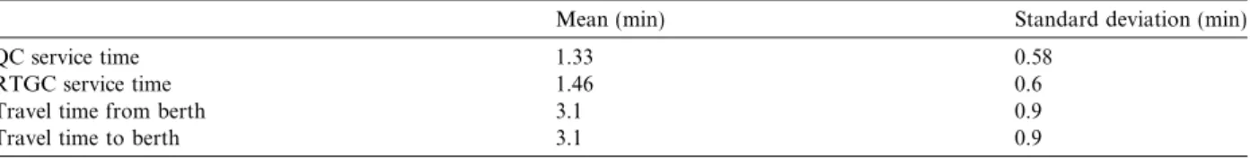
Table 1presents the statistics of the service times at the cranes and the truck travel times at the Port of Balboa. These times are found to fit into normal or log-normal distributions better than exponential distribu-tions. For example, the goodness-of-fit test of QC unloading times is illustrated inFig. 6, where normal and 3-parameter log-normal distributions fit the data quite well.

The value ofsis set to be enough for all trucks in processing and transition to arrive at the queues ahead by the next decision time with 99% statistical signiﬁcance. It should include the processing times at QC or RTGC and the travel times between yard and berth, each of which approximately follow a lognormal distribution. The Fenton–Wilkinson’s method (Hekmat, 2006) is used to approximate a sum of lognormal distributions, and the value ofsis calculated to be 7.65 min.

Table 1

Service time statistics at the Port of Balboa

Mean (min) Standard deviation (min)

QC service time 1.33 0.58

RTGC service time 1.46 0.6

Travel time from berth 3.1 0.9

(10)

3.1. Steady-state analysis with the cyclic queue model

We first use(1)–(7)to calculate the expected time for unloading allD= 230 containers in the steady state, with various equipment combinations. SeeFig. 7. Solutions become feasible for all combinations of QC and RTGC with a minimum of 8 trucks. Also, increasing the number of QC and RTGC from 1 to 2 or 3 does not significantly reduce the operating time when the number of trucks is less than 7. Note that increasing the num-ber of RTGC to 2, while keeping only 1 QC, did not improve the processing rate significantly. This is intuitive since the processing rates of QC and RTGC are similar, and the system can only run as fast as the slower stage. In that case, vehicles will be queued at stage 2 because they are being served at almost twice the rate at stage 4.

System operating costs are then calculated for all combinations of QC, RTGC and trucks that are feasible, as shown inFig. 8. Efficiency enhancement from increasing the number of QC and RTGC are observed only when enough trucks are provided. Out of all combinations it is found that operating 2 QC and 2 RTGC with 15 trucks yields the minimum cost of 87.6 truck-hour cost equivalents. Using only 1 QC and 1 RTGC gener-ates significantly higher costs, given that it is relatively expensive to have the vessel waiting at the deck. Using 3 QC and 3 RTGC does not speed up the operation enough to compensate for the increase of operating costs. These results clearly show the tradeoff between having faster container throughput (while using more resources per unit time) and saving the size of the fleet (while having longer cycles).

3.2. Operational ﬂeet management with MDP

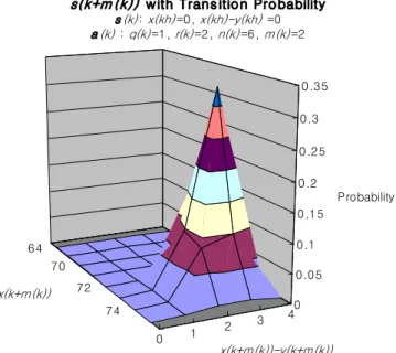
The simulation module and MDP are coded and compiled in the Microsoft Visual C++ Environment, and executed on a personal computer with a 3.0 GHz Pentium 4 CPU and 1.24GB RAM. The MDP is solved within 4 min of CPU time. The transition probabilities are calculated from 500 simulation runs. An example

(11)

of the simulated probabilities is depicted inFig. 9, wherex(k) = 0 andx(k)y(k) = 0 before 1 QC, 2 RTGC, and 6 trucks are operated for two hours (i.e.,m(k) = 2). At the end of the 2-h period, there is a probability of

0 1 2 3 4 5 6 7 8 9 10 11 12 13 14 15 2 3 4 5 6 7 8 9 10 11 12 13 14 15 16 Number of Trucks Hours 1QC + 1RTGC 1QC + 2RTGC 2QC + 2RTGC 2QC + 3RTGC 3QC + 3RTGC

Fig. 7. Expected unloading time in steady-state operations.

40 60 80 100 120 140 160 180 4 6 8 10 12 14 16 Number of Trucks

Cost (Truck Wages * Hour)

1QC + 1RTGC 1QC + 2RTGC 2QC + 2RTGC 2QC + 3RTGC 3QC + 3RTGC

(12)

0.3373 that x(k+m(k)) = 73 containers will be unloaded from the vessel, x(k+m(k))y(k+m(k)) = 3 trucks will be waiting at the yard, and n(k)[x(k+m(k))y(k+m(k))] = 3 trucks will be waiting at the berth.

It is not easy to plot the optimal policy from MDP due to the high dimensions of the state and control variables. Table 2gives the most likely sample-path solution for s= 7.65 min, where the optimal action is to use the samea(k) = [q(k),r(k),n(k),m(k)] = [2, 2, 13, 3] for three consecutive hours to complete the unload-ing task. In this case, the positive value ofsserves as a penalty against ﬂeet size changes. The total cost for this sample path solution is 100.32 truck-hour equivalents.

For comparison, we consider the aggressive case wheresis set to be zero. The most likely sample-path solu-tion is given in Table 3. The optimal action in the ﬁrst hour isa(1) = [2, 2, 12, 1]. Due to the stochasticity,

there are many possible states at the beginning of the second hour. Among them,

s(2) = [x(1),x(1)y(1), 1] = [77, 5, 1] has the largest transition probability of 0.264. J(s(k)) represents the expected ‘‘cost-to-go.” The minimum expected total cost for this most likely sample-path solution is 97.11 truck-hour equivalents, which is only 3.2% lower than the cost withs= 7.65 min.

For additional comparison, the optimal solution from the cyclic queue model, i.e., a fleet configuration of 2 QC, 2 RTGC and 15 trucks, is examined in the MDP framework with log-normal service times (rather than exponential times). Table 4 shows the most likely sample-path solution under this fixed fleet configuration. The time used for unloading all the containers is 3 h and the total cost is 106.48 truck-hour cost equivalents,

Fig. 9. Example of simulated transition probabilities.

Table 2

The most likely sample-path for operational ﬂeet management withs= 7.65 min

Period (k) 1 2 3 4 5 x(kh) – 230 y(kh) – 230 x(kh)y(kh) – 0 Number of truck,n(k) 13 0 Number of RTGC,r(k) 2 0 Number of QC,q(k) 2 0 m(k) 3 1 J(s(k)) 100.32 0 Transition probability 0.986 1

(13)

about 20% larger than the predicted result of 87.58 from the cyclic queue model. Although, by definition, the most likely sample-path cost from MDP is not exactly equivalent to the expected cost from the cyclic queue model, it is obvious that the cost difference partly comes from the assumptions of steady-state operations and exponentially distributed service times. The cost of 106.48 is also higher than 100.32, the cost under the con-servative strategy (s= 7.65). These observations demonstrate that as a complement of the cyclic queue model, which is suitable for long-term fleet planning, the MDP model can further improve system performance by varying fleet configurations in real time.

4. Fleet allocation among multiple berths

In many cases, the terminal has full information on vessels’ arrival and departure schedules atB> 1 berths and needs to determine an allocation plan for theqmax QCs,rmaxRTGCs, and nmaxtrucks. To simplify the

problem, we only allow terminals to change conﬁguration at ﬁxed timeskh,k= 1, 2,. . .,K.

Assume that the number of containers unloaded at berthb by timekh isxb(k), and the number of QCs,

RTGCs, and trucks allocated to berthb isqb(k),rb(k), andnb(k). The allocation is constrained by available

resource: XB b¼1 q_bðkÞ6_q max; XB b¼1 rbðkÞ6rmax; XB b¼1 nbðkÞ6nmax 8k: ð19Þ

Assuming that within each period the cyclic queue model approximately holds and the throughputSis given by(7) as a function ofqb(k),rb(k), andnb(k). Thus the expected increase in unloaded containers is

xbðkþ1Þ ¼xbðkÞ þh=SðqbðkÞ;rbðkÞ;nbðkÞÞ: ð20Þ At berthb, the consecutive vessels have scheduled departure times,kb1h,. . .,kbjh,. . .(assuming that they fall

onto a time lattice of intervalh) and predetermined numbers of containers to unloadDb1,. . .,Dbj,. . .This Table 3

The most likely sample-path for operational ﬂeet management withs= 0

Period (k) 1 2 3 4 5 x(kh) 0 77 154 230 y(kh) 0 72 149 230 x(kh)y(kh) 0 5 5 0 Number of truck,n(k) 12 11 12 0 Number of RTGC,r(k) 2 2 2 0 Number of QC,q(k) 2 2 2 0 m(k) 1 1 1 1 J(s(k)) 97.1074 64.507 32.3738 0 Transition probability 0.264 0.23 0.996 1 Table 4

The most likely sample-path with the cyclic queue model solution

Period (k) 1 2 3 4 5 x(kh) – 230 y(kh) – 230 x(kh)y(kh) – 0 Number of truck,n(k) 15 0 Number of RTGC,r(k) 2 0 Number of QC,q(k) 2 0 m(k) 3 1 J(s(k)) 106.28 0 Transition probability 0.986 1

(14)

translates into a constraint on the operations, such that the cumulative number of containers unloaded to be at least the cumulative number scheduled before the departure of that vessel:

xbðkbjÞP

Xj i¼1

Dbi 8b;j: ð21Þ

When we assume that all vessels’ arrival and departure times are known and ﬁxed, the vessel waiting costs become constant. The ﬂeet management problem is equivalent to minimize the following:

MinX K k¼1 XB b¼1 ½cqqbðkÞ þcrrbðkÞ þctnbðkÞ h;

such that(1)–(7), (19), (20) and (21)are satisﬁed. The solution techniques introduced for a single berth will still be applicable to this multi-berth problem. In case the cyclic queue model is not appropriate to describe the dynamics within intervalh, the simulation results presented in Section2.2can be applied to substitute(20). 5. Conclusions

In this paper we presented modeling frameworks for the planning and management of optimal marine terminal fleets to unload cargos from container vessels. A cyclic queue model was first developed to yield long-term steady-state performances. It assumes exponentially distributed service times in order to obtain closed-form analytical results. A complementary MDP model is then presented to provide real-time operating strategies. The MDP models allow for dynamic fleet allocations and general service time distributions. In prac-tice, the cyclic queue model can help port operators to conduct strategic planning of their fleets, while the MDP model can help improve system performance by allowing for a more efficient use of the equipment in real time. Both models are also suitable for extensions to terminals with multiple berths.

The frameworks (e.g., the MDP models) introduced in this paper can be extended in several directions. For example, fixed costs for changing fleet configuration can be easily incorporated into the cost formula. The sys-tem dynamics Eqs.(8)–(14)can be equivalently written in terms of discrete jump functions and the transition probabilities can be estimated with discrete event simulations. The stochastic effect of crane breakdowns can be considered in the transition probability simulations. More detailed operating requirements, such as han-dling, storage of refrigerated containers and security screening, can be easily incorporated into the modeling framework. It might also be desirable to extend both the cyclic queue model and MDP model to accommodate the double cycling strategy proposed byGoodchild and Daganzo (2006). Finally, the continuous dynamic pro-gramming approach may be applied to optimizing fleet configurations in a non-discrete time horizon. Acknowledgement

The authors thank Mr. Edwin Lewis for providing data of the Port of Balboa, Panama. References

Bish, E.K., Leong, T., Li, C., Ng, J.W.C., Simchi-Levi, D., 2001. Analysis of a new vehicle scheduling and location problem. Naval Research Logistics 48, 363–385.

Chen, Y., Leong, Y.T., Ng, J.W.C., Demir, E.K., Nelson, B.L., Simchi-Levi, D., 1998. Dispatching automated guided vehicles in a mega container terminal. In: Paper presented at the Institute for Operations Research and the Management Sciences (INFORMS) Conference, Montreal, Canada.

Garrido, R.A., Allendes, F., 2002. Modeling the internal transport system in a container port. Transportation Research Record: Journal of the Transportation Research Board 1782, 84–91.

Goodchild, A.V., Daganzo, C.F., 2006. Double-cycling strategies for container ships and their eﬀect on ship loading and unloading operations. Transportation Science 40 (4), 473–483.

Goodchild, A.V., Daganzo, C.F., 2007. Crane double cycling in container ports: planning methods and evaluation. Transportation Research Part B 41, 875–891.

Gordon, W.J., Newell, G.F., 1967. Closed queuing systems with exponential servers. Operations Research 15 (2), 254–265. Hekmat, R., 2006. Ad-hoc Networks: Fundamental Properties and Network Topologies. Springer, Netherlands.

(15)

Kim, K.H., Bae, J.W., 1999. A dispatching method for automated guided vehicles to minimize delays of containership operations. International Journal of Management Science 5 (1), 1–25.

Koenigsberg, E., Lam, R.C., 1976. Cyclic queue models of ﬂeet operations. Operations Research 24 (3), 516–529.

Narasimhan, A., Palekar, U.S., 2002. Analysis and algorithms for the transtainer routing problem in container port operations. Transportation Science 36 (1), 63–78.

Newell, G.F., 1982. Applications of Queuing Theory. Chapman & Hall, New York.

Shields, J.J., 1984. Container stowage: a computer aided preplanning system. Marine Technology 21 (4), 370–382.

Steenken, D., Henning, A., Freigang, S., Voss, S., 1993. Routing of straddle carriers at a container terminal with the special aspect of internal moves. OR Spektrum 15 (3), 167–172.

The World Bank Group, 2006. Port and logistics overview. Washington, DC.<http://www.worldbank.org/transport/ports_ss.htm>. Thomas, B.J., Roach, D.K., 1987. Operating and maintenance features of container handling systems. The World Bank Policy planning

and Research Staﬀ. Infrastructure and Urban Development Department. Washington, DC.

US Army Corps of Engineers, 2004. Consolidated implementation of the New York and New Jersey harbor deepening project-limited reevaluation report.<http://www.nan.usace.army.mil/harbor/lrr/2004/vol3a/economic.pdf>.

Vis, I.F.A., Koster, R., de Roodbergen, K.J., Peeters, L.W.P., 2001. Determination of the number of automated guided vehicles required at a semi-automated container terminal. Journal of the Operational Research Society 52 (4), 409–417.