Short-term hydrological drought forecasting based on different nature-inspired optimization algorithms hybridized with artificial neural networks

Short-Term Hydrological Drought Forecasting

Based on Different Nature-Inspired Optimization

Algorithms Hybridized With Artificial

Neural Networks

NARJES NABIPOUR 1_{, MAJID DEHGHANI} 2_{, AMIR MOSAVI} 3,4,5,6_,

AND SHAHABODDIN SHAMSHIRBAND 7,8

1_{Institute of Research and Development, Duy Tan University, Da Nang 550000, Vietnam}

2_{Technical and Engineering Faculty, Department of Civil Engineering, Vali-e-Asr University of Rafsanjan, Rafsanjan, Iran} 3_{Kalman Kando Faculty of Electrical Engineering, Obuda University, 1034 Budapest, Hungary}

4_{Institute of Structural Mechanics, Bauhaus University Weimar, 99423 Weimar, Germany} 5_{School of the Built Environment, Oxford Brookes University, Oxford OX3 0BP, U.K.} 6_{Department of Mathematics and Informatics, J. Selye University, 94501 Komárno, Slovakia}

7_{Dartment for Management of Science and Technology Development, Ton Duc Thang University, Ho Chi Minh, Vietnam} 8_{Faculty of Information Technology, Ton Duc Thang University, Ho Chi Minh, Vietnam}

Corresponding author: Shahaboddin Shamshirband ([email protected])

This work was supported in part by the Hungarian State and in part by the European Union Project under Grant EFOP-3.6.1-16-2016-00010.

ABSTRACT Hydrological drought forecasting plays a substantial role in water resources management. Hydrological drought highly affects the water allocation and hydropower generation. In this research, short term hydrological drought forecasted based on the hybridized of novel nature-inspired optimiza-tion algorithms and Artificial Neural Networks (ANN). For this purpose, the Standardized Hydrological Drought Index (SHDI) and the Standardized Precipitation Index (SPI) were calculated in one, three, and six aggregated months. Then, three states where proposed for SHDI forecasting, and 36 input-output combinations were extracted based on the cross-correlation analysis. In the next step, newly proposed optimization algorithms, including Grasshopper Optimization Algorithm (GOA), Salp Swarm algorithm (SSA), Biogeography-based optimization (BBO), and Particle Swarm Optimization (PSO) hybridized with the ANN were utilized for SHDI forecasting and the results compared to the conventional ANN. Results indicated that the hybridized model outperformed compared to the conventional ANN. PSO performed better than the other optimization algorithms. The best models forecasted SHDI1 with R2=0.68 and RMSE=

0.58, SHDI3 with R2=0.81 and RMSE=0.45 and SHDI6 with R2=0.82 and RMSE=0.40.

INDEX TERMS Hydrological drought, precipitation, machine learning, hydrology, SPI, PSO, SSA, BBO, GOA.

I. INTRODUCTION

Drought is a natural phenomenon that occurs in all climates. It is a creeping event with an extensive spatial coverage that the determination of the onset and end of drought is diffi-cult [1]. As the drought occurs in every part of the world even-tually, the water resources systems affect by that, and it leads to water shortage in an area during a short to long period. Generally, drought classifies into four types, including mete-orological, hydrological, agricultural and socio-economic

The associate editor coordinating the review of this manuscript and approving it for publication was MalikJahan Khan .

drought [2], [3]. It can be said that drought is a progressive phenomenon that starts with a precipitation deficit as a mete-orological drought. Prolonged metemete-orological drought may lead to hydrological drought resulted in decreasing the dam reservoir volume, river flow, and water level in lakes. Also, a sustained hydrological drought leads to agricultural drought. While drought is considered as a climate variability event, mitigation of its impacts on water resources systems, agri-culture sector, hydropower generation, and associated socio-economic impacts motivated the researchers to establish drought forecasting models. Results of drought forecasting can effectively utilize for water resources decision making,

early warning and applying the drought mitigation strategies. However, due to the complexity of drought phenomenon and its creeping nature, drought forecasting is a challenging issue. In drought monitoring and forecasting, the first and the most essential issue is drought identification and quantifi-cation. For this purpose, from the 1960s, different drought indices were developed based on the individual or multi-ple meteorological or hydrological variables and used for drought monitoring and forecasting. Among all drought indices, standardized precipitation index (SPI) proposed by McKeeet al.[4] (1993) [4] reaches high attention and widely used for drought quantification across the world [5]. Also, several hydrological drought indices were proposed and uti-lized. Surface water supply index (SWSI) [6], standardized runoff index (SRI) [7], and standardized hydrological drought index (SHDI) [5] are the most widely used hydrological drought indices.

After drought quantification, the most crucial issue in drought forecasting is the choice of a suitable model [8]. Physical, conceptual, and data-driven models are widely used for drought forecasting. Physical and conceptual models con-sider the basin processes, so, they are data-intensive and make a complicated model which is appropriate when required data is available [9]. In contrast, data-driven models implement the minimum data without considering the catchment process and act as a black-box model. Data-driven models were used to forecast several meteorological and hydrological variables satisfactorily [10]. In recent years, different types of models including time series [11], [12], neural networks [13]–[18], fuzzy inference systems [19], [20], support vector regres-sion [21]–[23] and copula functions [24]–[26] were utilized for drought forecasting. Most of these researches were car-ried out for meteorological drought forecasting, and few of them were conducted to forecast the hydrological drought indices [27]–[31]. Due to the complexity and non-linear process of drought, using soft computing methods reaches high attention in drought forecasting. Among all machine learning methods, ANN is one of the oldest and maybe the most well-known method. Parallel processing, ability to work with incomplete information, working with noisy data and its ability to learn the patterns are the main factors that make it popular in water resources modeling. In contrast, the same as other models, ANN has several shortcomings. The main disadvantage of ANN is that it is a black-box model, and the intermediate processes between input-output combina-tions were not considered. Besides, the architecture of the ANN is not constant, and the best results in each problem achieve using different architecture, which determines via a trial and error procedure. Also, based on every architecture, appropriate values must be assigned to several parameters, including the weights and biases. So, training the ANN is time-consuming, and it may trap in local minima, which the results are not reliable in this case. To remedy this problem, several optimization algorithms were proposed during the past decades. Recently a new category of optimization algo-rithms so-called nature-inspired was developed. Based on the

FIGURE 1. Location of the Dez dam and the precipitation stations in Iran (after Dehghani et al. 2019a).

authors’ knowledge, there is no study that evaluated the cou-pled of intelligent models with nature-inspired optimization algorithms for hydrological drought forecasting. Threfore, in this study, the ANN coupled with four optimization algo-rithms to forecast the hydrological drought. For this purpose, the Dez basin in the southwestern of Iran was considered as the case study. Dez dam is one of the highest dams in Iran that its reservoir is used for hydropower generation and irrigation of the farming lands in the downstream of the dam. Therefore, hydrological drought in this basin can affect agricultural pro-duction and reducing hydropower generation. The SHDI was calculated based on the inflow to the dam. Then, ANN was coupled by SSA, BBO, GOA and PSO algorithms to forecast the hydrological drought. The SSA, BBO, GOA and PSO algorithms have recently shown promising results in optimiz-ing machine learnoptimiz-ing models for hydrological applications [30]. Thus, they have been confidently selected for this study. The rest of the paper is organized as follows. Section II contains the case study, SPI, and SHDI calculation, selec-tion of input-output combinaselec-tions, ANN and optimizaselec-tion algorithms. In section III, the results were presented and a detailed comparison between different models was carried out. Finally, a brief description of the findings of this research was drawn as the conclusion in section IV.

II. MATERIAL AND METHODS A. CASE STUDY

The Dez Dam is a double curvature arch dam in south-western Iran constructed and operated in 1963 (Figure 1). It is located on the Dez River, which is one of the longest rivers in Iran (510 km). The reservoir volume and the dam height are 3340×106m3and 203mrespectively [32]. It is a multi-objective dam that is designed and constructed for hydropower generation, Irrigation, flood control, and water supply. About 125000 ha of the agricultural area downstream, the Dez dam is irrigated by water released from the dam. Also, 520 MW electricity is generated by hydropower plants installed downstream of the dam.

The dam inflow is measured at Tele-Zang station located just upstream of the dam. There are four meteorological sta-tions in the Dez catchment and ten stasta-tions around the catch-ment (Figure 1). The hydrometric and precipitation data were gathered from Iran’s Water Resources Management Com-pany (http://www.wrm.ir/index.php?l=EN) and Iran Meteo-rological Organization (http://www.irimo.ir/eng/index.php). The monthly data covered the range of October 1963 to September 2017.

The average precipitation over the basin was interpolated using the inverse distance weight (IDW) method.

B. SPI AND SHDI CALCULATIONS

Several meteorological drought indices were proposed by researchers during the past decades, among all, SPI received high attention, and it is widely used for drought moni-toring and forecasting in different countries [26]. As SPI is calculated based on just precipitation, it is a simple drought index, and due to the normality, it is possible to use it in spatial and temporal comparison. For SPI calcula-tion, first, a proper probability distribution function (default function is gamma) is fitted to a long-term data (at least 30 years). g(x)= 1 βα_{0 (α)}xα−1e −x β _{for x} >0, α, β >0 0 (α) = Z ∞ 0 yα−1e−ydy (1)

where0 (α)is the gamma function andαandβare the shape and scale parameters respectively [26].

Then its cumulative probability distribution will transform via an equal probability transformation to the normal dis-tribution with mean zero and standard deviation of unity. The transformed values are SPI. This procedure can be done for every time scale. Positive and negative values of SPI show greater and less than median precipitation, respectively. Dehghani et al. [5] developed the SHDI by replacing the precipitation with discharge.

TABLE 1. SPI and SHDI classification (Dehghani et al., 2017).

Table 1 shows the classification of SPI and SHDI. The pro-cedure of SPI and SHDI calculation was presented elsewhere and one may refer to [33]–[38].

C. DROUGHT FORECASTING SCENARIOS AND INPUT-OUTPUT COMBINATIONS

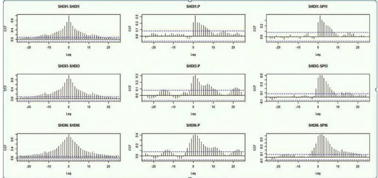
Drought events happen in the short term and long-term peri-ods. Typically, drought is considered long term if it sustained more than six months. As dam operation and water allo-cation to different sectors, including agricultural, domestic, or industrial need short term information about drought/wet condition, in this research, hydrological drought for 1, 3, and 6 months ahead were forecasted. So, the SHDI was calculated for 1, 3, and 6 months’ time scale, which hereafter is called SHDI1, SHDI3 and SHDI6. These three time scales were considered as the states that must be forecasted. In the next step, it is needed to determine the best predictors for these three states. As it is evident, the hydrological drought in previous months may be a suitable predictor. Also, the pre-cipitation and meteorological drought in previous months can be considered as appropriate predictors. So, to prepare a set of predictors for hydrological forecasting, cross-correlation analysis was carried out. Results are presented in Figure 2. Based on this figure, SHDI in all time scales has the highest cross-correlation with its lags and in the next steps with SPI and precipitation. So, these parameters could be used as the predictors for SHDI forecasting. On the other hand, to evaluate the capability of hybrid models in forecasting SHDI in several ahead months, for SHDI1 and SHDI3, three input combinations were considered. Also, six input combi-nations were considered for SHDI6. Therefore, three states and 12 input combinations resulted in 36 input-output com-binations for modeling, as presented in Table 2.

D. ARTIFICIAL NEURAL NETWORKS

Artificial neural networks were first introduced in 1943 by Pitts and McCulloch (ASCE, 2000). In the mid-1980s, Mc Clelland and Rumelhart developed backpropagation algorithms that could be used to train complex net-works. Since the early 1990s, these models have also been used successfully in hydrology, including modeling of rainfall-runoff processes, river flow prediction, and so on. Dehghani and Moradkhani [25] outlined the benefits of the ANN model, which has made widespread use in various fields:

- Having the characteristic of distributed information pro-cessing.

- Ability to detect the relationship between input and output variables without physical consideration of the phenomenon. - Proper performance of these models even with measure-ment error.

The way neural networks work is inspired by the way neural neurons work. In neurons, information is received by dendrites, reaching the body of the cell (including the nucleus and other protective components), stimulating the cell, providing the body with the energy needed for neu-ron activity, and it operates on the input signals, which is modeled by a simple operation and compared to a thresh-old level. Then the result is transferred to the next cell by

FIGURE 2. Cross-correlation analysis between SHDI, SPI, and precipitation.

the axons. An artificial neural network does just that. A detailed

explanation of ANN presented elsewhere (ASCE, 2000, Dehghaniet al.[26], [5], [31]). Mosaviet al.[30] reviewed the state of the art applications of ANN in hydrological models along with a comparison with other machine learning models. After selecting the inputs, it is time to build a neural network model to predict drought. A MLP network with backpropagation training algorithm was considered in this research. The main challenging issue in ANN modeling is assigning the appropriate weights and biases, which are determined during the iteration process. To remedy this problem, it is possible to use optimization algorithms, which are powerful tools in this field which are discussed in the next sections.

E. PARTICLE SWARM OPTIMIZATION

The particle swarm optimization is a meta-heuristic algorithm proposed by Eberhart and Kennedy [39] for global optimiza-tion. It is inspired by the animal swarming such as birds and fish. In the PSO, there are several particles distributed in the N-dimensional search space. Each particle has its random velocity and position. Particles move to the location of the best fitness, which is obtained by them and the best position of the neighbors’ particles (local and global bests) [40]. Com-bination of the information of the current location for each particle and the best position it has been in, as well as the information of one or more particles with the best location, leads to movement. After the mass movement, one step of the algorithm ends. These steps are repeated several times until the desired result is obtained. The flowchart of the PSO algorithm was drawn in Figure 3. Also, for more information about the PSO, one may refer to [39], [41]. The novel machine learning models using PSO have been recently emerging. PSO have been shown to improve the performance of various hybrid machine learning methods through tuning the model parameters in hydrological applications [30].

F. BIOGEOGRAPHY-BASED OPTIMIZATION

ABBO was developed based on the biogeography concept by Simon (2008) [42]. Simply, the algorithm works as follows. There are some isolated islands so-called the habitat. Differ-ent spices live in these islands. Each island has a habitat suit-ability index (HSI), which means that some islands are more appropriate for habitation. HSI is related to some features such as temperature, rainfall, topography, etc., which called suitability index variables (SIVs). BBO shows how species migrate. Habitats with high HSI have several creatures, while low HSI associated with few creatures. So, a high HSI habi-tats tend to migrate to other habihabi-tats. This transferring called emigration and the process called immigration. Therefore, high HSI has a high emigration rate while low HSI has high immigration rate [43]. The BBO algorithm is based on migration and mutation. In BBO, a vector of real numbers which are SIV considered as a solution [44]. The fitness function is calculated using the objective function. It must be

FIGURE 3.Flowcharts of PSO, BBO, SSA and GOA optimization algorithms.

noted that the solutions with high and low HSI are considered as good and bad solutions, respectively. The probabilistic approach is used to share the information between habitats. The modification of each solution is based on the emigration and immigration rates. The elitism process is governed in the BBO algorithm, and just a number of best solutions are transferred to the next iteration [43]. As each solution has its own probability, the one with low probability has the chance to mutate while the solution with high probability has little chance to mutate. BBO has shown promising results when using in a hybrid form with machine learning methods to tune the model parameters [30]. Detailed description of the BBO presented elsewhere [42]–[44], and the flowchart of BBO is shown in Figure 3.

G. SALP SWARM OPTIMIZATION

SSA is a recent novel nature-inspired meta-heuristic opti-mization algorithm proposed by Mirjaliliet al.[45]. Salps live in the deep ocean often form a swarm so-called salp chain. This chain helps them to obtain more kinetic energy during the pursuing of the food source. SSA mitigates the inertia to the local optima, but it is not possible to find the global optimum in some cases, and this is one of the limitations of this algorithm. Salps classify into two groups, the leader, the one in the head of the chain and the followers. The leader

guides the direction, and the followers follow each other. The position of salps is defined in an N-dimensional search space. N is the number of variables in the problem. F is defined as the food source in the search space. So, the position of the leader is determined by:

x_j1= ( Fj+_{c1 ubj}−_lbj c2+lbj c3≥0.5 Fj−c1 ubj−lbjc2+lbj c3<0.5 ) (2) wherex_j1is the position of the leader,Fj is the position of

food source in the jth dimension, ubj andlbj are the upper

and lower limits of jth dimension andc1,c2andc3are random

values.c1is calculated based on the equation (3) whilec2and

c3generated randomly inside [0,1].

c1=2e − 4t

Tmax()

2

(3) where, t and Tmax are the current and maximum number

of iterations, respectively. The flowchart of SSA is shown in Figure 3.

H. GRASSHOPPER OPTIMIZATION ALGORITHM

The GOA is a meta-heuristic algorithm proposed by Mirjalili et al. [46]. GOA is a population-based method mimicking the behavior of grasshopper swarms and their social interaction. Although the grasshoppers are individual in nature, they join in huge swarm. Food source seeking is one of the most essential characteristics of the swarming of grasshoppers by dividing the search process into exploration and exploitation. The position of each grasshopper in the swarm is based on the social interaction between it and the other grasshoppersSi, the gravity force on itGiand the wind advectionAias presented in equation (4):

Xi =Si+Gi+Ai Si = XN j=1 j6=i s dij _ˆ dijdˆij= xj−xi dij s(r)=fe −r l −e−rdij =xj−xi (4)

where,dijis the distance between i-th and j-th grasshopper,

s is the strength of social forces, f is the intensity attrac-tion, andl is the attractive length scale. When the distance between two grasshoppers is in the interval [0,2.079], then the repulsion force happens, the distance equal 2.079 leads to neither attraction nor repulsion and the distance greater than 2.079 causes an increase in attraction force, then it decreases gradually when it reaches to 4.

The gravity force calculated as follows:

Gi= −gegˆ (5)

where, g is the gravitational constant, andegˆ is a unity vector toward the center of the earth.

Wind advection is described as follows:

Ai =uewˆ (6)

where, u is a constant drift, and eˆw is a unit vector in the

direction of wind (Mirjalili et al. [46], 2018). A detailed

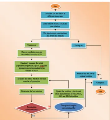
FIGURE 4. The proposed framework for optimizing the ANN using PSO, BBO, SSA and GOA algorithms for hydrological drought forecasting.

explanation about this newly developed algorithm was pre-sented in [46] and the flowchart of GOA is shown in Figure 3 Based on Figure 4, the proposed hybrid model works as follows:

Step 1. Calculate SPI and SHDI in different time scales. Step 2. Consider an input-output combination based on Table 3.

Step 3. Prepare the input and output based on step 2. Step 4. Create the initial ANN architecture.

Step 5. To couple each of the optimization algorithms with ANN, Create the initial population of particles, determine the initial location (for PSO and GOA), velocity (for PSO), emigration and immigration rate (for BBO), set initial bound limits (for SSA) and objective functions.

Step 6. Evaluate the objective function based on the root mean squared error (RMSE) for each particle and determine the best solution.

Step 7. Update the location, velocity, emigration and immi-gration rate and evaluate the fitness function.

Step 8. If the stopping criterion was met, then the algorithm terminated, and the weights were considered as the best val-ues for ANN. Else, all the parameters are updated based on step 7.

I. EVALUATION CRITERIA

To evaluate the capability of different algorithms used for optimizing the ANN in hydrological drought forecasting, several statistical and graphical tests were used. Among all statistical indices, coefficient of determination (R2), relative absolute error (RAE), mean absolute error (MAE), root mean squared error (RMSE), index of agreement (d), confidence

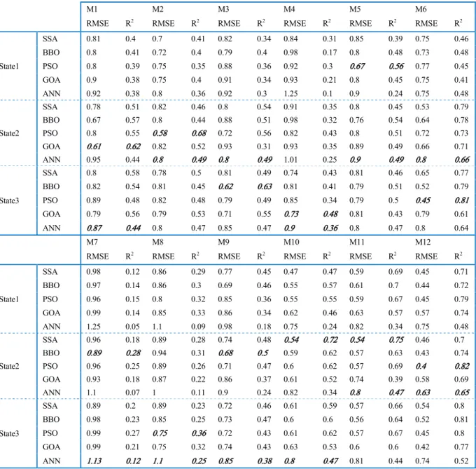
TABLE 3. Results of ANN and hybrid models in the test stage.

index (CI) and Nash–Sutcliffe coefficient (NSE) are used. A detailed description of these indices was presented by Dehghaniet al.[5]. Also, scatter plot, box plot of prediction and observations and errors and error distribution are used to evaluate the performance of each algorithm in hydrological drought forecasting. Also, RDR index which proposed by Memarzadehet al.[47] was utilized for model performance evaluation. RDR=Sign(Estimated Kx −Measured Kx) log Estimated Kx Measured Kx

Also, Wilcoxon and Freidman tests were utilized to evaluate the equality of mean in the observed and forecasted time series.

III. RESULTS

In this section, the performance of customary ANN and the hybrid of ANN with SSA, BBO, PSO, and GOA optimization algorithms were discussed.

A. SPI AND SHDI CALCULATION

After conducting the non-parametric tests on the data to evaluate the quality of data and filling the gaps, the average of precipitation was estimated using the Kriging method. Then, several probability distribution functions were fitted to the precipitation and discharge time series. Gamma and Log-normal functions were selected as the best fit for SPI and SHDI, respectively. In the next step, 36 input-output combinations were prepared for modeling.

B. COMPARISON OF NEW HYBRIDIZED MODELS WITH THE CONVENTIONAL ANN

The quantitative results of hybridized models and conven-tional ANN are presented in Table 3. Also, the best results for M1 to M12 were bolded in the table. The results could be compared in several aspects. Based on the states, just one of the best-hybridized models lies in state 1, while 7 and 4 best models lay in state 2 and state 3, respectively. For conventional ANN, 5 and 7 best models were laid in state 2 and state 3, respectively. It shows that state 1 is not suitable for modeling. It means that although the SHDI has a strong correlation with its previous lags, it is not only a function of its previous values. Other factors such as pre-cipitation or meteorological drought, which happens before hydrological drought joint with SHDI in previous lags, can improve the results considerably. Also, precipitation jointed with SHDI values in previous months are better predictors for SHDI forecasting than SPI jointed with SHDI, especially in hybridized models. A precise evaluation shows that for M1 to M3, the best models are mostly in state 2. It means that to forecast the hydrological drought in a monthly time scale, which represents as SHDI1, precipitation, and SHDI in previous months are the best inputs. For M4 to M6, two of the best models are in state 3, and one of them is in state 1. So, it is possible to say that for SHDI3 forecasting, state 3, which contains SPI and SHDI in previous steps as input, is the best. For M7 to M12, five of the best models are in state 2, which shows the same as M1 to M3, precipitation, and SHDI in previous months are the best inputs.

Results of Table 3 indicate that hybridized models are supe-rior to the conventional ANN in all states and M1 to M12. The RMSE and R2 were improved between 0.1 and 0.2 in almost all input-output combinations. It means that the hybridizing ANN with nature-inspired optimization algorithms strongly enhances the results.

Based on Table 3, it is possible to compare the optimization algorithm for hydrological drought forecasting. SSA, BBO, PSO, and GOA algorithms hybridizing with ANN produced the best results in 2, 3, 5, and 2 cases for M1 to M12, respectively. According to this fact, PSO is superior to others. SSA performed as the best algorithm in M10 and M11, BBO produced the best results in M3, M7 and M9, PSO in M2, M5, M6, M8 and M12 and GOA in M1 and M4. So, SSA is the best for SHDI6 forecasting while BBO for SHDI1 and SHDI6, GOA for SHDI1 and SHDI3 and PSO for all of them. Again it can be concluded that PSO is the best algorithm to hybridize with ANN for hydrological drought forecasting.

Finally, it is possible to evaluate the input combinations in hydrological drought forecasting. Based on Table 3, M1 to M3 were used to forecast SHDI1 while M4 to M6 and M7 to M12 were used to forecast SHDI3 and SHDI6, respectively. Based on the results in Table 3, M2 in state 2 performed as the best model to forecast SHDI1. It shows that the precipitation and SHDI in the previous one and two months are the best predictors for SHDI1 forecasting. M6 in state 3 shows the best

TABLE 4.Results of Friedman and Wilcoxon tests.

performance for SHDI3 forecasting. So, the SPI and SHDI values in the previous three months are the best predictor for SHDI3 forecasting. However, it is worthy to note that the results of M4 in state 3 are more valuable than the results of M6 in some aspects.

First, the model needs two predictors while in M6, the model needs six predictors. Also, in M4, the SPI and SHDI values of three months ago are the predictors, which it means that the model forecast SHDI for one season ahead. However, M6 uses the SHDI3 values in the last month as the predictor, which means that generally, 2/3 of the information that must be forecasted is available in predictors. Based on these facts, M6 results are more precise, while M4 results are more valuable. This is the fact that it is true for M7 to M12. M12 in state 3 is the most accurate model, while the results of M7 are more valuable.

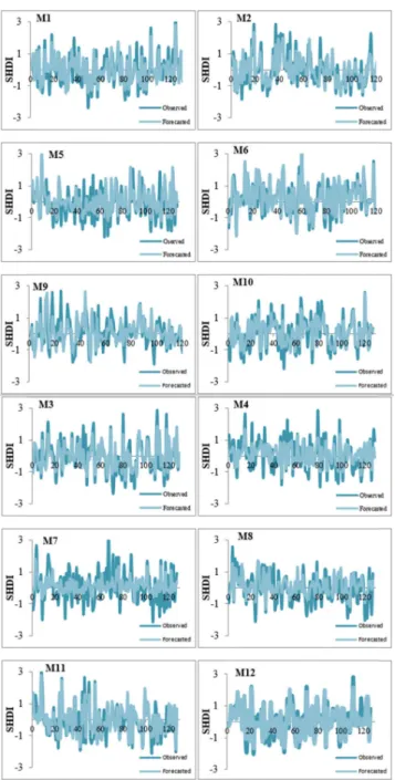
The observed and forecasted time series in the test stage were plotted in Figure 5. According to Figure 5, in M1 to M12, the models are capable of recognizing the pattern, and the observed and forecasted time series changes with the same pattern. However, none of the models are capable of forecasting the exact extreme values. Among all, M1, M11 and M12 had the best performance, and the observed and predicted values are in general agreement even in extreme values.

While the statistical indices are promising and the plots of observed and forecasted time series showed a general agreement between the observed and forecasted SHDI values, however, it is needed to examine the results with statistical tests to ensure the robustness of the modeling. For this pur-pose, Wilcoxon test and Friedman test were utilized. Results were presented in Table 4.

Based on the results of Table 4, except M5 model, the null hypothesis (µ1 = µ2) was accepted at least in one of the

test which means that the mean of observed and forecasted values have no meaningful difference. However, the null hypothesis was rejected in both tests for M5, which shows the meaningful difference in the mean of observed and forecasted time series. So, although M5 has acceptable R2 and RMSE, but there is a significant difference between the mean of observed and forecasted SHDI values reproduced using M5 model. So, besides the statistical indices such as R2 and RMSE, it is necessary to examine the results using statistical tests.

FIGURE 5. Time series of observed and forecasted SHDI using the hybridized models in the test stage.

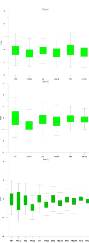
The box plot of observed and forecasted values using ANN and hybrid models were plotted in Figure 6. In the state 1, all hybrid models performed better than ANN, especially in wet conditions (SHDI>1).

The mean in hybrid models is the same as the mean of observations, and the positive values of SHDI were repro-duced almost the same as observed values. However, none of the hybrid models were capable of reproducing drought conditions appropriately.

Generally, M2 performed better in state 1. Also, in state 2, the hybrid models performed better than conventional ANN. Among all, M6 is capable of reproducing both negative and positive values of SHDI while M4 and M5 could not

FIGURE 6. Box plot of observed and forecasted SHDI using the hybridized models in the test stage.

reproduce the extreme values. In the state 3, also, the hybrid models performed far better than ANN. None of the mod-els reproduce the extreme drought condition, but M11 and M12 were superior. In the next step, the boxplot of error for all models was plotted and presented in Figure 7. In the state 1, M2 has the least error while in state 2 and state 3, M6 and ANN6 and M12 have the least error, respectively.

FIGURE 7. Box plot of error in forecasting SHDI using the hybridized models in the test stage.

The RDR was calculated and plotted in Figure 8. Based on Figure 9, the error normally distributed in M1 to M3, which shows that generally, the models overestimation and underestimation are somehow the same. In the state 1, M2 has the least normalized error, which shows the superiority of the model. Also, in state 2, M6 is superior, while the error normally distributed in M4 to M6. In the state 3, the least

FIGURE 8. Standardized normal distribution graph of the RDR values for the SHDI forecasting in the test phase.

error assigned to M9, M8, and M7, respectively. However, M9 has underestimation while M8 and M7 have overes-timation. In the next step, M11 and M12 have the least error, respectively, and the error normally distributed, which resulted in similar overestimation and underestimation.

The empirical cumulative distribution function for M1 to M12 was plotted in Figure 9. In the state 1, all three models performed nearly the same, while M2 has the least error. State 2 and 3 show that M6 and M12 reproduce the SHDI3 and SHDI6 with the least error, respectively. It means that with a given threshold error level, the performance of M6 and M12 is higher than the other models.

Finally, the number of class changes in the forecasting time series compared to the observed values calculated and tabulated in Table 5. For state 1, the models forecasted the correct class in more than 76%. Among all, M2 was the best, which forecasted the accurate classes in 82%, and 17% of

TABLE 5. Number of exact forecast and class change in test stage using hybridized models.

FIGURE 9. The threshold statistic of selected models.

forecasted SHDI1 have one class change compared to the observed data. In the state 2, M6 is superior with 74% of exact forecasting, while for state 3, M12 with 79% of exact

forecasting performed better than other models. Based on the different statistical and graphical analysis, it can be concluded that among all models, M2, M6 and M12 are superior in state 1, state 2 and state 3, respectively.

IV. CONCLUSION

In this research, short term hydrological drought was fore-casted using conventional ANN and hybridized of ANN with nature-inspired optimization algorithms. For this purpose, SSA, BBO, PSO and GOA algorithms were utilized. To fore-cast the hydrological drought, SHDI was calculated in 1, 3 and 6 months time scales. Precipitation, SHDI and SPI values in the previous months were used as the predictors based on cross-correlation analysis. Results indicated that the hybridized models are far superior to the conventional ANN, and these models are capable of forecasting the hydrological drought in different time scales. Based on the results, SHDI values in the previous month(s) are not suitable inputs for hydrological drought forecasting, and other parameters such as SPI and especially the precipitation in the previous months can improve the results of forecasting considerably. Also, among all optimization algorithms, PSO outperformed in hybridizing with ANN, and the ANN-PSO was capable of forecasting SHDI in all time scales. It is worthy to note that for SHDI6, it is impossible to accurately forecast the SHDI using M7, M8, M9 and M10. It means that the hydrological drought in this basin varies in short time, and the information of SHDI in the last two months plays a substantial role in SHDI6 forecasting. For future research, the hybrid models of other machine learning methods with nature-inspired opti-mization algorithms are particularly encouraged.

REFERENCES

[1] Z. Hao, F. Hao, V. P. Singh, A. Y. Sun, and Y. Xia, ‘‘Probabilistic prediction of hydrologic drought using a conditional probability approach based on the meta-Gaussian model,’’J. Hydrol., vol. 542, pp. 772–780, Nov. 2016. [2] D. A. Wilhite and M. H. Glantz, ‘‘Understanding: The drought phe-nomenon: The role of definitions,’’Water Int., vol. 10, no. 3, pp. 111–120, 1985.

[3] R. R. Heim, Jr., ‘‘A review of twentieth-century drought indices used in the United States,’’ Bull. Amer. Meteorolog. Soc., vol. 83, no. 8, pp. 1149–1166, 2002.

[4] T. B. McKee, N. J. Doesken, and J. Kleist, ‘‘The relationship of drought frequency and duration to time scales,’’ inProc. 8th Conf. Appl. Climatol., Anaheim, CA, USA, Jan. 1993.

[5] M. Dehghani, B. Saghafian, F. N. Saleh, A. Farokhnia, and R. Noori, ‘‘Uncertainty analysis of streamflow drought forecast using artificial neu-ral networks and Monte-Carlo simulation,’’Int. J. Climatol., vol. 34, no. 4, pp. 1169–1180, Mar. 2014.

[6] B. A. Shafer and L. E. Dezman, ‘‘Development of a surface water supply index (SWSI) to assess the severity of drought conditions in snowpack runoff areas,’’ inProc. 50th Annu. Western Snow Conf., 1982.

[7] S. Shukla and A. W. Wood, ‘‘Use of a standardized runoff index for characterizing hydrologic drought,’’Geophys. Res. Lett., vol. 35, no. 2, 2008, Art. no. L02405.

[8] R. Zhang, Z.-Y. Chen, L.-J. Xu, and C.-Q. Ou, ‘‘Meteorological drought forecasting based on a statistical model with machine learning techniques in Shaanxi province, China,’’Sci. Total Environ., vol. 665, pp. 338–346, May 2019.

[9] A. Belayneh, J. Adamowski, B. Khalil, and B. Ozga-Zielinski, ‘‘Long-term SPI drought forecasting in the Awash River Basin in Ethiopia using wavelet neural network and wavelet support vector regression models,’’J. Hydrol., vol. 508, pp. 418–429, Jan. 2014.

[10] J. F. Adamowski, ‘‘Development of a short-term river flood forecasting method for snowmelt driven floods based on wavelet and cross-wavelet analysis,’’J. Hydrol., vol. 353, nos. 3–4, pp. 247–266, May 2008. [11] D. Ö. Faruk, ‘‘A hybrid neural network and ARIMA model for water

quality time series prediction,’’Eng. Appl. Artif. Intell., vol. 23, no. 4, pp. 586–594, Jun. 2010.

[12] P. Han, P. X. Wang, S. Y. Zhang, and D. H. Zhu, ‘‘Drought forecasting based on the remote sensing data using ARIMA models,’’Math. Comput. Model., vol. 51, nos. 11–12, pp. 1398–1403, Jun. 2010.

[13] A. Mishra and V. Desai, ‘‘Drought forecasting using feed-forward recur-sive neural network,’’Ecolog. Model., vol. 198, nos. 1–2, pp. 127–138, Sep. 2006.

[14] J. F. Santos, M. M. Portela, and I. Pulido-Calvo, ‘‘Spring drought predic-tion based on winter NAO and global SST in Portugal,’’Hydrol. Process., vol. 28, no. 3, pp. 1009–1024, Jan. 2014.

[15] M. H. Le, G. C. Perez, D. Solomatine, and L. B. Nguyen, ‘‘Meteorolog-ical drought forecasting based on climate signals using artificial neural network—A case study in Khanhhoa province Vietnam,’’Procedia Eng., vol. 154, pp. 1169–1175, 2016.

[16] A. Belayneh, J. Adamowski, B. Khalil, and J. Quilty, ‘‘Coupling machine learning methods with wavelet transforms and the bootstrap and boosting ensemble approaches for drought prediction,’’Atmos. Res., vols. 172–173, pp. 37–47, May 2016.

[17] Z. Ali, I. Hussain, M. Faisal, H. M. Nazir, T. Hussain, M. Y. Shad, A. M. Shoukry, and S. H. Gani, ‘‘Forecasting drought using multilayer perceptron artificial neural network model,’’Adv. Meteorol., vol. 2017, May 2017, Art. no. 5681308.

[18] S. Mouatadid, N. Raj, R. C. Deo, and J. F. Adamowski, ‘‘Input selection and data-driven model performance optimization to predict the standardized precipitation and evaporation index in a drought-prone region,’’Atmos. Res., vol. 212, pp. 130–149, Nov. 2018.

[19] M. Ali, R. C. Deo, N. J. Downs, and T. Maraseni, ‘‘An ensemble-ANFIS based uncertainty assessment model for forecasting multi-scalar standard-ized precipitation index,’’Atmos. Res., vol. 207, pp. 155–180, Jul. 2018. [20] M. Ali, R. C. Deo, N. J. Downs, and T. Maraseni, ‘‘Multi-stage

com-mittee based extreme learning machine model incorporating the influence of climate parameters and seasonality on drought forecasting,’’Comput. Electron. Agricult., vol. 152, pp. 149–165, Sep. 2018.

[21] P. Ganguli and M. J. Reddy, ‘‘Ensemble prediction of regional droughts using climate inputs and the SVM-copula approach,’’Hydrol. Process., vol. 28, no. 19, pp. 4989–5009, Sep. 2014.

[22] R. C. Deo, O. Kisi, and V. P. Singh, ‘‘Drought forecasting in eastern Australia using multivariate adaptive regression spline, least square support vector machine and M5Tree model,’’Atmos. Res., vol. 184, pp. 149–175, Feb. 2017.

[23] L. Xu, N. Chen, X. Zhang, and Z. Chen, ‘‘An evaluation of statistical, NMME and hybrid models for drought prediction in China,’’J. Hydrol., vol. 566, pp. 235–249, Nov. 2018.

[24] Z. Liu, T. Törnros, and L. Menzel, ‘‘A probabilistic prediction network for hydrological drought identification and environmental flow assessment,’’

Water Resour. Res., vol. 52, no. 8, pp. 6243–6262, Aug. 2016.

[25] S. Khajehei and H. Moradkhani, ‘‘Towards an improved ensemble pre-cipitation forecast: A probabilistic post-processing approach,’’J. Hydrol., vol. 546, pp. 476–489, Mar. 2017.

[26] M. Dehghani, B. Saghafian, and M. Zargar, ‘‘Probabilistic hydrological drought index forecasting based on meteorological drought index using Archimedean copulas,’’Hydrol. Res., vol. 50, no. 5, pp. 1230–1250, Oct. 2019.

[27] P. Cutore, G. Di Mauro, and A. Cancelliere, ‘‘Forecasting palmer index using neural networks and climatic indexes,’’J. Hydrol. Eng., vol. 14, no. 6, pp. 588–595, Jun. 2009.

[28] T. Sharma and U. Panu, ‘‘Prediction of hydrological drought durations based on Markov chains: Case of the Canadian prairies,’’Hydrolog. Sci. J., vol. 57, no. 4, pp. 705–722, May 2012.

[29] O. Bazrafshan, A. Salajegheh, J. Bazrafshan, M. Mahdavi, and A. F. Maraj, ‘‘Hydrological drought forecasting using ARIMA models (case study: Karkheh basin),’’Ecopersia, vol. 3, no. 3, pp. 1099–1117, 2015. [30] A. Mosavi, P. Ozturk, and K.-W. Chau, ‘‘Flood prediction using machine

learning models: Literature review,’’ Water, vol. 10, no. 11, p. 1536, Oct. 2018.

[31] M. Dehghani, B. Saghafian, F. Rivaz, and A. Khodadadi, ‘‘Evaluation of dynamic regression and artificial neural networks models for real-time hydrological drought forecasting,’’Arabian J. Geosci., vol. 10, no. 12, p. 266, Jun. 2017.

[32] M. Dehghani, H. Riahi-Madvar, F. Hooshyaripor, A. Mosavi, S. Shamshirband, E. Zavadskas, and K.-W. Chau, ‘‘Prediction of hydropower generation using grey wolf optimization adaptive neuro-fuzzy inference system,’’Energies, vol. 12, no. 2, p. 289, Jan. 2019.

[33] D. C. Edwards and T. B. McKee, ‘‘Characteristics of 20th century drought in the United States at multiple scales,’’ Defense Tech. Inf. Center, Fort Belvoir, VA, USA, Atmos. Sci. Paper 634, May 1997, pp. 1–30. [34] M. J. Hayes, M. D. Svoboda, D. A. Wiihite, and O. V. Vanyarkho,

‘‘Moni-toring the 1996 drought using the standardized precipitation index,’’Bull. Amer. Meteorolog. Soc., vol. 80, no. 3, pp. 429–438, 1999.

[35] X. Lana, C. Serra, and A. Burgueño, ‘‘Patterns of monthly rainfall shortage and excess in terms of the standardized precipitation index for catalonia (NE Spain),’’Int. J. Climatol., vol. 21, no. 13, pp. 1669–1691, 2001. [36] B. Lloyd-Hughes and M. A. Saunders, ‘‘A drought climatology for

Europe,’’Int. J. Climatol., vol. 22, no. 13, pp. 1571–1592, Nov. 2002. [37] H. Wu, M. J. Hayes, D. A. Wilhite, and M. D. Svoboda, ‘‘The effect

of data length on the standardized precipitation index calculation,’’Int. J. Climatol., vol. 25, no. 4, pp. 505–520, 2005.

[38] H. Wu, M. D. Svoboda, M. J. Hayes, D. A. Wilhite, and F. Wen, ‘‘Appro-priate application of the standardized precipitation index in arid locations and dry seasons,’’Int. J. Climatol., vol. 27, no. 1, pp. 65–79, Jan. 2007. [39] R. Eberhart and J. Kennedy, ‘‘A new optimizer using particle swarm

theory,’’ inProc. 6th Int. Symp. Micro Mach. Human Sci., Nov. 2002, pp. 39–43.

[40] R. C. Eberhart. P. K. Simpson, and P. K. Dobbins,Computational Intelli-gence PC Tools. Boston, MA, USA: Academic, 1996.

[41] Y. Liu, Y. Bai, Z. Xia, and J. Hou, ‘‘Parameter optimization of Depressurization–to–Hot–Water–Flooding in heterogeneous hydrate bear-ing layers based on the particle swarm optimization algorithm,’’J. Natural Gas Sci. Eng., vol. 53, pp. 403–415, May 2018.

[42] D. Simon, ‘‘Biogeography-based optimization,’’IEEE Trans. Evol. Com-put., vol. 12, no. 6, pp. 702–713, Dec. 2008.

[43] A. Nazari and A. Hadidi, ‘‘Biogeography based optimization algorithm for economic load dispatch of power system,’’Amer. J. Adv. Sci. Res., vol. 1, no. 3, pp. 99–105, 2012.

[44] K. T. Chaturvedi, M. Pandit, and L. Srivastava, ‘‘Self-organizing hier-archical particle swarm optimization for nonconvex economic dis-patch,’’ IEEE Trans. Power Syst., vol. 23, no. 3, pp. 1079–1087, Aug. 2008.

[45] S. Mirjalili, A. H. Gandomi, S. Z. Mirjalili, S. Saremi, H. Faris, and S. M. Mirjalili, ‘‘Salp swarm algorithm: A bio-inspired optimizer for engineering design problems,’’Adv. Eng. Softw., vol. 114, pp. 163–191, Dec. 2017.

[46] S. Z. Mirjalili, S. Mirjalili, S. Saremi, H. Faris, and I. Aljarah, ‘‘Grasshop-per optimization algorithm for multi-objective optimization problems,’’

Appl. Intell., vol. 48, no. 4, pp. 805–820, Apr. 2018.

[47] R. Memarzadeh, H. Ghayoumizadeh, M. Dehghani, H. Riahi-Madvar, A. Seifi, and S. M. Mortazavi, ‘‘A novel worldwide equation for longi-tudinal dispersion coefficient prediction based on the hybrid of SSMD and whale optimization algorithm,’’Sci. Total Environ., vol. 11, no. 8, pp. 165–188, 2019.

NARJES NABIPOURreceived the degree in com-puter science from expertise in machine learning modeling. She is currently a Researcher with Duy Tan University, Vietnam. She is also a Complex Systems Data Scientist with a focus on climate data. She has taught advanced statistics and data science for more than 10 years. She has coauthored in various journals. Her main research interests are prediction models, causal discovery, and causal inference based on graphical models and deep learning.

MAJID DEHGHANIreceived the B.Sc. and M.Sc. degrees in hydrology and water resource manage-ment and the Ph.D. degree in hydrology from the University of Vali-e-Asr, in 2012. He is currently an Assistant Professor with the Vali-e-Asr Univer-sity of Rafsanjan. He has coauthored more than 100 textbooks, books, book chapters, and journal articles in the field of hydrology.

AMIR MOSAVI received the M.Sc. and Ph.D. degrees in applied informatics from London Kingston University, U.K. He was a Senior Research Fellow with the School of the Built Envi-ronments, Oxford Brookes University, and also with Norwegian University of Science and Tech-nology. He is currently an Alexander von Hum-boldt Research Fellow Alumni for big data, the IoT, and machine learning. He is also a Data Scientist for climate change, sustainability, and hazard prediction with more than 60 peer-reviewed articles on machine learning prediction models. He was a recipient of the Green-Talent Award, the UNESCO Young Scientist Award, the ERCIM Alain Bensoussan Fellow-ship Award, the Bauhaus Postdoc PROFIL, the Campus France FellowFellow-ship Award, the Slovak National Research Award, the Campus Hungary Fellow-ship Award, and the Endeavour-Australia LeaderFellow-ship Award.

SHAHABODDIN SHAMSHIRBAND received the M.Sc. and Ph.D. degrees in artificial intelli-gence and computer science from the University of Malaya, Kuala Lumpur, Malaysia. He is cur-rently an Adjunct Professor with Ton Duc Thang University, Vietnam, an Adjunct Faculty with Iran Science and Technology University, Iran, an Aca-demic Faculty with IAUC, Iran, a Faculty Mem-ber with the University of Malaya, Malaysia, and a Postdoctral Research Fellow. He has published more than 200 articles, in refereed 100 international SCI-IF journals, 25 inter-national conference proceedings, 10 books with more than 7000 citations in Google Scholar (with h-index of 29), and ResearchGate RG Score of 47. His articles are ranked in the highly cited papers and most downloaded articles from the top ten % (2013 till now) in computer science according to the WoS. He has worked on various Funded Projects. His major academic interests are in computational intelligence and data mining in multidisciplinary fields. He is on the editorial board of journals and has served as a Guest Editor for journals.