Priyanka Subramanya Vokuda
Publisher: Dean Prof. Dr. Wolfgang Heiden
Hochschule Bonn-Rhein-Sieg Ű University of Applied Sciences, Department of Computer Science
Sankt Augustin, Germany
April 2019
Technical Report 01-2019
Werk einschließlich aller seiner Teile ist urheberrechtlich geschützt. Das Werk kann innerhalb der engen Grenzen des Urheberrechtsgesetzes (UrhG), German copyright law, genutzt werden. Jede weitergehende Nutzung regelt obiger englischsprachiger Copyright-Vermerk. Die Nutzung des Werkes außerhalb des UrhG und des obigen Copyright-Vermerks ist unzulässig und strafbar.
Digital Object Identifierdoi:10.18418/978-3-96043-072-8 DOI-Resolverhttp://dx.doi.org/
Abstract
The success of state-of-the-art object detection methods depend heavily on the avail-ability of a large amount of annotated image data. The raw image data available from various sources are abundant but non-annotated. Annotating image data is often costly, time-consuming or needs expert help. In this work, a new paradigm of learning called Active Learning is explored which uses user interaction to obtain annotations for a sub-set of the datasub-set. The goal of active learning is to achieve superior object detection performance with images that are annotated on demand. To realize active learning method, the trade-off between the effort to annotate (annotation cost) unlabelled data and the performance of object detection model is minimised.
Random Forests based method called Hough Forest is chosen as the object detection model and the annotation cost is calculated as the predicted false positive and false negative rate. The framework is successfully evaluated on two Computer Vision bench-mark and two Carl Zeiss custom datasets. Also, an evaluation of RGB, HoG and Deep features for the task is presented.
Experimental results show that using Deep features with Hough Forest achieves the maximum performance. By employing Active Learning, it is demonstrated that perfor-mance comparable to the fully supervised setting can be achieved by annotating just 2.5% of the images. To this end, an annotation tool is developed for user interaction during Active Learning.
List of Figures iv List of Tables vi Abbreviations vii 1 Introduction 1 1.1 Motivation . . . 2 1.2 Problem statement . . . 3
1.3 Scope of this work . . . 5
1.4 Contributions . . . 6
1.5 Outline . . . 6
2 State of the Art 8 2.1 Object Detection . . . 8
2.1.1 Classical approaches . . . 8
2.1.2 Convolutional Neural Networks . . . 10
2.2 Learning with partially annotated data . . . 11
2.2.1 Weak annotations . . . 11
2.2.2 Transfer Learning . . . 12
2.2.3 Reinforcement Learning . . . 12
2.3 Interactive Learning . . . 12
3 Technical background 16 3.1 Hough Forests for object detection . . . 16
3.1.1 Training . . . 18 3.1.2 Testing . . . 19 3.2 Active learning . . . 22 4 Implementation details 27 4.1 Hough Forest . . . 27 4.1.1 Patch extraction . . . 27 4.1.2 Training . . . 31 4.1.3 Testing . . . 31
4.2 Interactive Learning stage . . . 32
4.3 Evaluation measure . . . 32 ii
4.4 Adaption in web annotation tool . . . 35 5 Evaluation 38 5.1 Experimental setup . . . 38 5.1.1 Datasets . . . 38 5.1.2 Experimental baselines . . . 40 5.1.3 Image augmentation . . . 40 5.1.4 Cross-Validation . . . 40 5.1.5 Tools . . . 40
5.1.6 Hough Forest hyperparameters . . . 41
5.1.7 Time taken in experiments . . . 42
5.2 Results . . . 43
5.2.1 Computer Vision benchmark datasets . . . 43
5.2.1.1 Weizmann Horse . . . 43
5.2.1.2 PASCAL VOC 2007 . . . 46
5.2.2 Carl Zeiss custom datasets . . . 49
5.2.2.1 CZHisto . . . 50
5.2.2.2 CZHeLa . . . 51
6 Conclusions and Future work 55
Bibliography 57
1.4 Architecture of Interactive Object Detection . . . 5
2.1 Interactive Learning method in the context of computer vision problem domain. . . 9
2.2 Single Shot MultiBox Detector(SSD) explained. . . 11
2.3 Difference between Random and Active Learning. . . 13
2.4 Results of Interactive Object Detection from previous work . . . 15
3.1 Simple example of Hough Transform. . . 16
3.2 Example of trained Hough Forest. . . 20
3.3 Example of Hough votes casting during testing. . . 21
3.4 Example Hough Forest detection output from our experiments. . . 23
3.5 Gamma probability density function of detection scores. . . 24
3.6 Convergence of (a) optimal threshold and (b) annotation cost over 10 iterations. . . 25
4.1 Positive and negative patches. . . 27
4.2 HoG features from the example image. . . 29
4.3 Visualization of the Convolutional layer’s filters. . . 30
4.4 Visualization of the Convolutional layer’s activations . . . 31
4.5 The Active Learning evaluation pipeline. . . 33
4.6 Figure showing a graphical illustration of Intersection of Union (IoU) and random bounding boxes with IoU of 0.25, 0.5, 0.75 and 0.97. . . 34
4.7 Precision-recall curve for example iteration. . . 35
4.8 Snapshot of our web annotation tool. . . 37
5.1 The scale variations for the four datasets. . . 39
5.2 Example images from data augmentation performed on Weizmann Horse dataset. . . 41
5.3 Effect of various hyperparameters on Active Learning. . . 42
5.4 Example images from Weizmann Horse dataset. . . 44
5.5 Fully Supervised mAP for RGB, HoG and Deep features using Weizmann Horse dataset. . . 45
5.6 Fully Supervised vs Passive vs Active learning, Deep features using Weiz-mann Horse dataset. . . 45
5.7 Qualitative results from Weizmann Horse dataset. . . 46 iv
5.8 Example images from PASCAL VOC 2007 dataset. . . 47
5.9 Fully Supervised mAP for RGB, HoG and Deep features using PASCAL VOC 2007 dataset. . . 48
5.10 Fully Supervised vs Passive vs Active learning, Deep features using PAS-CAL VOC 2007 dataset. . . 48
5.11 Qualitative results from PASCAL VOC dataset. . . 49
5.12 Fully Supervised mAP for RGB, HoG and Deep features using CZHisto dataset. . . 51
5.13 Fully Supervised vs Passive vs Active learning, Deep features using CZHisto dataset. . . 51
5.14 Example images from CZHeLa dataset. . . 52
5.15 Fully Supervised mAP for RGB, HoG and Deep features using CZHeLa dataset. . . 53
5.16 Fully Supervised vs Passive vs Active learning, Deep features using CZHeLa dataset. . . 53
5.17 Qualitative results from CZHeLa dataset. . . 54
A.1 Input image to visualize HoG features in 4.2. . . 64
5.3 5-way cross-validation results obtained by Fully Supervised Learning us-ing RGB, Hog and Deep features for Weizmann Horse dataset. . . 43 5.4 Comparison of time taken to conduct Fully Supervised Learning vs Active
Learning experiments for Weizmann Horse dataset. . . 45 5.5 State-of-the-art object detection comparison for Weizmann Horse dataset. 45 5.6 5-way cross-validation results obtained by Fully Supervised Learning
us-ing RGB, Hog and Deep features PASCAL VOC dataset. . . 47 5.7 Comparison of time taken to conduct Fully Supervised Learning vs Active
Learning experiments for PASCAL VOC 2007 dataset. . . 48 5.8 State-of-the-art object detection comparison for PASCAL VOC 2007 dataset. 49 5.9 5-way cross-validation results obtained by Fully Supervised Learning
us-ing RGB, Hog and Deep features CZHisto dataset. . . 50 5.10 Comparison of time taken to conduct Fully Supervised Learning vs Active
Learning experiments for CZHisto dataset. . . 51 5.11 5-way cross-validation results obtained by Fully Supervised Learning
us-ing RGB, Hog and Deep features CZHisto dataset. . . 53 5.12 Comparison of time taken to conduct Fully Supervised Learning vs Active
Learning experiments on CZHeLa dataset. . . 54
Acronym What (it)StandsFor
MRI MagneticResonanceImaging
CAPTCHA CompletelyAutomated PublicTuring test to tell Computers and Humans Apart
HoG Histogram of OrientedGradients
SVM SupportVector Machine
CNN ConvolutionalNeural Network
R-CNN Regions with Convolutional Neural Network features
YOLO You Only Look Once
SSD SingleShot MultiBoxDetector
VGG VisualGeometryGroup
WSOL Weakly Supervised Object Localization
CONV Convolutional layer
RGB Red-Green-Blue
mAP meanAverage Precision
FIB-SEM Focussed Ion Beam-Scanning ElectronMicroscope
HeLa HenriettaLacks
Artificial intelligence [2] is considered to drive the next industrial revolution [3] with far-reaching effects, like that of electricity [4]. This has led to immense speculation and demand to tap the economic potential of artificial intelligence in a variety of applications. As a result, there is a demand to extract actionable information from raw data captured from numerous applications like speech, healthcare, driving, consumer retail etc. Data from such applications is captured by a variety of sensors that generate vast amounts of multimodal raw data [5, 6] i.e. images, video, speech, text etc. Among all modalities, the visual medium has dominated how living beings interact with their environment [7]. This has resulted in significant innovations in the image capturing tech-nologies e.g. colour cameras, Kinect [5], HoloLens [8], MRI devices etc. Coupled with advances in manufacturing technologies and the Internet, cheap image sensors have been embedded in many devices e.g. mobile phones, laptops, medical devices, microscopes etc. and are easily shared. This incentivises efforts towards being able to extract ac-tionable information and is actively researched by both academia [5, 9] and the industry [10–12]. Extracting actionable information from images is, therefore, the central focus of this thesis.
Automatically extracting information from images is addressed by computer vision which is a subfield of Artifical Intelligence. Such information at the objective level, grounds information within an image e.g. classification, segmentation, detection [9, 13, 14]. One of the fundamental problems of this category is to extract ”which” objects are present ”where” in a given image. Here, an ”object” is an entity contained by a 2D bounding box, ”which” classifies the bounding box into one of a predetermined set of class labels and ”where” localizes the bounding box within the image. This problem is termed as Object Detection [15] and is the focus of this thesis.
1.1
Motivation
Object detection is a fundamental building block for semantic image understanding and has been used in numerous applications such as tracking [16], pose estimation [17], image segmentation [18], virtual reality [8], autonomous driving [19], robot navigation [20] and biomedical image analysis [21].
The problem of object detection is tackled via representation learning [22]. In its simplest form, features extracted from each bounding box is classified into object / non-object using a model. The model is based on positive (object) and negative (non-object) train-ing examples obtained through manual annotation [23] as shown in figure 1.2. There exist various techniques of model-learning based on the availability and granularity of manual annotations. In terms of annotation availability, learning is categorized as su-pervised [13, 24], semi-susu-pervised [25, 26] and unsusu-pervised [27, 28] which employ fully annotated to fully un-annotated training data.
State-of-the-art object detection techniques [13, 29, 30] typically depend on large fully annotated datasets [9, 31]. Therefore, fully and consistently annotated data is key to good object detection performance. In reality, however, obtaining ground truth an-notations is a confusing, expensive and tedious task [32]. In real-world scenes, object detection is a difficult problem because there can be intra-class variations, view- point variations and articulation, illumination, background clutter, occlusion and motion blur as shown in figure 1.1. The variations due to articulation, pose and occlusion results in annotations biased on intra-/inter- human annotator. This is prevalent in medical imaging applications where a high degree of disagreement between annotation experts is common. Obtaining annotations also become prohibitively expensive based on avail-ability, size and privacy restrictions of datasets and there is a need for expert annotators e.g. for medical applications.
In this regard, numerous approaches have been devised to ease the complexity of ob-taining ground truth annotations. The most popular approaches are online annotation games [33] and CAPTCHA [34]. Annotations have also been obtained through crown-sourcing [35] and through annotation firms [36, 37]. However, such solutions do not scale well with dataset size and do not address the issue of data privacy. A different approach is taken by Active Learning [32] which exploits the fact that examples are sta-tistically dependent. Here, the annotation and model learning processes are interleaved. In each iteration, those examples, which are most diverse or beneficial wrt. the model, are annotated.
This thesis focuses on Active/Interactive Learning [1, 38–40] for object detection in im-ages. The aim is to maximize object detection performance while minimizing annotation effort by iterating between model learning and annotating (beneficial) examples.
Figure 1.1: Why is object detection challenging? (a) discrete category labels merging
bathing and coffee mugs together, (b) intra-class variations within coffee mugs, (c) view-point variations and articulation, (d) illumination, (e) background clutter, (f) occlusion, (g) alternative functionalities and (h) motion blur. Images courtesy of websites: magice-mart, qualitylogoproducts, toxel, ikea, wayfair, foodspotting, alicdn, financialexpress, tinydeal, terapeak, designsponge, herpeculiarlife, thisiswhyimbroke, thisiswhyimbroke,
wordpress, craftychica, netdna-cdn.
Figure 1.2: Bounding boxes of objects and their labels as annotations required for
object detection problem is shown in (b) for the initial image (a).
1.2
Problem statement
To realise the goal of reduced annotation effort, a new paradigm of learning called Interactive Learning [1] is explored. In Interactive Learning, the learning model is
updated continuously by querying human/oracle who verifies the annotation proposed by the model as illustrated in figure 1.3.
Figure 1.3: Interactive Learning cycle. Image adapted from [32]
This thesis explores two methods to realise Interactive Learning namely Incremental/-Passive/Random learning and Active Learning [1]. In Incremental Learning, a fixed set of examples are picked randomly from a pool of non-annotated data for verifying the outcome of the most recent model. The model is then updated based on the newly obtained annotations. A more optimal strategy might be to pick (statistically) inde-pendent examples, that are most diverse wrt. the most recent model. This method is called Active Learning where a fixed number of non-annotated examples most beneficial to the model are picked for annotation. The intuitive idea is to pick conditionally ind-pendent examples to maximize the diversity while minimizing the number of samples in the training dataset.
In this regard,how to pick the most beneficial examples from the pool of non-annotated data?
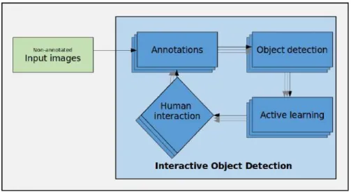
This is solved using a greedy procedure which iterates between minimizing the annota-tion cost and maximizing the accuracy of the object detecannota-tion model. Minimizing the annotation cost amounts to selecting a subset of non-annotated examples to be presented for feedback from oracle/human, as illustrated in figure 1.4. Maximizing the accuracy of the model amounts to tuning the object detector to all annotated examples. In this regard, the problem context, its scope and contributions are presented are follows.
Problem Context
While the importance of Active Learning for object detection is presented in section 1.1, the following are important practical considerations:
• Real-time constraints: A fundamental requirement to realize an effective Active Learning framework is to choose a suitable model for object detection. In such scenarios, the model must have the capability of fast training/testing times. Also,
Figure 1.4: Figure describing the architecture of Interactive Object Detection with
Active Learning. There is iteration between human interaction phase and object de-tection phase.
the model must be capable of learning from small/mid-sized datasets. In this regard, Hough Forests [30] is utilized as it has favourable runtimes, parallelizing potential and is shown to be robust to small/mid-sized datasets.
• Robust annotation cost: Another aspect of an effective Active Learning framework is to choose a robust annotation cost. The method [1] is adopted which is shown to be successful on real-world datasets and is inline with the Hough Forest model.
• Ease of verification: Finally, a simple user interface needs to incorporate verifica-tions from oracle/human in an effort effective manner needs to be realized.
1.3
Scope of this work
In this work, the focus is on developing real-time interactive object detection pipeline using Hough Forests for object detection and Active Learning. Overall the following challenges are solved.
• The problem of object detection can be challenging because of factors like view-point variation, scale variation, deformation, occlusion, illumination conditions, background clutter and intra-class variation as shown in figure 1.1 . The next problem in object detection is solving two problems of locating objects and classi-fying objects at the same time using the same model.
Both are solved using robust Hough Forests which uses deep features to defy view-point variation, scale variation, illumination conditions and intra-class variation. To solve both localization and classification problems, classification and regression nodes are incorporated in Hough Forests. Hough forests are explained in chapter 3
• The challenge in Active Learning is to find the most beneficial image to annotate, tuned to object detection problem.
Beneficial images to annotate in each iteration are found using uncertainty sam-pling based Active Learning method [1]. From the experiments, it is proved that Active Learning performs better than choosing random images. The Active Learn-ing method is explained in chapter 3 and experiments in chapter 5.
What is not in the scope of this work?
• Using deep learning methods for object detection: In this work real-time object detection is desired and deep learning based methods are slow to train.
• Multiclass detection is not incorporated in the Hough Forest-based object detector. Only one class of objects are detected per dataset.
• Comparision of different Active Learning query strategies ( explained in section 2.3) are not shown in this work. Only uncertainty sampling based Active Learning method is used for Active Learning.
1.4
Contributions
The contributions of this thesis are as follows:
• An Active Learning [1] framework for object detection [30] is realized.
• Traditional HoG features are replaced by state-of-the-art Deep features for im-proved object detection (See section 4).
• A Web-based annotation tool to incorporate verification from orcale/human is implemented.
• Custom implementation of Hough forests completely in Python, in comparison with C++ based implementation. Visualizations obtained through the custom implementation are shown in figure 3.2. The code is available in the CD attached.
• Qualitative and quantitative results on four Carl Zeiss/benchmark datasets is pre-sented.
1.5
Outline
The thesis is organised as follows:
State of the Art
In this chapter, popular approaches to solve the problem of object detection are ex-plained. Next, working with fewer annotated images, Interactive Learning and Active Learning are explained. State-of-the-art object detection methods, learning with par-tially annotated data and other Active Learning methods are explained to get a more relevant context.
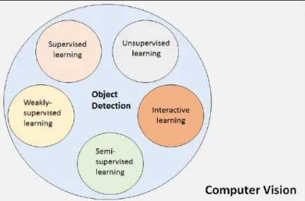
Interactive Learning method in the context of computer vision problem domain is shown in figure 2.1. Object detection is a sub-field of Computer Vision. Depending on the an-notation in the dataset, object detection can be solved using Supervised, Unsupervised, Weakly-supervised, Semi-supervised and Interactive Learning. In this work, Interactive Learning is focussed.
Combining the advantages of using deep learning and fast object detection based on Random Forests, method which uses deep features as an input to interactive object detector based on Hough Forests[1] is the main focus of this work.
2.1
Object Detection
The object detection algorithms combine the functional aspects of object location (where is the object?) [41] and object classification (which is the object?) [9] to detect objects.
2.1.1 Classical approaches
Earliest and most popular object detection method is using Haar features and cascade of classifiers [15] to detect faces. It uses Haar features [42] which are composed of five Haar templates. These features are extracted from a multi-scale sliding window. It uses Adaboost [43] for learning the cascade of classifiers. This was considered simple and
Figure 2.1: Interactive Learning method in the context of computer vision problem
domain. Object detection is a sub-field of Computer Vision. Depending on the anno-tation in the dataset, object detection can be solved using Supervised, Unsupervised, Weakly-supervised, Semi-supervised and Interactive Learning. In this work, Interactive
Learning is focussed.
fast by processing 15 frames per second and was used in point and shoot cameras which allowed real-time face detection.
Another method [44] uses Histogram Of Gradients features (HoG) and Support Vector Machines(SVM) [45] performed on a multiscale sliding window for person detection. HoG features were proved to be better than Haar features.
The next classical method to solve object detection problem with lesser parameters to tune in comparison to SVM is Random Forests [46]. The Random forest consists of an ensemble of decision trees arranged in a forest. Method [47] for face detection con-sists forests arranged in cascade structures influenced by method [15]. Another method Hough Forests [30] uses Hough Transform with Random Forests to detect generic shapes and object class instances. The input to the forest is HoG features extracted from im-ages. Each tree in the forest consists of randomly placed classification and regression nodes together performing detection. At the leaves of trees, the detection is performed by weighted aggregation of evidence from regression. Hough forests are used as the object detection component of this work’s Interactive Learning pipeline. This method is explained in detail in section 3.
Feature-based learning methods suffer from a problem that they only capture a small set of recognition cues and ignore other cues [48]. The features learned are image type specific and have to be re-learned for new image types. So there was a desire to develop algorithms to automatically learn features from images.
2.1.2 Convolutional Neural Networks
With improved computational power and large annotated datasets, the Convolutional Neural Network(CNN) paradigm today has largely been able to overcome the limitations of feature-based learning methods by automatically learning the features.
Regions with CNN features (R-CNN) [49] with CNN provided a 50% improvement over the best previous results on PASCAL VOC 2010 [50] dataset with feature-based meth-ods. It follows a three-stage approach involving first generating object proposals using selective search [51] method and feature extraction using CNNs, lastly classification us-ing SVMs. This method was slower because of CNN feature extraction applied to each proposal.
Quicker and modified approach Fast R-CNN [52] applied CNN to get features from the complete image instead of each proposal and then used both Region of Interest (RoI) pooling on the features with a final feed-forward network for detection. Usage of selective search slowed down the run-time of this method. In Faster R-CNN [53], a region proposal method was dropped to design a fully end-to-end trainable model. Also called Region Proposal network (RPN) it has a fully convolutional network which simultaneously predicts object bounding box and objectness scores for each position. An alternative paradigm is explored in You Only Look Once (YOLO) [24]. Unlike other object detection methods which use an intermediate object proposals stage, the method employs a single neural network to simultaneously regress the spatial extent of bounding boxes and its class label. This is performed by dividing the input image into cell grids and the regressing bounding boxes and confidence scores for each cell. The system used has 24 convolutional layers, 2 fully connected layers followed by a final layer which predicts class probabilities and bounding box coordinates. This predictor model is applied to an image at multiple locations and scales.
The next method called Single Shot MultiBox Detector (SSD) [13] combined the func-tional aspects of Faster R-CNN and YOLO. Object localistion and classification are performed in a single pass of the CNN. It is built on VGG-16 [53] base architecture with addition of auxillary convolutional layers to extract features from multiple scales and aspect ratios to compute confidence and location loss for classification and regression tasks respectively. Figure 2.2 shows working of SSD with an example. This is among the state-of-the-art, real-time object recognition systems.
All the methods mentioned above are based on Fully Supervised Learning approach which requires a lot of annotated data to reach their full potential. Next, methods which work with partially annotated data are explored.
Figure 2.2: SSD framework explained. a) and b) shows auxillary convolutional layers
with different scales (e.g. 8 ×8 and 4 × 4). For each auxillary convolutional layer, both the shape offsets and the confidences for all object categories (c1,c2,· · ·,cp) are predicted. Auxillary convolutional layers are matched to the ground truth boxes. For example, the two auxillary convolutional layers with the cat and one with the dog, which are treated as positives and the rest as negatives. The model loss is a weighted sum of
localization loss and confidence loss. Caption adapted from [13]
2.2
Learning with partially annotated data
2.2.1 Weak annotations
Given the difficulty in acquiring annotations, data annotation is a research area in itself. There are methods which make the job of annotations easier by introducing simplified annotation methods. In extreme clicking method [54], the bounding box annotations are provided in form of four points (xlef ttop,ylef ttop), (xrighttop,yrighttop),
(xrightbottom,yrightbottom),(xlef tbottom,ylef tbottom). This speeds up the process of annota-tion by 3x. In another method, object bounding-boxes are derived from eye-tracking [55] by fixations from eye movement of the annotators. In [56], detection is treated as a multi-stage problem. In the first stage, the user clicks on the centre of the object for annotating a bounding box. These annotations are used by Weakly-supervised object locations to localize the objects. These localised bounding boxes are used in next stage for detection. In semantic segmentation [57], annotating each pixel is a time-consuming task. Pixel-wise annotations are replaced by scribbles which is a user-friendly way of annotation.
Next, learning methods which work with partially annotated data are explored.
Weakly-Supervised Learning
Weakly-Supervised Learning [26, 58] makes use of image or instance level annotation for learning. This method is gaining popularity due to easily available image tags on images or videos, which can serve as image level annotations. With respect to object detection, the learning task is to localize and recognise the object using only image/instance level annotation but not the location of the object. This task is often termed as Weakly-supervised object localization (WSOL) [59]. The recent works in WSOL involving using
CNN to extract features improved the detection performance but it still slow compared to Fully Supervised Learning methods.
Semi-Supervised Learning
Semi-Supervised Learning [60, 61] makes use of small amount of annotated data with a large amount of unlabelled data. This has an underlying assumption of data being arranged in a cluster or along low dimensional manifolds. In self-learning method [62], the annotated data act as the base for object detector. The detections are propagated to unlabelled data and are further used to train the detector. There are chances that it becomes confidently wrong. In graph-based learning [63], the annotated data propagates the annotations to unlabelled data with a lower confidence. This is an iterative process which can go infinitely and can be difficult to scale. Max-margin and ensemble methods [64] develop a decision boundary based on the density of the mixture of annotated and unlabelled examples. These methods are usually tied to SVM based methods.
2.2.2 Transfer Learning
Due to the advent of CNNs, the knowledge (network weights) acquired from training very large datasets are transferred to learning unseen but related datasets. This transfer of knowledge is called transfer learning [65, 66]. This transfer could be done by using CNN as feature extractor or fine-tuning to already trained CNNs. This is, however, CNN method dependent and cannot be used with other methods.
2.2.3 Reinforcement Learning
Reinforcement Learning is learning policy based on reward or punishment. In the con-text of learning with partially annotated data, a policy for image annotation is learned instead of image analysis. In work [67] the agent is rewarded for actions that reduce the uncertainty about the unobserved images based on recurrant neural network to perform active completion of panoramic natural scenes and 3D object shapes. For the kind of data, setup and annotations present, this method cannot be used in our work due to the reason that the method is noise sensitive.
2.3
Interactive Learning
Interactive Learning is performed by a collaboration between human and machine for the process of learning. The interactive component can come from providing feedback by correcting annotations or providing new annotations, in each iteration. The user verification can be obtained for all images or a fixed number of images or for ”beneficial” images.
Incremental learning
In incremental learning [1], a fixed set of images for eg. everynthimage or randomly cho-sen image is annotated. These images are shown to the user via an interface to correct the annotations. In each iteration, an optimal threshold is computed to differentiate positive images from negative images. The order in which the images are annotated influences the detector’s performance. Therefore, in next method called active learn-ing, the images are selected in descending order of their difficulty to annotate. The comparison between Incremental and Active Learning is shown in figure 2.3
Active learning
A comprehensive literature survey related to Active learning is provided in [38–40]. Ac-tive Learning requires querying most beneficial images from the pool of data. Following are query methods :
• Random sampling
Also called Incremental Learning, in this method, a random image is chosen in every iteration instead of using any strategies. This strategy works best when the dataset contains similar images. But it can lead to learning of non-beneficial, repetitive images. The effectiveness of learning beneficial over random sampling is illustrated in figure 2.3. Random sampling is used as a baseline method in experiments section 5.
Figure 2.3: An illustrative example of the difference between Random and Active
Learning. (a) A toy dataset of 400 instances, evenly sampled from two class Gaussians. The instances are represented as points in a 2D feature space. (b) A logistic regression model trained with 30 annotated instances by picking random instances. The line rep-resents the decision boundary of the classifier (70% accuracy). (c) A logistic regression
model trained with 30 beneficial instances. Image and caption from [32].
• Query-By-Committee
This is an Active Learning method which queries form pool of unlabelled data. In each iteration, a committee of learning methods from the current training set is chosen. All the learning methods predict the output for each unlabelled image
in the dataset. The image whose prediction highly differs among the methods in the committee is selected to be annotated. The committee can be formed by same learning method with varying parameters [68] or by using ensemble learning [69]. Disagreement of the committee can be measured using vote entropy or KL divergence [70].
• Expected Model Change
In this method, the instance that results in the greatest change from the current model is selected for annotation in each iteration. One of the famous works using this method is [71] where, for each example of an unlabelled set, the expected change of model predictions is calculated and marginalized over the unknown la-bel. This results in a score for each unlabeled example that can be used for Active Learning with a Gaussian process for classification. This method could be ineffi-cient if both the feature space and set of labels are very large.
• Expected Error Reduction
In this method, the beneficial image is not selected on the basis of how the model is likely to change, but how the generalization error is reduced. The unlabelled pool of data is called validation set. If there is a highest decrease in generalization error on the validation set when an image is not used, this image is considered to be the beneficial image. In [72] a regressor is trained that predicts the expected error reduction for a data in a particular learning state. This method is computationally expensive because it requires estimating expected future error for each query and a new model must be incrementally re-trained for each query labelling which iterates over entire pool.
• Uncertainty Sampling
This Active Learning method queries an image whose annotation is most uncertain. The uncertainty can be decided on by the confidence obtained from score predicted by object detector [1] or entropy centred objective function as in [73]. It works on the concept that the image patches generated from the same object share the same label and differ slightly in their relative distance from the centre of the object. These patches will also have the same prediction from the learning method. The images having higher entropy generally indicate high variability among its patches. These images with higher entropy can contribute to increasing the performance of the learning method. The learning method used in this case is CNN. The Active Learning method used in this thesis [1] is based on uncertainty sampling method. It is explained in section 3. The disadvantage of using uncertainty based query strategy is that there is a possibility of learning noisy images because these kind of images have the highest uncertainty.
Further, deep learning is incorporated into Active Learning called ”Deep Active Learn-ing” [73] based on uncertainty sampling and CNNs. In [74] Bayesian Deep Learning is
to the object detector is HoG features obtained from images. The detailed explanation of this method is provided in Chapter 3. Figure 2.4 shows example output from Interactive Object Detection method from three datasets with images and with annotation cost. This work shows results on real-world datasets with fast object detection in order to perform interactive detection with user feedback.
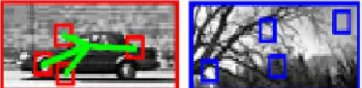
Figure 2.4: Results of the Interactive Object Detection framework for annotation from
work [1]. Green, red, and blue bounding boxes denote true positives, false positives, and false negatives respectively according to the annotation task. The numbers denote the predicted annotation cost, i.e., the cost to correct all detection errors in an image. The predicted annotation cost allows the user to select images for correcting detections and
Technical background
3.1
Hough Forests for object detection
Hough transform
Hough transform [1, 75, 76] can be used to find occurrences of a particular shape in images. The requirement is for the shape to be represented in parametric form. It was basically designed to find analytically defined shapes such as lines, circles and ellipsoids. For instance, here Hough Transform to detect lines can be shown in figure 3.1. In image space, a line can be expressed in cartesian co-ordinates with parametersρ,θ whereρ is the length of normal from the origin to the line to be found, andθis the orientation ofρ
with respect to the x-axis as: ρ=xcosθ+ysinθ. For a given (xi andyi) and (xj andyj) the family of lines that pass through this point are represented by: ρ=x0cosθ+y0sinθ as shown in figure 3.1 (a). Here, the observed variables are from R ∈ (xj, yj) and parametric space isR∈ (ρ, θ)
Figure 3.1: Simple example of Hough Transform. A line shown in (a) is transformed
into curve shown in (b).
The possible values of (ρ,θ) are plotted against specific (xi and yi) and (xj and yj) , values in cartesian image space, to curves in polar Hough parametric space. This transformation is called Hough Transformation for lines. This allows for efficient and robust implementation which is occlusion, noise and deformation independent.
(ρ,θ). Each value (xi,yi) and (xj , yj) is transformed into discretised (ρ,θ) curve and all the bins along this curve are aggregated as shown in figure 3.1 (b). The peaks in Hough space bins represent the presence of a line. As there could be multiple possible aggregated bins, the useful peaks are found by non-maximal suppression [77]. Hough transform is extended to detecting other shapes which are analytically defined shapes and object class instances [30][78].
Generalised Hough Transform
Hough transform can be applied for detection of any shape based on aggregation of evidence of the presence of the transformed curve with respect to the image of interest [30]. These evidences are called ”Hough votes” The parametric space here is called ”Hough space”. The parameters here can be set of object location in image, scales, aspect ratios etc. The detection step is finding peaks of aggregation of Hough votes in Hough space by non-maximal suppression. Next, how Hough Transform is used with Random Forests to detect objects is presented.
Random forests with generalised Hough Transform
The previous research work is re-iterated here to explain random forests [29]. Hough forests are a group of decision trees.
Random forest [46] is an ensemble of decision trees [79]. Decision trees are the hier-archical tree-like representations consisting nodes and branches. During decision tree learning, it looks into attributes in data to split the data into subsets. Splitting is done according to different criteria like Gini impurity, regression or entropy loss. Here binary tests are used to determine the best splits. The splitting is continued until the subsets are pure and the results are stored in the leaf node. One disadvantage of decision trees is it can easily over-fit the data. Random forests, on the other hand, is an ensemble of decision trees whose input is a random subset of the actual data. The final result of the random forest is the mean or mode of the result of individual decision trees.
The following equations are used as is and explanations are adapted from work [1, 30, 80]. In the Hough Forests implementation used from [30, 80], the features from the image are mapped to corresponding votes in Hough space. ydenotes the mid-point of input image patch with dimension D. The features are denoted by (I1(y),I2(y),....If(y)) where F
denotes the number of feature channels. Idenotes mapping from the patches to features. In work [30], this mapping is done by HoG and RGB features. H denotes Hough space and h denotes hypothesis.
The leaves of the trees{L}model the mapping from the patch with centre y to proba-bilistic Hough vote denoted by:
L: (y,I)−→p(h|L(y)) (3.1)
p(h|L(y) is the distribution of Hough votes in Hough space. Learning mappingL is also learning Hough Forest model which is explained in next section.
3.1.1 Training
The trees are trained on image patches. For each class, c ∈ C training images are available. Positive image patches are sampled from inside bounding box and negative patches are sampled from the background as shown in figure 4.1. Each patch contains information regarding its class. In addition, each positive patch also contains information about offset from the centre of the patch to the centre of the object. TheD-dimensional image is used to build Hough tree T and forest T = {Tt} from the set of patches
{Pi= (Ii, ci,di)}where di is offset vector.
The tree consists of leaf and test nodes. Each non-leaf node is assigned a binary test whose domain are the features Ii = (Ii1, Ii2....IiF). A binary test tθ(Ii) on a patch is parametrised by θ = { f, p, q, τ } where f ∈ 1,2,3, ..., F is generated on two randomly chosen positionsp ∈RD andq∈RD within feature matrix and a real-valued threshold τ. The test is:
tθ(Ii) =
(
0 if Iif(p)< Iif(q) +τ,
1 otherwise (3.2)
The evaluation criteria for the binary test is to minimise the uncertainty for either discrete or continuous random variables which are class labels cand offset vectors d. Each non-leaf node in the tree is either classification (to minimise the uncertainty of class label) or a regression node (to minimise the uncertainty of offset vectors) decided randomly. Let P be set of incoming patches. For a classification node, the measure of the uncertainty of set of patches is given by:
U1(P) =− |P| X
c∈C
p(c|P) ln(p(c|P)) (3.3)
where |P| is the number of patches in set P and p(c|P) is the proportion of patches with labelc inP. Minimising this expression for a node corresponds to maximising the information gain.
At each node, a pool of binary tests { θk } are generated with random values of f, p,
q and τ sampled uniformly. Binary test θ for a test node is chosen in a greedy fashion from a set {θk}. All the patches arriving at a node are evaluated for the set of binary tests θk and the best binary set is chosen and stored at the node. Best test should minimise the following minimization objective:
argmin
k
(U∗({Pi|θk= 0}) +U∗({Pi|θk = 1})) (3.5)
where∗ indicates uncertainty measure for classification (U1) or regression (U2).
To construct a leaf node L , information from incoming patches are used to store the class probabilityp(c|L) and a list of offset vectors DL
c = {di}ci=c.
The tree is constructed recursively starting from the root by choosing a binary test and children nodes are constructed until a stopping criterion is reached. The stopping criteria could be the tree reaching its maximum depth (in our case 15 trees) or the number of patches falling below a threshold (in our case 2). When one of this criterion is met, leaf nodes are constructed with information of class probabilitiesp(c|L) and list of offset vectors D = {di}ci=c. One example of a trained Hough Forest with depth 3
can be seen in figure 3.2 where the image patches are fed into Hough Forests and they traverse in the forest splitting in regression or classification node to reach leaf where offset vectors and the probability of positive patches are stored. In the figure, the positive and negative patches are fed into the root of the tree. The first node is a classification node which differentiates negative patches from positive patches. The right child is also a classification node. The left child is a regression node which differentiates front part of the horse and back part of the horse. At the leaf nodes, as shown in the last row, the class probability p(c|L) and a list of offset vectors DcL = {di}ci=c centered at the red
point are stored.
3.1.2 Testing
During detection phase as shown in figure 3.3, the test image patches pass through each tree in Hough forest. The leaves that the patches arrive cast votes in Hough space H. The Hough space is composed of parameters image scale and position.
Let a patch with the centre at position y be Py = (Iy, cy,dc(y)) ∈ Ω ⊆ RD in the test image. Here Ωis set of all pixel locations, Iy is the set of observed features of the patch,
is a regression node (in red) which differentiates front part of the horse and back part of the horse. At the leaf nod probabilityp(c|L) and a list of offset vectorsDL
Figure 3.3: For each of the three patches emphasized in (a), the pedestrian
class-specific Hough forest casts weighted votes about the possible location of a pedestrian (b) (each colour channel corresponds to the vote of a sample patch). Note the weakness of the vote from the background patch (green). After the votes from all patches are aggregated into a Hough space (c), the pedestrian can be detected (d) as a peak in this
image. Caption and image from [1]
cy is the hidden class label and dc(y) is the hidden displacement from the patch to the unknown object’s centre. Based on the feature Iy , patch Py ends in a leaf L(y). Let h be the hypothesis for the object belonging to class c with size s and centered at x ∈ Ω. The conditional probability p(h(c, x, s)|L(y))can be computed as
p(h(c,x, s)|L(y)) =X l∈C p(h(c,x, s)|c(y) =l, L(y))·(c(y) =l|L(y)), =p(h(c,x, s)|c(y) =c, L(y))·(c(y) =c|L(y)), =p x=y− s su d(c)|c(y) =c, L(y) ·p(c(y) =c|L(y)), (3.6)
where su is the unit size of the training data. p(c|L) is estimated as the proportion of patches per class label reaching the leaf after training, the distributionp(h(c, x, s)|c(y) =
c, L(y))can be approximated by a sum of Dirac measuresδd for the displacement vectors
d ∈DLc : p(h(c,x, s)|L(y)) = p(c(y)) =c|L(y) D L(y) c X d∈ D L(y) c δd su(y−x) s (3.7)
For the entire forest T, features of the patch are passed through all the trained trees and average the probabilities from equation 3.7 from different leaves:
p(h|Iy) = 1 T T X t=1 p(h|Lt(y)), (3.8)
whereLt(y)is the corresponding leaf for tree Tt. The votes from all patches of the image are accumulated in the Hough space H:
p(h|Iy) =
X
y∈Ω
p(h|Iy) (3.9)
The modes of p(h|I) can be obtained by searching for local maxima using a Parzen estimator with a Gaussian kernel K:
ˆ p(h|I) = X h′∈h w′h·K(h−h′), where wh′ =X y∈Ω |T | X t=1 X d∈Dt(y) c p(c(y) =c|Lt(y)) D Lt(y) c δd su(y−x) s (3.10)
The weight of a hypothesisw′haccumulates votes that support similar hypothesesh′(c, x, s)
∈ H. After all votes are cast,pˆ(h|I) represents the sum of the weights of the hypotheses
in the neighbourhood ofhweighted by a Gaussian kernelK. While the location of a local
maximum hˆ(c, x, s) encodes class, position and size of the object, the value of pˆ(ˆh|I) is
not a probability but serves as a confidence measure for each hypothesis.
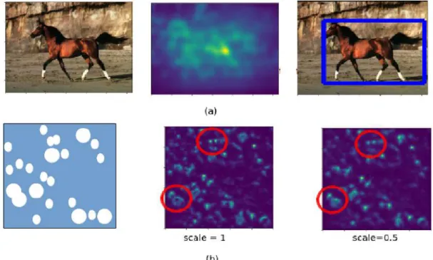
Example detection from the experiments conducted is shown in figure 3.4. Figure 3.4 (a) shows original image, with its Hough space and next detection by non-maximal suppression. And figure 3.4 (b) shows Hough space obtained for different scale which detects the objects having different scales, the first Hough space with scale=1 detects smaller objects and second Hough space with scale=0.5 detects bigger objects.
3.2
Active learning
Threshold estimation
In this section, implementation of Active Learning along with Hough Forests is described. Hough forest provides a score for each bounding box (hypothesis) detected. These scores can be thresholded to accept or reject the bounding box.
During Hough Forest detection, the positive and negative hypothesis needs to be distin-guished using the bounding box scores. The detection scores corresponding to positive hypothesis are denoted by Spos and scores from negative hypothesis denoted by Sneg. The distribution of scores conditional to a positive or negative hypothesis is denoted by p(s|pos) and p(s|neg). These conditional probabilities are modelled well by Gamma distributions [81]:
Figure 3.4: Testing part of Hough Forests explained with an example. (a) The
Orig-inal image, with its Hough space and next detection by non-maximal suppression. (b) Synthetic dataset image with Hough space obtained for different scale detects the ob-jects having different scales, the first Hough space with scale=1 detects smaller obob-jects
and second Hough space with scale=0.5 detects bigger objects
k and θ are the parameters of the gamma distributions obtained from Spos and Sneg. The optimal threshold is formulated as that value of threshold τ which minimises the probability of false positive F P and false negative F N hypothesis for a given τ. This can be mathematically written as:
argmin
τ
p(F P|τ) +p(F N|τ) (3.12)
based on above equations, following equations can be formulated:
p(F P|τ) =p(neg) Z ∞ τ p(s|neg)ds (3.13) p(F N|τ) =p(pos) Z τ 0 p(s|pos)ds (3.14)
wherep(pos) = |Spos|
|Spos|+|Sneg| and p(neg) = 1−p(pos). The initial threshold is calculated
to be median of all the positive and negative hypothesis scores.
For every new score, the parameters of gamma distribution are updated. Initial threshold estimation requires at-least two annotated images. With more training examples, a
better threshold can be estimated. The initial threshold is higher and converges after few iterations as shown in figure 3.6.
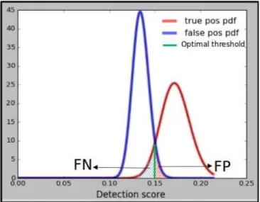
In figure 3.5 which shows gamma probability density function(PDF) of the scores, the intersection of two PDFs shows the scores which are most uncertain ie. false positive scores (red hashed regions) and false negative scores (blue hashed regions). The score which clearly distinguishes the false positive scores from false negative scores is consid-ered optimal threshold (green line).
Figure 3.5: Detection scores of positive (blue) and negative (red) detection scores
modelled by the gamma distribution. These distribution parameters are updated after each incremental training step. false positive scores (red hashed regions) and false negative scores (blue hashed regions). The score which clearly distinguishes the false positive scores from false negative scores are considered optimal threshold (green line)
Annotation cost
As the order of annotating images is responsible for the quality of detections, next Active Learning way of interactive detection is explored. Here the most beneficial images which have highest annotation cost is selected to annotate first. The annotation cost is formulated as: fpred(S, τ) =X s∈S p(F P|s, τ) +p(F N|s, τ) (3.15) and p(E|s, τ) = p(s|E, τ)p(E|τ)
p(s|neg)p(neg) +p(s|pos)p(pos) (3.16) whereE ∈F P, F N and p(s|F N, τ) = ( 0 if s≥τ p(s|pos) Rτ 0 p(s|pos)ds if s < τ (3.17)
hashed region in the figure comprises the scores which are most uncertain. The equation 3.16 finds the image for which the area of uncertainty of all its scores is very high. Thus, during every iteration of Active Learning, an image with highest annotation cost is found. For this image, the annotation from the user is obtained and the iteration is continued until the stopping criterion is reached. The stopping criterion is when the annotation cost is 0 as shown in figure 3.6.
Figure 3.6: Convergence of (a) optimal threshold and (b) annotation cost over 10
iterations
Algorithm 1 Active learning algorithm
1: procedure getBeneficialImage(images)
2: τ ←median(prevsScores)
3: S ←houghF orestP redict(images) 4: maxAnnotationCost←0 5: for s in Sdo 6: if s≥τ then 7: Spos =s 8: else 9: Sneg =s 10: p(pos)← |Spos| |Spos|+|Sneg| 11: p(neg) = 1−p(pos)
12: kpos, θpos =getGammaP aram(Spos) 13: kneg, θneg=getGammaP aram(Sneg) 14: minτ =min(S)
15: maxτ =max(S)
16: τlist=unif orm(minτ, maxτ,100) 17: for τ in τlist do
18: R∞
τ p(s|neg)ds=gammaCdf(t, kpos, θpos)
19: Rτ
0 p(s|pos)ds=gammaCdf(t, kneg, θneg)
20: p(F P|τ) =p(neg)R∞
τ p(s|neg)ds
21: p(F N|τ) =p(pos)Rτ
0 p(s|pos)ds 22: for S, image in imagesdo 23: annotationCost= 0 24: fors in S do 25: if s≥τ then 26: p(s|F N, τ) = 0 27: p(s|F P, τ) = pR(∞F P|τ)p(neg) τ p(s|neg)ds 28: else 29: p(s|F P, τ) = 0 30: p(s|F P, τ) = pR(F Nτ |τ)p(pos) 0 p(s|pos)ds 31: p(F P|s, τ) = p(s|F P,τ)p(F P|τ)
p(s|neg)p(neg)+p(s|pos)p(pos) 32: p(F N|s, τ) = p(s|F N,τ)p(F N|τ)
p(s|neg)p(neg)+p(s|pos)p(pos) 33: annotationCost+ =p(F P|s, τ) +p(F N|s, τ) 34: if annotationCost≥maxAnnotationCost then 35: maxAnnotationCost=annotationCost 36: benef icialImage=image
This chapter presents implementation details of the Hough Forests, the Active Learning framework and the web-based annotation tool used to gather annotation from oracle/hu-man.
4.1
Hough Forest
As discussed in section 3, Hough Forests uses generalized Hough Transform for generic shapes/objects. The details of its components are described in following sections.
4.1.1 Patch extraction
The input to all experiments is RGB images and ground truth bounding boxes of positive examples. In order to simplify the training procedure, positive bounding boxes are rescaled to its median value. Testing is performed in scale space, corresponding to the modes of scale distribution in the training data.
Patch extraction
The input to Hough Forests are patches of fixed n×n size patches extracted from the training images. The size of the patches is fixed as 16 × 16. Positive and negative patches are randomly sampled from within and outside the (scaled) positive examples respectively. Instead of using just the RGB image patches, a simplified image
represen-Figure 4.1: Positive patches extracted from inside bounding box and negative patches
extracted the from the background.
tation which consists of ”useful” components from images, also called features, are used. The features are designed to contain colour, edge, corner and texture information. E.g., while RGB-only patches contain colour information, Histogram of Oriented Gradients (HoG) features capture structured edge information and Deep features capture edge and texture information.
RGB features
RGB features are composed of R, G and B channels of the image. These are simplest features having pixel intensity values for each colour channel. Here the features are the images itself.
HoG features
HoG features have shown [44] to be state of the art features for object detection until the advent of data-driven (deep) features. HoG features retain shape information by capturing edge information. Due to localized normalization and binning, it is robust to local variations in illumination and articulation. The distribution of directions of gradients is used as HoG features. Gradients (horizontal and vertical) of an image are useful because the magnitude of gradients is large around edges and corners which are the regions of abrupt intensity changes. Therefore, edges and corners contain valuable information about object shape.
HoG feature extraction is a three-step process: During the first step, first the horizontal,
gx and vertical, gy gradients are calculated. This is achieved by filtering the image with the Sobel [82] filters. The gradient image has a high response at edges or object boundaries and low response in uniformly coloured regions. Next, The magnitude and direction of the gradient is computed as
g=qg2 x+gy2
θ=arctangy gx
(4.1)
Whereg is the gradient magnitude andθis the gradient direction. As for colour images, the maximum gradient magnitude among the three channels and the corresponding gradient direction is retained.
During the second step, the image is divided into 8×8 cells and a histogram of gradients is calculated for each 8×8 cell.
In the final step, features are normalised to be independent of local lighting variations. This is illustrated in figure 4.2. The figure shows the nine channelled HoG features with (a) showing all horizontal gradients, (b) incorporating neck highlighting gradients, (c) incorporating face and leg highlighting gradients, (d) incorporating face and leg high-lighting gradients, (e) incorporating vertical gradients, (f,g,h) incorporating body and
Figure 4.2: The figure shows the nine channelled HoG features of input figure A.1
(a) showing all horizontal gradients, (b) incorporating neck highlighting gradients, (c) incorporating face and leg highlighting gradients, (d) incorporating face and leg high-lighting gradients, (e) incorporating vertical gradients, (f,g,h) incorporating body and some background highlighting gradients and (i) incorporating background highlighting
gradients.
Deep features
Deep features are extracted using Convolutional Neural Networks (CNNs) which produce hierarchical trainable features. These are robust [9] compared to handcrafted HoG features. The layers of CNN have three dimensions - width, height and depth (activation volume). CNNs make use of the property that if one filter is used to compute some feature, then the same filter should also be useful to compute similar feature at a different position. This property, called parameter sharing, also makes CNNs translation invariant by detecting features regardless of their position in the image. CNNs also take into
consideration that images are spatially locally correlated by having a local connectivity pattern between neurons of adjacent layers. The CNN consists of multiple convolutional, rectified linear unit, pooling, dropout and fully connected layers. In this work, features are extracted from the convolutional layer.
The convolutional layer consists of kernels/filters which have a receptive field. During forward pass, the filter convolves around the image computing the dot product between the entries of the filter and the input producing 2-dimensional ”activations” of the filter. These filters learn specific features which activate when similar features are found else-where in the image. There can be many such filters in a convolutional layer. Stacking these ”activations” for all filters along the depth dimension forms the full output of that convolution layer. Visualization of the Convolutional layer’s filters can be seen in figure 4.3 and activations in figure 4.4.
Figure 4.3: The input image on left and visualization of the Convolutional layer’s
filter on right.
The convolutional layer can have hyper-parameters like Receptive field F or size of the filter, the number of filters K and Stride S with which filters slide. When the stride is 1, then filters are moved one pixel at a time, Size of zero-paddingP padding the input volume with zeros around the border. It allows us to control the spatial size of the output of the filter.
If the filter receives an input volume of size W1×H1×D1, it produces a volume of size W2×H2×D2 where: W2 = W1−F+ 2P S + 1 H2 = H1−F + 2P S + 1 D2 =K (4.2)
With parameter sharing, it introduces F ×F ×D1 weights per filter, for a total of (F ×F ×D1)×K weights and K biases. In this work, VGG19 model trained on
Figure 4.4: Visualization of the Convolutional layer’s activations.
Imagenet [9] dataset is used. The features are extracted from the second convolutional layer of this VGG model as shown in figure A.2.
4.1.2 Training
During the training of Hough forests, number of trees and depth of each tree was fixed at 15. The effect of changing these parameters are explained in section 5. The number of tests per each non-leaf node in the tree was fixed to 2000. The non-leaf nodes were randomly chosen to be classification or regression nodes. In each leaf, the class proba-bility and a list of offset vectors are stored. The patch size of the patches extracted from the images from the datasets are fixed to height and width of 16 pixels. The number of patches extracted per image is dependent on the dataset chosen. The stopping criteria for training is when the maximum depth is reached or the number of patches reaching the node is smaller than 2.
4.1.3 Testing
During testing, patches are extracted from the entire test image in multiple scale space. The number of scales is different for different datasets which are dependent on the variety of object shapes present. To find the peaks in Hough space, non-maximal suppression
[83] is performed to findnpeaks fornobjects. The number of objectsnis pre-determined depending on the dataset.
Bounding boxes from Hough space
The bounding box height and width is fixed to be median of height and width of all bounding boxes seen during training. For each scale, the bounding boxes are rescaled accordingly. After non-maximal suppression performed for each peak, a detection is bounding box with centre at the peak.
4.2
Interactive Learning stage
As discussed in section 3, the Active Learning framework is initialized by annotating two images. The first image is used to seed the Hough Forest-based object detector. The scores from the second image are used for seeding the Active Learning phase. The Active Learning pipeline is implemented as a procedure illustrated in figure 4.5 and steps are as follows:
1. The dataset for Active Learning is chosen.
2. 20% of the dataset is held out for testing and 80% of the dataset is held out for training.
3. Two annotated images or positive images and two negative images (the images which do not contain the object of interest) are selected to train.
4. Interactive detection begins by training on two positive and two negative images. 5. Active learning is performed using bounding box scores obtained by rest of the
training images and trained forest model.
6. A beneficial image is chosen from rest of the images whose annotation cost is highest and used for re-training.
7. Evaluation is performed on evaluation images with the trained forest model. 8. Steps 4 to 7 are repeated until the annotation cost is zero.
4.3
Evaluation measure
Object detection
The evaluation metric for object detection is mean Average Precision (mAP). This is calculated as the area under the interpolated precision and recall curve.
Figure 4.5: The Active Learning evaluation pipeline showing steps during Active
Learning and evaluation. In step 1, the dataset is obtained. In step 2, the dataset is divided into training and test images. In step 3, two annotated images and two unlabelled images are selected to train. In step 4, 5 and 6, training, active learning and
evaluation are performed iteratively until stopping criteria is reached.
Actual class Predicted class
Positive class Negative class Positive class True positive False positive
Positive class False negative True negative
Table 4.1: True/False Positive and Negative definition.
To calculate precision and recall, first True Positives, False Positives and False Negatives are evaluated. This is evaluated by using the Intersection over Union (IoU) metric where True Positives have IoU ≥ 0.5, False Positives have IoU < 0.5 and False Negatives are un-detected object instances. The definitions are tabulated in table 4.1. The IoU between a detected bounding boxdand a ground-truth bounding box gis calculated as
IoU(d, g) = d∩g
d∪g (4.3)
whered∩gandd∪g are areas of intersection and union between bounding boxesdand
Figure 4.6: Figure showing a graphical illustration of Intersection of Union (IoU) and
random bounding boxes with IoU of 0.25, 0.5, 0.75 and 0.97.
Precision is calculated as the fraction of positive detections among all detections: Precision = True Positive
True Positive + False Positive (4.4) and recall as the fraction of positive detections among all possible positive detections:
Recall = True Positive
True Positive + False Negative (4.5) the precision-recall curve shows the tradeoff for varying thresholds of voting confidence. A high value of the area under the curve shows both high recall and high precision. A high precision value corresponds to low false positive detections and high recall value corresponds to low false negative detections. If a model has a high recall and low precision it results in many detections but most of its detections are incorrect. If a model has high precision and low recall it results in few but correct detections. Ideal object detection model has high precision and recall which results in many and correct detections.
The mAP is then calculated as the area under the interpolated precision-recall curve, as illustrated in figure 4.7 (hashed region).
Active learning
The effectiveness of Active Learning is found by comparing Active Learning to incremen-tal/passive learning where new samples to be annotated are selected randomly. Further, Active Learning experiments are performed until stopping criteria, i.e. when the anno-tation cost is zero, is reached.
Hard Negative mining
A popular trick of boosting object detection performance is to incorporate hard negative mining [84]. Here, false positives from the previous iteration are added as negative examples during training the model in the present iteration. This helps the Hough
Figure 4.7: Interpolated precision-recall curve for example iteration.
Forest to distinguish between real positive samples and difficult negative samples. This technique is incorporated in all experiments discussed in section 5.
4.4
Adaption in web annotation tool
To obtain annotations from the user in every iteration, a web-based annotation tool is developed. It is adapted from [85] using Python [86] programming language and Flask framework [87]. The snapshot of the tool is shown in figure 4.8. It has the following functionalities
1. ”Start” experiment by loading two images.
2. Annotate object of interests with ground truth bounding boxes. 3. Download the annotations and ”Train” the Hough Forests. 4. Perform Active Learning using ”Test” button.
5. Load the beneficial image.
6. Repeat steps 3-5n times to annotate n beneficial images.
To the available annotation application, the functionality of Active Learning has been added. In figure 4.8, the top black task bar has ”Start” button to load first two images.
The image annotation is done using the left side tool bar by choosing the annotation bounding box of our interest. The shape of the bounding box used is the rectangle. The annotated images are trained using the ”Train” button on the top black task bar. For the completely annotated datasets, a graph with mAP for the trained images is shown below the black task bar (not shown in the figure). The graph also shows the comparison of mAP of Fully Supervised, Passive and Active Learning. The graph is updated every time after training. Active learning is performed by clicking on ”Test” button on the top black task bar. ”Load” button is used to load the beneficial image which can be used in next training and Active Learning iteration. The code for this tool is available in the CD attached.
Evaluation
In this chapter, details of the datasets, experimental analysis, qualitative and quantita-tive results are presented.
5.1
Experimental setup
5.1.1 Datasets
Four datasets are considered for experimental evaluation of Active Learning and object detection. Two of these datasets are standard benchmark datasets used in the com-puter vision community. The Weizmann Horse [88] is a relatively small RGB-dataset containing horses as the object of interest. The PASCAL VOC 2007 [89] dataset is closer to a medium-sized real-world RGB-dataset. The class ”car” is considered for experimental evaluation as shown in [30]. Both datasets come bundled with ground truth bounding box annotations. Sample images from both datasets are illustrated in figure 5.4 and figure 5.8. The next two datasets are custom Carl Zeiss datasets. CZHisto is a Histopathology RGB-dataset where objects of interest are steatosis cells. Finally, CZHeLa [90] is a dataset captured by a Focussed Ion Beam -Scanning Electron Micro-scope (FIB-SEM) of cervical cancer HeLa (Henrietta Lacks) cell where objects of interest are mitochondria. Sample images from this dataset are illustrated in figure 5.14. Each image is a single-channel image stack. Ground truth annotations for these datasets were obtained through manual annotation. The properties of various datasets are summarized in table 5.1.
The scale variations for the four datasets are shown in figure 5.1. For each dataset, the median of minimum value among height and width of the bounding boxes is found. In the figure 5.1, all the plots show median - 50% to median + 50% of scale variations. The plots which have Gaussian nature represent lesser scale variations and others represent higher scale variations. Clockwise, the first plot shows the scale variations for Weizmann Horse
Carl Zeiss datasets CZHisto 600 steatosis cells ∼15 yes unclear object boundaries
CZHeLa 120 mitochondria ∼20 grayscale scale variations
Table 5.1: Characteristics of datasets used in the experiments.
dataset. Second shows the scale variations for PASCAL VOC 2007 dataset. Third shows scale variations for CZHeLa dataset and fourth shows variations for CZHisto dataset. Among all the plots, PASCAL VOC 2007 shows highest scale variation and is also the most difficult dataset.
Figure 5.1: All the plots show the scale variations from median - 50% to median +
50% of scale variations. The plots which have Gaussian nature represent lesser scale variations and others represent higher scale variations. Clockwise, the first plot shows the scale variations for Weizmann Horse dataset. Second shows the scale variations for PASCAL VOC 2007 dataset. Third shows scale variations for CZHeLa dataset and fourth shows variations for CZHisto dataset. Among all the plots, PASCAL VOC 2007

![Figure 1.3: Interactive Learning cycle. Image adapted from [32]](https://thumb-us.123doks.com/thumbv2/123dok_us/1364141.2682627/13.892.267.692.203.449/figure-interactive-learning-cycle-image-adapted.webp)
![Figure 2.4: Results of the Interactive Object Detection framework for annotation from work [1]](https://thumb-us.123doks.com/thumbv2/123dok_us/1364141.2682627/24.892.224.725.369.670/figure-results-interactive-object-detection-framework-annotation-work.webp)