Improved density peak clustering for large datasets

HAL Id: hal-01353574

https://hal.archives-ouvertes.fr/hal-01353574

HAL is a multi-disciplinary open access archive for the deposit and dissemination of sci-entific research documents, whether they are pub-lished or not. The documents may come from teaching and research institutions in France or abroad, or from public or private research centers.

L’archive ouverte pluridisciplinaire HAL, est destinée au dépôt et à la diffusion de documents scientifiques de niveau recherche, publiés ou non, émanant des établissements d’enseignement et de recherche français ou étrangers, des laboratoires publics ou privés.

Improved density peak clustering for large datasets

Vincent Courjault-Rade, Ludovic d’Estampes, Stéphane Puechmorel

To cite this version:

Vincent Courjault-Rade, Ludovic d’Estampes, Stéphane Puechmorel. Improved density peak cluster-ing for large datasets. 2016. �hal-01353574�

Improved density peak clustering for large

datasets

Vincent Courjault-Radé

Université fédérale de Toulouse, ENAC

F-31055 Toulouse, France

and

Ludovic d’Estampes

Université fédérale de Toulouse, ENAC

F-31055 Toulouse, France

and

Stéphane Puechmorel

Université fédérale de Toulouse, ENAC

F-31055 Toulouse, France

August 12, 2016

Abstract

Clustering is the usual way of classifying data when there is no a priori knowledge, especially about the number of classes. Within the frame of big data analysis, the computational effort needed to perform the clustering task may become prohibitive and motivated the construction of several algorithms or the adaptation of existing

ones, as the well known K-means algorithm [12]. Recently, Rodriguez and Laio [17] proposed an algorithm that clusters efficiently by fast searching local density peaks that are sufficiently distant one from the others. However it is able to work on small datasets only and is highly sensitive to the value of tunable parameters. In this paper we propose Improved Density Peak Clustering (IDPC), a new algorithm designed for large datasets based on [17] which corrects the shortcomings mentioned above. Thanks to our Cover Map (CM) procedure iterated with a decreasing locally-adaptive window (ICMDW), we are able to build both a localisation map and a multidimensional density map. The nature of the density map, which fits perfectly with the approach of [17], allows us to compute the different steps with much less operations. It carries unsensitive parameters, supports last improvements on cluster centers selection and potentially allows new improvements.

Keywords: Clustering algorithm; density-based clustering; large datasets;

1

Introduction

Clustering is a commonly used tool that aims to identify similar samples in a dataset. It can be viewed both from the machine learning and the statistics point of view, with classical algorithms pertaining to each domain. When considered from the algorithmic standpoint, the complexity of the clustering problem is known to be NP hard, even for the usual K-means, when the number of clusters is not fixed.

Presented in [17], the innovative fast density peak detection (FDPC) algorithm is able to cope with non-convex clusters and gives a convenient decision rule to find the correct number of clusters. As in the mean shift algorithm [3], clusters centers are defined as local density maxima. More specifically, a cluster center is defined as a point surrounded by neighbours with lower local density and away from any other local maxima. In order to detect them, a distance dc is first selected and is used to define neighborood. Densities ρi are calculated at each data point xi by counting the number of sample points closer than

dc to xi (1). Next, for each data point, the nearest point with a higher density is found and the distance δi separating them is recorded (2). Cluster centers are then defined as the points xi that have both high density ρi and high distanceδi. Other points receive the same label than their nearest neighbor of higher density (3).

This innovative method has promising results but shows some limitations. In step (1), the distances between all sample points are calculated, leading to an O(N2_{) complexity} and memory footprint, not to mention other steps. This issue limits it to small datasets. Furthermore, choosing a good threshold distance dc is non-trivial and critical since it has a major impact on the final clustering.

Our new algorithm aims to overcome the drawbacks mentioned above. The general idea of IDPC is to start by the construction of a density map trough the procedure Iterated Cover Map with a Decreasing Window (ICMDW), reducing the dimension N of the problem, and then to use the localisation information it provides to construct a very fast version of steps (2) and (3).

In the second Section we review the work related to [17]. In the third Section we detail the implementation of the ICMDW algorithm. In the fourth Section we explain how the results provided by ICMDW are used to greatly reduce the computations in cluster centroid selection and labelisation. And finally, we present experimental results in the fifth Section.

2

Related work

2.1

Fast Density Peak Clustering

Let (xi)i=1...N be the sample points. In the first step of FDPC the Euclidean distances dij between each data points are computed. Then a distance dc is chosen to finally compute, for eachxi, the number of data points that are closer thandcto the pointxi. Local densities

are then obtained according to the formula: ρi :=ρ(xi) = N X j=1 (1_R−(d_ij −d_c)).

Please note that the expression is of the form PN

j=1K(xi−xj), where K is the so-called kernel function, that reduces here to the characteristic function of a ball 1B(0,dc).

In the second step, the minimum distance between the point xi and any other point with higher density is calculated asδi = minj:ρj>ρi(dij). Finally, cluster centers are found as

out-liers in the decision graph formed by (δ, ρ), where outliers are the points sharing anoma-lously large density-delta values. Conventionally, for the point xk with highest density,

δk = maxj(dij).

Finally, other points are assigned to the same cluster than their Nearest Point with Higher Density (NHPD). Its algorithmic is detailed in Algorithm 1.

Many researchers worked on this algorithm in order to improve and/or use it on a specific

Algorithm 1 FDPC procedure F DP C(dc) for all (i, j)∈ { 1, ..., N}2 _do dij ←distance(xi, xj) end for for all i∈ {1, ..., N} do ρi ← PN j=1(1x<0(dij −dc)) end for for all j ∈ {1, ..., N} do nhpd_j ←argmin_{k:ρ(xk)>ρ(xj)}(djk) δj ←dj,nhpd_j end for

Cluster centers ← outliers in decision graph

∀j, Labelj ←Labelnhpd_j end procedure

problem. It has been used successfully on clustering of electricity consumption behaviour [22], text clustering [10], unsupervised acoustic subword units discovery pompage [25], batch process modelling and on-line monitoring [16], medical data [7] and it has been

slightly modified to work on image segmentation [1, 2, 18], outliers detection [4] and hyper spectral band selection [6]. K-means and FDPC have been compared in [15] and FDPC has shown more accurate than K-means.

However, FDPC has proved to be slower than K-means and suffers from three other shortcomings:

• First of all, due to its inherent computational complexity, it cannot handle large data sets.

• Secondly, the choice of dchas to be made empirically whereas it highly impacts every steps of the clustering algorithm.

• Finally, no decision rule is given to determine the outliers in the decision graph, leading to a manual or poor automatic selection of the cluster centers.

2.2

Improvements of FCDP

To overcome the limitations underlined above, a lot of work was done to derive improved versions of the original algorithm. Most of them deals only with one issue, due to the application:

Ability to handle large datasets

An extension of FDPC [9] has been proposed in order to manage large taxi fleet datasets. Data sample is first projected to a density image which is processed to obtain the densities

ρi and the contours of clusters. This method works well on large datasets, but for 2-dimensional data only.

Choice of dc

The baseline choice ofdc is to take the one that produce an average density count equal to 2% of N (ρ¯= 2%N)[4]. A non-trivial entropy-based choice of dc has been brought in [20], but it is computationally difficult to perform, even more in large scale contexts. There

exist two methods that replace the density estimation(1)by a non-parametric one, avoiding the choice of dc. In [21] the local density is estimated with a non-parametric multivariate kernel estimator. For each point xi, the local density is calculated throughout the formula

ρi = 1 n d Y l hl . n X j=1 K(xi1−xj1 h1 , ...,xid−xjd hd ),

wheredis the dimension,K is a Gaussian kernel and{h1, ..., hd}are the bandwidths which are automatically and locally chosen. Moreover an automatic cluster centroid selection method is also developed through maximizing an average silhouette index. In [14], density estimation is done with an another non-parametric density estimator, based on the heat equation, which is more accurate but computationally expensive.

Cluster centers selection

In [11] data points are arranged according to theirγi =δi.ρi values in descending order and the first m points are selected. Then centers are the points that possess a higher γi than the turning-point defined as

argmax_i∈{1,...,m}( k1 i k₁i−1), wherek n i = γi+n−γi n .

Regarding [13], cluster centers are supposed to possess large δi (δi > 2Var(δ) in [13],

δi >3Var(δ) in [4]) and large ρi (ρi >mean(ρ)). Furthermore, a merge step is added: two clusters are merged if it exists a point x belonging to one cluster and a point y belonging to the other one that are closer than dc. [23] also merges recursively the clusters based on their relative inter-connectivity and relative closeness.

An anotherdc-based algorithm is presented in [8]. The concepts of DBSCAN [5] (density reachable, core objects..) are coupled with the divide-and-conquer strategy to produce a better cluster centers selection. Potential centroids obtained by the decision graph are

tested recursively and ignored if there is density-reachability between it and any other cluster centroid.

A k-nearest neighbors (KNN) based algorithm [19] is proposed as a rigorous way to detect cluster centers automatically. KNN is used to define ρi = P [K]

j=1Kdij. The product

γ =ρ.δ is proven to follow a fat tailed distribution and a statistical test is proposed to find its outliers, which will define the cluster centers.

Other improvements

In [24], KNN is used to improve the assignment rule of the remaining points, right after the cluster centers detection step. First, outlier points (with a large δ_iK = maxi∈KNNi(dij))

are deleted. Secondly, remaining points are assigned through a restrictive strategy called "strategy 1". Roughly speaking, the label of a centroid xc is propagated to the unlabelled points closer than P

j∈KN Ncdcj/K and those newly labelled points propagates recursively

the label by the same way. Unassigned points by the strategy 1 are managed by the second strategy. The key aspect of strategy 2 is to learn the probability pc

i that a pointxi belongs to cluster c, then assign the point i to its most similar cluster c with the highest value of

pc_i.

In [26], a derivative of FDPC that can manage uneven density datasets is proposed. The differences occurs for densities ρi and distances δi that are replaced by quantities with a similar behavior. The notion of mutual attraction of two points is introduced and is given by

fij = min(fi→j, fj→i), where fi→j =e

−d(i,j)2

2σ2 _.

The parameter σ, controlling the width of the kernel function, is locally calculated by

σi =

P

j∈Jd(i, j)

The densities ρi are then replaced by the influence scores

ρi =

P

j∈Afi,j

card(A)

and the δi are calculated with δi = minj:ρj>ρi

d(i,j) min(σi,σj).

3

Building density map and localisation map

In order to address the issue of large databases, instead of evaluating the densities at every single point xi ∈ N ×P, we propose to evaluate the densities ρi at a reduced number of points covering the domain of the data. Data sample is randomized and pseudo normalized (normalized but with a small part of the dataset). The densities ρi are calculated with an adaptive windowsdg

c, smaller when the local density is high. To do so, the procedure Cover Map (CM) is iterated with a decreasing window size dg

c. At each iteration g the results obtained from the last CM iteration are used to perform a cheaper CM than the one that would be directly performed with dg

c.

3.1

Procedure Cover Map

For a given fixed window dc, the Cover Map procedure covers the domain of the dataset with balls of radius equal to dc.

The first observation is used to construct the first ballB1(x1, dc). Then for each observation

xi it checks if the data point belongs to at least one existing ball. If yes, then those balls increase their density count by one. Else, a new ball B(xi, dc)is created (see algorithm 2). Thanks to this procedure we obtain a subset of points, possessing much fewer points that the original one, with their associated local densityρi covering the whole domain. But it remains the difficult choice of dc, and the reduced set of balls can still be too large for the second step.

Algorithm 2 Cover Map

1: procedure CM(dc)

2: S ←B1(x1, dc) . Create the first ball

3: ρ1(B1(x1, dc))←1 4: for all xi, i >1 do 5: −→d ←distance(xi, S) 6: J ← {j|−→d[j]< dc} 7: if J 6=∅ then 8: ∀j ∈J, ρj(Bj)←ρj(Bj) + 1 9: else

10: S ←S∪Bk(xi, dc) .Create new ball

11: ρk(Bk(xi, dc))←1

12: end if

13: end for

14: return {S,{ρk}k}

15: end procedure

3.2

Iterative CM procedure with a decreasing window (ICMDW)

A modified version of the CM procedure described above is iterated with a decreasing window dg

c = dg

−1

c .R, R ∈]0,1[. At each consecutive CM iteration it uses the results of the last one in order to reduce the number of distances to be calculated. The modified CM algorithm mainly differs in the construction and use of a family-tree Ftree which holds

the localisation information of the balls, allowing much less computations. This algorithm creates a collection of balls with different size {B_jg}g,j, the corresponding local densities and the family-tree Ftree. The various terms used in the sequel are summarized below.

Terminology:

Terminal ball: A terminal ball is a ball that contains less than Nmin data points.

Attached: A ball Bg_{(x, d}

c×R) is attached to a previous generation ball Bg−1(y, dc) if

d(x, y)< dc.(R+ 1).

Daughters of B:D(B), the daughters of the ballB are the next generation balls attached to it.

containing x.

Mother of x: When the current generation is g, the mother of the data point x is the closest ball of generation g−1 containing x. It is denoted by M(x).

Familly-tree: The family-tree contains the balls created at each generation and their links.

We enforce that if a data point xi belongs to a ball Bg of generation g then it cannot belong to a ball of next generation g + 1 unattached to Bg_{. Formally, if x}

i ∈ Bjg and xi ∈B g+1 k then B g+1 k is attached to B g j.

This implies that when we check a new observation at generation g in the CM pro-cedure, we do not need to calculate the distances between it and all existing balls (their number can be very high), but we only need to compute the distances between it and the few balls of generation g attached to the mother ball (generationg−1) of xi.

The first step of ICMDW (see Algorithm 3) is a standard CM iteration with a very large initial d1_c. Then the modified CM algorithm (see Algorithm 4) is iteratively applied with a smaller window d2_c =d1_c.R, where R ∈]0,1[is the coefficient which controls the decreasing speed of the window. At a given iteration g, the modified CM procedure works as follow. For each xi it first constructs J, the set of indexes of existing balls to which xi belongs to. But for that purpose, instead of comparing xi with the whole set S of existing balls, it only searches among the reduced set s. sis constructed by loading the mother m=M(xi) of xi and then by loading s = D(m), the daughters balls of m. J can then be obtained by calculating the distances between xi and the reduced set of balls s only. If J 6=∅, the balls pointed byJ increase their density count by one. Else, a new ballB(xi, dgc)is created and Ftree is updated by indicating to which balls B(xi, dgc) is attached. For this update, which happens only when a ball is created, we need to compute the distance between xi and all the current generation existing balls to retain those closer thandg

c.(1 +R). Finally,

next CM iteration. After all observations xi has been processed, the balls with less than

Nmin points are set terminals and data points that belongs to only terminal balls are frozen

(not used in the next iterations), reducing the number of data points processed at next the rounds. The frozen points from the last round are nevertheless used one last time. Indeed, data points frozen at iteration g are used at iteration g+ 1 to increase the density count of the ρg+1_i , but not to create new balls. This procedure is iterated and stops when there remain only terminal balls.

Density counts are re-evaluated through a last pass of the dataset. To do so, for each point xi, we find the balls of first generation to which xi belongs to, increase their density count by one, load the daughters of the closer one and repeat the process until xi doesn’t belong to any of the daughter balls. From those operations we can also obtain cci, for each data-point xi, the closest and smaller terminal ball containing it (used for the labelisation phase). This re-evaluation is necessary since some balls that are created lately comes after the drawing of many points that should belong to them, implying an artificial small density count. Finally densities are rescaled with respect to the volume of the balls.

In [4] dc is chosen such as ρ¯= 2%N. However, here it is the width of the window dgc which is indirectly defined by Nmin. Since we work in a large scale context and since the window is adaptive, we can choose Nmin much lower than 2%N. From our experience, we propose Nmin = 0.1%N but it can be modified. It can be raised for faster but less accurate results, or parsimoniously lowered for expensive but more accurate results. Note that the accuracy is not of much importance for the cluster centers selection, but is determinant for the labelisation phase.

R ∈]0,1[ controls the decreasing speed of the radius. When R is small, the balls will decrease faster implying better performances, but will increase the risks of creating balls that possess low ρi while the area may be dense. To overcome this problem Nmin can be raised but it will imply a loss in details since many balls will not be deployed. Setting

Algorithm 3 Iterated CM With Decreasing Window

1: procedure _ICMDW(dc, Nmin, R)

2: d1 c ←R

3: {{B_k1}k,{ρ1k}k} ←CM(d1c)

4: g ←1

5: while it remains at least a non-terminal ball do

6: g ←g+ 1

7: dg_c ←dg_c−1.R

8: {Ftree,{ρgk}k, Sg, T Bg} ←CMmodif(dc, Nmin, R, Ftree, g, Sg−1)

9: end while 10: . Density re-evaluation: 11: for all xi ∈ {1, ..., N}do 12: s← {B1 k}k 13: g ←1 14: while J 6=∅ do 15: −→d ←distance(xi, s) 16: J ← {j|−→d[j]< dg c} 17: ∀j ∈J,ρg_j ←ρg_j + 1 18: cci ←Bg_J[1] 19: g ←g+ 1 20: s←D(J[1]) 21: end while 22: end for 23: {ρg_k} ← {ρg_k/Volumeg} 24: return {Ftree,{ρg_k}g,k,{Sg}g,{T Bg}g,{cci}i∈{1,...,N}} 25: end procedure

Algorithm 4 CM modified

1: procedure CM_modif(dc,Nmin, R, Ftree,g)

2: S ← ∅

3: for all not frozenxi do

4: m←M(xi) .Load mother of xi 5: s←D(m) .Load daughters of M 6: −→d ←distance(xi, s) 7: J ← {j|−→d[j]< dc} 8: if J 6=∅ then 9: ∀j ∈J, ρg_j(B_jg)←ρg_j(Bj) + 1 10: else 11: Sg _←Sg_∪Bg

k(xi, dc) .Create new ball

12: ρg_k(B_kg(xi, dc))←1

13: L← {l|distance(Bk(xi, dc), Sg−1[l])< dc.(1 +R))}

14: Update F_treeg . Record that B(xi, dc) is attached to{Bl}l∈L

15: J ←k

16: end if

17: Store J inF_treeg

18: end for

19: for all xi frozen at last iteration do

20: m←M(xi) .Load mother of xi 21: s←D(m) .Load daughters of M 22: −→d ←distance(xi, s) 23: ∀j ∈J, ρg_j(B_jg)←ρg_j(B_jg) + 1 24: end for 25: T Bg ← {B_lg|ρ_lg(B_lg)< Nmin}l 26: return {Ftree,{ρg_k}k, Sg, T Bg} 27: end procedure

R = 3₄ appeared to be a good trade-off according to the conducted experiments.

In order to quickly cover the domain with few balls in the first iteration,d1_c can be set to 1. It is justified by the fact that, since the dataset is normalized, d1_c = 1 is equal to the standards deviations {σj}j=1,...,p in each dimension. Moreover the choice d0 has little impact then we do not need an accurate normalization. Therefore, we can only pseudo normalize the dataset, that is to say, estimate {µˆj}_j=1,...,p then {σˆj}_j=1,...,p with a small subset part of the sample only and compute xij =

xij

ˆ

σj,∀(i, j)∈N ×P.

4

Cluster centers selection and labelisation using

F

This step mainly consists in finding, for each terminal ball, the closest one with higher density. Even if the number of points to be treated is decreased, it can remain too large to be directly processed by the standard peak detection presented in [17]. Instead of computing all the distances between all terminal balls, we use the localisation information provided by Ftree to compute distances for a few of them only.

This part is based on the following observation. Consider thekth_ballBG−1

k of generation

G−1(whereG is the last generation) and also consider its daughtersAG

k =D(B G−1 k ). We define C_kG−1 the "champion" of B_kG−1, the ball of AG

k who has the higher density. Then, excepted for the championC_kG−1, every daughter ballBG

j ∈AGk possess a neighbor of higher density that is also belonging to AG_k. For these ones, we can restrict the search to those few sister balls. However, for the champion C_kG, we need to search farther. To do so, we apply quite similar steps between the champions: We first search among the sisters balls of

B_kG−1 and findB_lG−1 (if it exists), the closest one which contains a higher density champion. We then search for the NHPD among the daughter balls of B_lG−1. If there isn’t any sister ball containing a higher density champion, we have to search farther again with the same procedure.

fol-lowing steps:

1) Champions election (see Algorithm 5)

This procedure constructs two new objects that share the same structure thanFtree: For

each ballB_kg,ρg_champ,k :=ρg_champ(B_kg)provides the density of its champion. cg_k ∈ {0, ..., G−1}

indicate the champion’s level of B_kg. First, the cg_k are initialized according to their gener-ation (cg_k = G− g). Then we begin at generation G−1. For each ball BG_k−1, we find among its daughters the ball B_cG which hold the highest density then we set the cham-pion’s level cG_c of B_cG to G−(G−1) = 1 and update the champion-densities by setting

ρG_champ−1 (BG_k−1)←ρG(B_cG). Afterwards, for each ball B_kG−2 of the generation G−2, we find among its daughters the ball BG−1

c which hold the highest champion-density then set the champion’s level of the champion carried by BG−1

c to G−(G−2) = 2 and update the champion-densities by setting ρG_champ−2 (B_kG−2) ← ρG_champ−1 (BG−1

c ). This procedure is repeated for generations G−3, ...,1.

2) Constructions of δi

For each terminal ball, the Tree-Dive procedure (see Algorithm 6) is applied in order to obtain its NHPD and the distance δ separating them. For a level cchampion ball B, this algorithm executes the following steps. It first load the ball B_iG−c that has promoted B to the level c. Afterwards, the mother B_kG−c−1 = M(B_iG−c) of B_iG−c and then the daughters

s = D(B_kG−c−1) of B_kG−c−1 are loaded. B_jG−c ∈ s, the closest one with higher champion-density than ρ(B), is retained. There always exist a ball with higher champion’s density, otherwise its champion’s level should be at least c+ 1. If B_jG−c is a terminal ball then the algorithm stops, if not the daughters of B_jG−c are loaded and the closest one from B with higher champion-density is selected. If it is terminal then it stops, if not it keep diving into the tree until it falls into a terminal ball with higher density. The distance δ(B)separating this terminal ball and B is finally returned.

3) Cluster center selection and labelisation

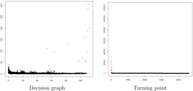
γ_ig = δg_i.ρg_i are computed, sorted and the turning-point-based decision rule from [11] presented in related work is applied to obtain the cluster centers. The selected centroids take each an unique label and the remaining balls receive the same label than their NHPD. Finally, each data point are labelled as the closest terminal ball containing it.

The complete procedure of IDPC is summarized in Algorithm 7.

Algorithm 5 Champions election

1: procedure _ChampElect(Ftree, {ρkg}g,k,{Bgk}g,k)

2: for g ∈ {G−1, ...,1} do

3: for all B_lg do

4: if B_lg is terminal then

5: ρg_champ,l(B_lg)←ρg_l(Bg_l)

6: cg_l ←G−g . Upgrade champions level

7: else 8: B_jg+1 ←argmax_Bg+1 i ∈D(B g l)(ρ g+1 champ,i(B g+1 i )) 9: ρg_champ,l(B_lg)←ρg+1_champ,j(B_jg+1) 10: cg+1_j ←G−g 11: end if 12: end for 13: end for 14: return ({ρg_champ,k}g,k,{c g k}k,g) 15: end procedure

5

Experimental results

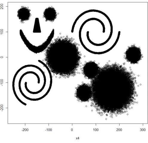
The generated dataset is composed by 1024508 bidimensional points in the rectangular domain [−300,300]×[−300,300]. It contains 13 clusters, its distribution can be seen in the figure 1. The ICMDW has been applied with Nmin = 0.1%N and R = 3₄.

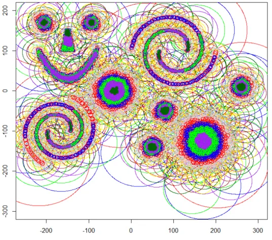
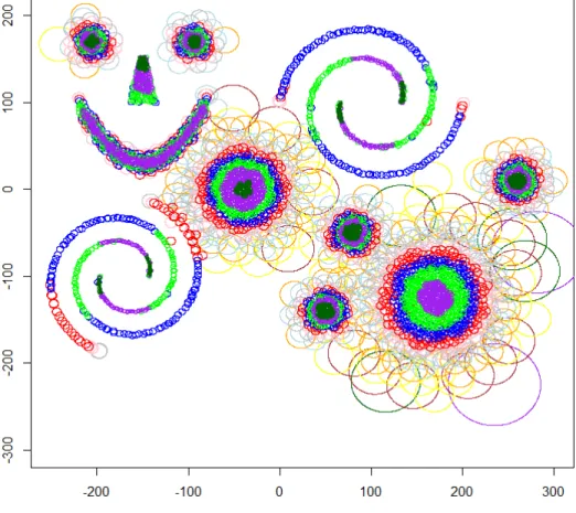
It produced a set of 9224 balls (figure 2), including the 4622 terminal balls (figure 3), all generations confounded. The total number of generations was 16.

Algorithm 6 Tree-dive

procedure _Tree-Dive(B,Ftree, c,{ρ

g

champ,k}g,k)

T ←F alse

Load BM .mother of the ball that promoted B to level c

while T ==F alse do Load s←D(BM) . daughters of BM sc +← {Bic|ρcchamp,i(Bic)> ρ(B)} j ←argmin_i(distance(B, s+[i])) if Bc

j is a terminal Ball then

T ←T rue else BM ←Bjc c←c+ 1 end if end while nhpd ←Bc j δ ←distance(B, B_jc) return {δ,nhpd} end procedure

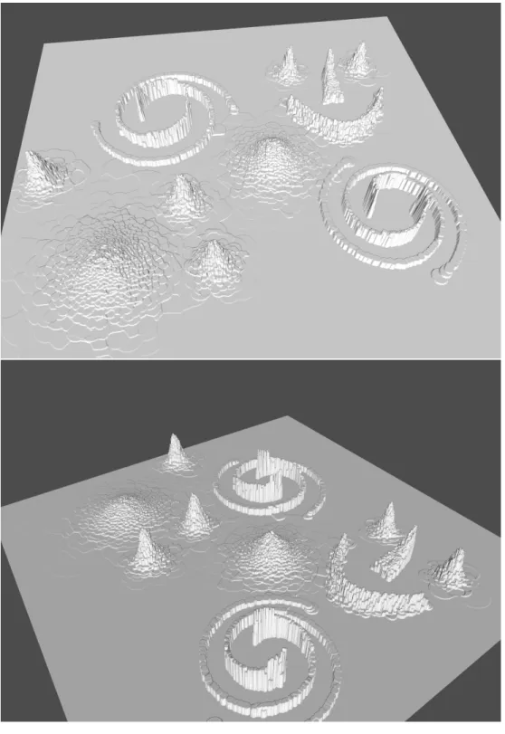
The density map is represented in the figure 4 over two different points of view. To construct this graphic we have created a grid of points covering the domain and associated, for each point of the grid, the density of the closest terminal ball containing it, to finally plot the surface. The density is well represented however there is some moderatly dense balls wich are supposed to carry a null or very low density. This problem that we call aliasing occurs in low density areas located near an abrupt peak. An aliasing ball is a ball that has been created lately (at a given generation), preventing it to increase its density count with the points that have been drawn before its creation. Therefore it is set terminal and get back its density at the density reevaluation phase. Even if the density map doesn’t reflect perfectly the true density, the aliasing can only create relatively low density balls (because of the large width of the window dg

c) near a much higher density peak. So its impact on clustering is almost inexistent.

The cluster centers can now be selected. We can see in the decision graph (figure 5) 13 points standing out the others. They are automatically detected with the turning-point

Algorithm 7 IDPC procedure _IDPC Nmin ←0.1%N d1_c ←1 Pseudo Normalize Randomize {{B_kg}g,k, Ftree,{ρ g k}g,k,{T Bg}g,{cci}i} ←ICM DW(d1c, Nmin, R) {{ρg_champ,k}g,k,{cg_k}k,g} ←CHAMPELECT(Ftree,{B_kg}g,k,{ρg_k}g,k)

for all (g, k)do {δ_kg,nhpd_g,k} ←TREE-DIVE(B_kg, Ftree, c g k,{ρ g champ,k}g,k) end for γ ←sort(δ.ρ) for i← {1, ..., m} do k1 i ← γi−γ1 i−1 ki₁−1 ← γi+1−γi 1 end for tp←argmax_i∈{1,...,m}( k1 i ki−1 1 ) .Turning-point for all j ≤tp do Label[j]←j end for

for all j ≥tp+ 1 do . Labelise Balls

Label[j]←Label[nhpd_j]

end for

for i← {1, ..., N} do . Labelise datapoints

Label[i]←Label[cci]

end for return Label

end procedure

procedure. The sorted gamma values are represented in the figure 5 and the selected cluster centers are represented in red and their location and the corresponding clustering results obtained by propagation of the label are showed in the figure 6.

Note that we didn’t have generated any flat clusters (like an uniform) because the original algorithm, and so our, isn’t able to deal with. In those situations, the algorithm may detect several peaks for only one real cluster. In a future work, we will benefit from the reduced set of pretender centroids and their localisation information provided by our algorithm to develop a better cluster center selection. To do so we might not only take into account the distance separating two peaks but rather the density connectivity between them. In other

Figure 1. Generated dataset

Decision graph Turning point

Figure 5. Center selection

Cluster centers Labelled dataset

6

Conclusion and future work

Many extensions of FDPC have been developed but none is able to deal with multidimen-sional and large datasets that arise in many pratical data analysis applications. In this paper we have presented an efficient algorithm able to manage those kind of data.

For that purpose, we have designed an iterative procedure which creates both localisa-tion and density map which gives, in a computalocalisa-tionaly efficient way, the densities ρi and the distances δi.

It is adaptive, the results being barely influenced by the few free parameters to be tuned, so that the automatic choice is often satisfactory. This last point is a dramatic improvement over most of the existing algorithms that tend to depend critically on the initial conditions.

An important remaining work to be performed is the recoding of the procedure in a compiled language with optimized data structures, from which a gain of at least an order of magnitude is expected. Moreover we aim to develop a better cluster selection unlocked by our intermediate results, able to manage flat distributions. Finally, we expect to delete the aliasing in the density map.

References

[1] Dongxia Chang, Yao Zhao, Lian Liu, and Changwen Zheng. A dynamic niching clus-tering algorithm based on individual-connectedness and its application to color image segmentation. Pattern Recognition, 2016.

[2] Zhensong Chen, Zhiquan Qi, Fan Meng, Limeng Cui, and Yong Shi. Image segmenta-tion via improving clustering algorithms with density and distance. Procedia Computer Science, 55:1015–1022, 2015.

[3] Yizong Cheng. Mean shift, mode seeking, and clustering. IEEE Transactions on Pattern Analysis and Machine Intelligence, 1995.

[4] Haizhou Du et al. Robust local outlier detection. In 2015 IEEE International Con-ference on Data Mining Workshop (ICDMW), pages 116–123. IEEE, 2015.

[5] Martin Ester, Hans-Peter Kriegel, Jörg Sander, Xiaowei Xu, et al. A density-based algorithm for discovering clusters in large spatial databases with noise. In Kdd, vol-ume 96, pages 226–231, 1996.

[6] Sen Jia, Guihua Tang, and Jie Hu. Band selection of hyperspectral imagery using a weighted fast density peak-based clustering approach. In International Conference on Intelligent Science and Big Data Engineering, pages 50–59. Springer, 2015.

[7] Shuai Li, Xiaofeng Zhou, Haibo Shi, and Zeyu Zheng. An efficient clustering method for medical data applications. In Cyber Technology in Automation, Control, and In-telligent Systems (CYBER), 2015 IEEE International Conference on, pages 133–138. IEEE, 2015.

[8] Zhou Liang and Pei Chen. Delta-density based clustering with a divide-and-conquer strategy: 3dc clustering. Pattern Recognition Letters, 73:52–59, 2016.

[9] Dongchang Liu, Shih-Fen Cheng, and Yiping Yang. Density peaks clustering approach for discovering demand hot spots in city-scale taxi fleet dataset. In2015 IEEE 18th In-ternational Conference on Intelligent Transportation Systems, pages 1831–1836. IEEE, 2015.

[10] Peiyu Liu, Yingying Liu, Xiuyan Hou, Qingqing Li, and Zhenfang Zhu. A text clus-tering algorithm based on find of density peaks. In 2015 7th International Conference on Information Technology in Medicine and Education (ITME), pages 348–352. IEEE, 2015.

[11] Chun-lai Ma, Tao Ma, and Hong Shan. A new important-place identification method. In Computer and Communications (ICCC), 2015 IEEE International Conference on, pages 151–155. IEEE, 2015.

[12] James MacQueen et al. Some methods for classification and analysis of multivariate observations. InProceedings of the fifth Berkeley symposium on mathematical statistics and probability, volume 1, pages 281–297. Oakland, CA, USA., 1967.

[13] Rashid Mehmood, Rongfang Bie, Hussain Dawood, and Haseeb Ahmad. Fuzzy clus-tering by fast search and find of density peaks. In 2015 International Conference on Identification, Information, and Knowledge in the Internet of Things (IIKI), pages 258–261. IEEE, 2015.

[14] Rashid Mehmood, Guangzhi Zhang, Rongfang Bie, Hassan Dawood, and Haseeb Ah-mad. Clustering by fast search and find of density peaks via heat diffusion. Neuro-computing, 2016.

[15] Li Miao. Comparative analysis of two clustering algorithms: K-means and fsdp (fast search and find of density peaks). 2015.

[16] Yan Qin, Chunhui Zhao, and Furong Gao. An iterative two-step sequential phase partition (itspp) method for batch process modeling and online monitoring. AIChE Journal, 62(7):2358–2373, 2016.

[17] Alex Rodriguez and Alessandro Laio. Clustering by fast search and find of density peaks. Science, 344(6191):1492–1496, 2014.

[18] Yong Shi, Zhensong Chen, Zhiquan Qi, Fan Meng, and Limeng Cui. A novel clustering-based image segmentation via density peaks algorithm with mid-level feature. Neural Computing and Applications, pages 1–11.

[19] Guangtao Wang and Qinbao Song. Automatic clustering via outward statistical testing on density metrics.

[20] Shuliang Wang, Dakui Wang, Caoyuan Li, Yan Li, and Gangyi Ding. Clustering by fast search and find of density peaks with data field. Chinese Journal of Electronics, 25(3):397–402, 2016.

[21] Xiao-Feng Wang and Yifan Xu. Fast clustering using adaptive density peak detection.

Statistical methods in medical research, page 0962280215609948, 2015.

[22] Yi Wang, Qixin Chen, Chongqing Kang, and Qing Xia. Clustering of electricity con-sumption behavior dynamics toward big data applications.

[23] Zhang WenKai and Li Jing. Extended fast search clustering algorithm: Widely density clusters, no density peaks.

[24] Juanying Xie, Hongchao Gao, Weixin Xie, Xiaohui Liu, and Philip W Grant. Robust clustering by detecting density peaks and assigning points based on fuzzy weighted k-nearest neighbors. Information Sciences, 354:19–40, 2016.

[25] Jia Yu, Lei Xie, Xiong Xiao, Eng Siong Chng, and Haizhou Li. A density peak clustering approach to unsupervised acoustic subword units discovery. In 2015 Asia-Pacific Signal and Information Processing Association Annual Summit and Conference (APSIPA), pages 178–183. IEEE, 2015.

[26] Ruisheng Zhang, Huiyi Ma, Qidong Liu, and Zhili Zhao. An improved fast search clustering algorithm based on kernel density. In 2015 IEEE International Conference on Smart City/SocialCom/SustainCom (SmartCity), pages 689–693. IEEE, 2015.