Random Neural Networks and Optimisation
Stelios Timotheou
A thesis submitted for the degree of
Doctor of Philosophy of Imperial College London
Department of Electrical and Electronic Engineering
Imperial College London
United Kingdom
I dedicate this thesis to my father, Andreas Timotheou,
who passed away on the 26th October 2007, after a stoical battle with cancer. May God rest his soul.
Abstract
In this thesis we introduce new models and learning algorithms for the Random Neural Network (RNN), and we develop RNN-based and other approaches for the solution of emergency management optimisation problems.
With respect to RNN developments, two novel supervised learning algorithms are proposed. The first, is a gradient descent algorithm for an RNN extension model that we have introduced, the RNN with synchronised interactions (RNNSI), which was inspired from the synchronised firing activity observed in brain neural circuits. The second algorithm is based on modelling the signal-flow equations in RNN as a nonnegative least squares (NNLS) problem. NNLS is solved using a limited-memory quasi-Newton algorithm specifically designed for the RNN case.
Regarding the investigation of emergency management optimisation problems, we examine combinatorial assignment problems that require fast, distributed and close to optimal solution, under information uncertainty. We consider three dif-ferent problems with the above characteristics associated with the assignment of emergency units to incidents with injured civilians (AEUI), the assignment of as-sets to tasks under execution uncertainty (ATAU), and the deployment of a robotic network to establish communication with trapped civilians (DRNCTC).
AEUI is solved by training an RNN tool with instances of the optimisation prob-lem and then using the trained RNN for decision making; training is achieved using the developed learning algorithms. For the solution of ATAU problem, we intro-duce two different approaches. The first is based on mapping parameters of the optimisation problem to RNN parameters, and the second on solving a sequence of minimum cost flow problems on appropriately constructed networks with estimated arc costs. For the exact solution of DRNCTC problem, we develop a mixed-integer linear programming formulation, which is based on network flows. Finally, we de-sign and implement distributed heuristic algorithms for the deployment of robots when the civilian locations are known or uncertain.
Acknowledgements
First and foremost I would like to thank my supervisor, Professor Erol Gelenbe, for his constant support, not only academically and financially, but also on a personal level. I deeply appreciate his persistent care and efforts to address my needs and problems, and I am grateful for the opportunities he provided me to travel and interact with members of the academia and industry worldwide. His expertise and guidance proved invaluable during my first steps as a junior researcher. He will always be an inspirational figure to me.
I am also thankful to my family for their encouragement throughout this demand-ing period of my life, and especially my wife Maria. If she had not unconditionally offered her love, patience, and support in every possible way to keep me focussed, often at the expense of her own work, this thesis would have been unattainable.
Moreover I would like to thank my colleagues at the Intelligent Systems & Net-works Group, who created a sincerely supportive working environment. Special acknowledgements go to George, Avgoustinos, and Georgia, for eagerly sharing their knowledge and time whenever I asked them. Also, I would like to express my gratitude to all my good friends, and particularly Evelina for her insights into com-binatorial optimisation, and Yannis for his heartening support and spot-on advice on any concern I confided to him.
Finally, I would like to acknowledge the Cyprus State Scholarships Foundation and the ALADDIN (Autonomous Learning Agents for Decentralised Data and In-formation Networks) project, for funding my studies.
Contents
List of Figures 10
List of Tables 13
Abbreviations and Acronyms 14
List of main symbols 16
List of Author Publications 20
1. Introduction 23
1.1. Application context: disaster management . . . 24
1.2. Review of examined problems . . . 25
1.3. Summary of contributions . . . 26
1.4. Thesis outline . . . 28
2. The random neural network 31 2.1. Introduction . . . 31
2.2. The random neural network model . . . 32
2.2.1. Mathematical model . . . 32
2.2.2. Network behaviour in steady-state . . . 33
2.2.3. Network Stability . . . 35
2.2.4. Analogy with the formal neural networks . . . 36
2.2.5. Function approximation . . . 37
2.2.6. Hardware implementations . . . 38
2.3. RNN extension models . . . 38
2.3.1. Bipolar random neural network . . . 39
2.3.2. RNN with state-dependent firing . . . 39
2.4. Learning algorithms . . . 40
2.4.1. Gradient descent supervised learning algorithm for the RNN model . . . 41
2.4.2. Alternative RNN supervised learning algorithms . . . 44
2.4.3. Reinforcement learning in RNN . . . 45
2.5. Applications . . . 48
2.5.1. Solution of optimisation problems . . . 48
2.5.2. Modelling applications . . . 52
2.5.3. Learning applications . . . 53
2.6. Conclusions . . . 54
3. Learning extensions of the random neural network model 56 3.1. Introduction . . . 57
3.2. Gradient descent learning in the RNN with synchronised interactions 60 3.2.1. Synchronised interactions in biological neural networks . . . 60
3.2.2. RNNSI mathematical model . . . 61
3.2.3. Steady-state solution . . . 62
3.2.4. RNNSI gradient descent supervised learning . . . 64
3.2.5. Computational complexity . . . 67
3.3. RNN supervised learning using nonnegative least squares . . . 71
3.3.1. Problem formulation . . . 72
3.3.2. Solution approach . . . 75
3.3.3. Efficient computation of NNLS costly functions . . . 88
3.3.4. Computational complexity . . . 96
3.4. Conclusions . . . 98
4. Assignment of emergency units to incidents 100 4.1. Problem description . . . 101
4.2. Supervised learning solution approach . . . 103
4.3. Performance evaluation of the RNNSI learning algorithm . . . 105
4.4. Performance evaluation of the RNN-NNLS algorithm . . . 112
4.4.1. Preliminary results . . . 113
4.4.2. Solving the AEUI problem . . . 116
4.5. Using RNN-NNLS algorithm for weight initialisation . . . 121
5. Asset-task assignment under execution uncertainty 127
5.1. Introduction . . . 128
5.2. Problem description and mathematical formulation . . . 130
5.3. Related problems . . . 131
5.4. The RNN parameter association approach . . . 134
5.5. Network flow algorithms . . . 137
5.6. Obtaining tight lower bounds . . . 142
5.7. Evaluation . . . 147
5.8. Conclusions . . . 153
6. Connecting trapped civilians to a wireless ad-hoc robotic network154 6.1. Introduction . . . 155
6.2. Related work . . . 157
6.3. Assumptions . . . 157
6.4. A centralised approach . . . 158
6.4.1. Formulation . . . 158
6.4.2. Numerical results using the general centralised approach . . 161
6.4.3. Numerical results for uncertain civilian locations . . . 162
6.4.4. Minimising the number of robots and the energy consumption 164 6.5. A distributed heuristic . . . 167
6.5.1. Simulation results for the distributed algorithm . . . 170
6.5.2. Introducing uncertainty . . . 171
6.5.3. MST-based modification . . . 174
6.6. Conclusions . . . 177
7. Conclusions and future work 178 7.1. Thesis contributions . . . 178
7.2. Future work . . . 182
Bibliography 185
Appendices 204
B. Derivation of expressions associated with the efficient computation
of NNLS costly functions 208
B.1. The first approach . . . 208
B.1.1. Derivation of Eq. (3.60) . . . 208
B.1.2. Derivation of Eq. (3.64) . . . 209
B.2. The second approach . . . 210
B.2.1. Derivation of Γlm . . . 211
List of Figures
4.1. Dispatching of emergency units to locations of injured civilians . . . 101 4.2. Performance of the RNNSI gradient descent algorithm for the
“col-lective” neural network architecture . . . 107 4.3. Performance of the RNN gradient descent algorithm for the
“collec-tive” neural network architecture . . . 108 4.4. Performance of the RNNSI gradient descent algorithm for the
“indi-vidual” neural network architecture . . . 109 4.5. Performance of the RNN gradient descent algorithm for the
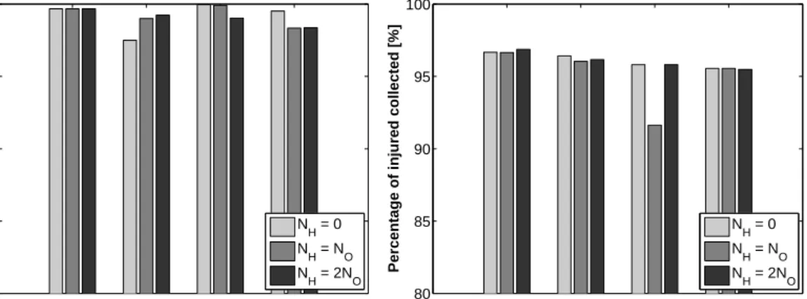
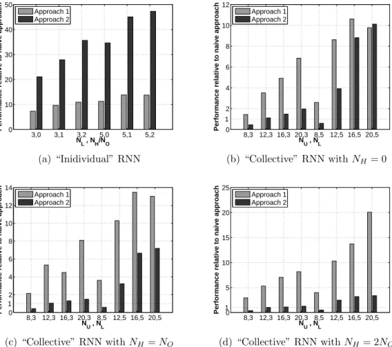
“indi-vidual” neural network architecture . . . 110 4.6. Performance evaluation of the four architectures considered: (a)
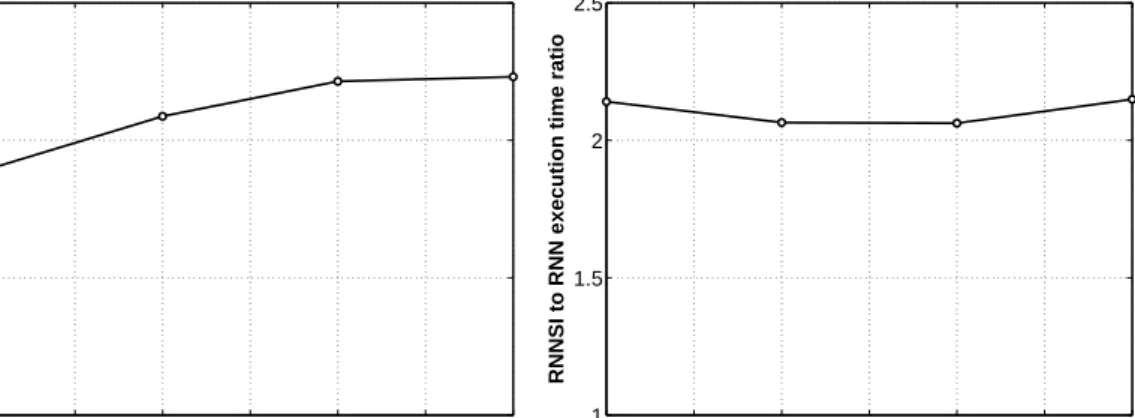
“Col-lective” RNNSI , (b) “Col“Col-lective” RNN, (c) “Individual” RNNSI, and (d) “Individual” RNN . . . 111 4.7. RNNSI to RNN execution time ratio . . . 113 4.8. Performance of approaches for computing the objective and gradient
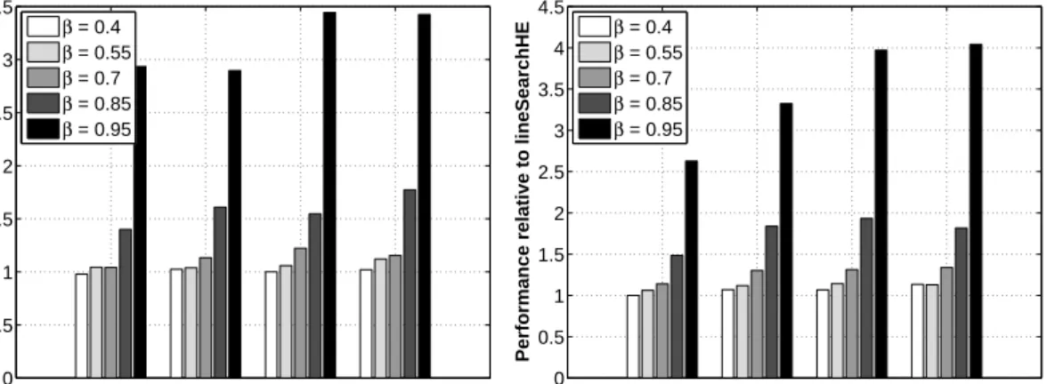
NNLS function compared to a “naive” one; the metric used is the ratio of execution times between the naive and another approach . . 114 4.9. Comparison of line search procedures lineSearchLin and lineSearchHE
in terms of matrix vector products (the y-axis is their ratio) for
NL = 3 andNL = 5 when NH =NO . . . 115
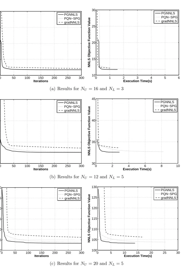
4.10. Comparison of convergence between algorithms gradNNLS, PQN-SPG and PGNNLS with respect to iterations and execution time . . 117 4.11. Convergence of RNN-NNLS algorithm for NL= 3 and NL= 5 when
NH = 2NO . . . 118
4.12. Performance of the NNLS-RNN algorithm for the “collective” neural network architecture . . . 119 4.13. Performance of the NNLS-RNN algorithm for the “individual” neural
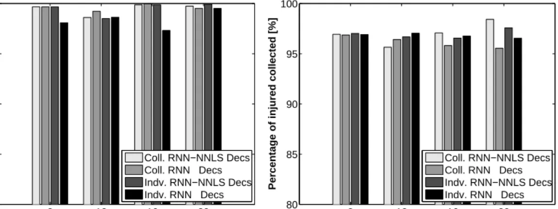
4.14. Comparison between the RNN-NNLS and RNN learning algorithms. The four architectures considered are: (a) “Collective” RNN-NNLS, (b) “Collective” RNN, (c) “Individual” RNN-NNLS, and (d) “Indi-vidual” RNN . . . 122 4.15. Performance of the RNN learning algorithm with random or NNLS
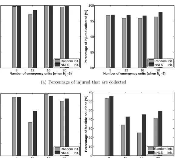
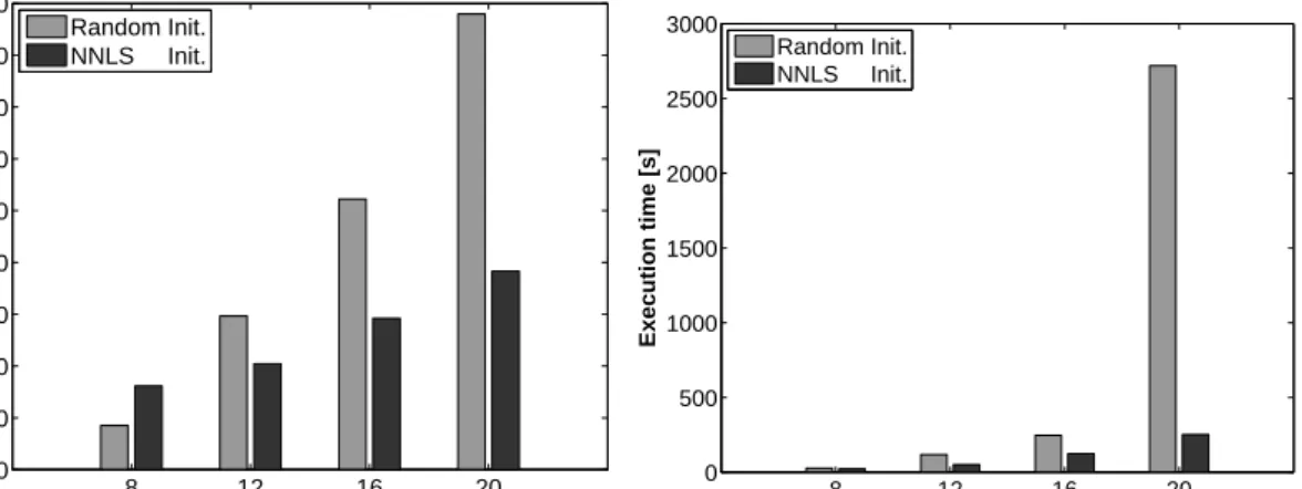
initialisation for the “collective” NN architecture, with no hidden neurons. . . 124 4.16. Execution times of the RNN learning algorithm with random or
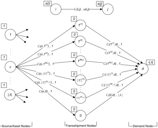
NNLS initialisation . . . 125 5.1. Flow network for the solution of problem (5.2) . . . 137 5.2. Piecewise linear approximation . . . 145 6.1. Example scenario: A group of robots establish communication with
trapped civilians . . . 156 6.2. Robot allocations according to the centralised solutions for (i)Rrob =
8m and Rciv = 4m, (ii)Rrob = 14m and Rciv = 4m, (iii)Rrob = 8m
and Rciv = 14m: When the civilian range is small one robot must be
dedicated to each civilian, whereas when it is large one robot may suffice to connect multiple civilians. In addition, when the robot range is not large enough, a significant number of the robots must be used for maintaining connectivity; hence, they move to locations of high density of civilians for optimal performance. . . 163 6.3. Maximum number of connected civilians for varying Rciv and Rrob =
8m,10m,12m . . . 164 6.4. Maximum number of connected civilians for varying Rrob andRciv =
2m,6m,10m . . . 165 6.5. Maximum number of connected civilians for varying number of robots
and different combinations of ranges . . . 166 6.6. Average percentage of connected civilians for varyingRrobandRciv =
2m,6m,10m, for uncertain civilian locations . . . 167 6.7. Average percentage of connected civilians for varying number of
robots, for uncertain civilian locations . . . 168 6.8. Minimum number of robots required to connect all civilians when
6.9. Average locomotion energy consumed per robot when objectives (6.2a), (6.5) and (6.6) are utilised. . . 169 6.10. General flow diagram of the distributed heuristic algorithm . . . 169 6.11. Solution of the distributed algorithm for the given clustering of civilians171 6.12. Comparison between the distributed and centralised approach in
terms of number of connected civilians against the number of robots 172 6.13. Comparison between the distributed and centralised approach in
terms of number of connected civilians against the wireless range of the robots . . . 172 6.14. Connectivity is guaranteed within a cluster if its radius is smaller
than Rrob+Rciv . . . 173
6.15. Evaluation of the distributed heuristic for different numbers of robots
Nrob and varying risk parameter q . . . 174
6.16. Illustration of the Minimum Spanning Tree formed by the clusters and the movement options of the robots . . . 175 6.17. Percentage of trapped civilians connected against time for 10, 15 and
List of Tables
2.1. Summary of RNN applications . . . 55 4.1. Optimal regularisation weights for the “collective” RNN architecture 121 5.1. Average relative percentage deviation from the optimal solutions of
data family 1 . . . 147 5.2. Average relative percentage deviation from the optimal solutions of
data family 2 . . . 148 5.3. Average relative percentage deviation from the lower bound of data
family 1 . . . 150 5.4. Average relative percentage deviation from the lower bound of data
Abbreviations and Acronyms
AEUI Assignment of Emergency Units to Incidents ANN Artificial Neural Networks
APA Armijo along the Projection Arc
ATAU Asset-Task Assignment under execution Uncertainty BFGS Broyden - Fletcher - Goldfarb - Shanno
BRNN Bipolar Random Neural Network CPN Cognitive Packet Network
CRNN Clamped Random Neural Network DFP Davidon - Fletcher - Powell
DRNCTC Deployment of a Robotic Network for Communication with Trapped Civilians
DRNN Dynamic Random Neural Network ES Expected Shortfall
FNNLS Fast NonNegative Least Squares KKT Karush-Kuhn-Tucker
LBA Lower Bounding Algorithm MCF Minimum Cost Flow
MCRNN Multiple Class Random Neural Network MMR Maximum Marginal Return
MSE Mean Square Error MST Minimum Spanning Tree
MSTP Minimum Steiner Tree Problem MVCP Minimum Vertex Covering Problem NN Neural Network
NNLS NonNegative Least Squares
NP-hard Non-determenistic Polynomial-time hard
PGNNLS Projected Gradient NonNegative Least Squares PQN Projected Quasi Newton
QoS Quality of Service
QSAP Quadratic Semi-Assignment Problem RL Reinforcement Learning
RNN Random Neural Network
RNNSDF Random Neural Network with State-Dependent Firing RNNSI Random Neural Network with Synchronised Interactions RPROP Resilient Propagation
SATP Satisfiability Problem SF Synchronised Firing
SPG Spectral Projected Gradient WTA Weapon Target Assignment
List of main symbols
RNN and RNNSI symbols
ki(t) Potential of neuron iat time t
qi(t) Probability neuroni is excited at time t
Λi External arrival rate of positive signals to neuron i λi External arrival rate of negative signals to neuron i λ+(i) Total arrival rate of positive signals to neuroni
λ−(i) Total arrival rate of negative signals to neuroni
p+(i, j) Probability neuronj receives a positive signal from firing neuron i
p−(i, j) Probability neuronj receives a negative signal from firing neuroni
Q(i, j, l) Probability of firing neuron i to create a synchronous interaction
together with neuronj to affect neuron l
w+(i, j) Rate of positive signals or positive weight to neuron j from firing neuroni
w−(i, j) Rate of negative signals or negative weight to neuronj from firing neuroni
w(i, j, l) Rate or weight of synchronous interactions to neuron l generated
from firing neuron itogether with neuron j a(j, l) Ratio of w(i, j, l) over w−(i, j)
W+ Matrix of positive weights
W− Matrix of negative weights
A Matrix of parametersa(j, l)
d(i) Probability a signal from firing neuron i departs from the network
ri Firing rate of neuron i
N Number of neurons in the network
N(i) Nominator of the equation describing the excitation probability of neuroni
D(i) Denominator of the equation describing the excitation probability of neuroni
xik The ith input value of the kth training pair
yik The ith output value of thekth training pair Iout Set of output neurons
Iout Set of non-output neurons
NNLS-related symbols
B Matrix of the NNLS formulation
b Vector of the NNLS formulation
w Decision variables of the NNLS formulation
τ Represents the τth iteration of the algorithm
F Free-set of variables
B Binding-set of variables
S Gradient scaling matrix
d Search-direction
θ1 Weight for l1-norm regularisation
θ2 Weight for l2-norm regularisation
∆g Change of gradient vector between successive iterations ∆w Change of decision vector between successive iterations
M Number of correction vectors for limited-memory BFGS update
Symbols of AEUI problem
NU Number of emergency units NL Number of incident locations
Tij Response time of emergency unit ito incident j Ij Number of people injured at incident j
Symbols of ATAU problem
A Set of assets
T Set of tasks
U(t) Cost of task t
Ca(a, t) Cost of assigning asset a to task t
ps(a, t) Probability that asset a will succeed in executing task t pf(a, t) Probability that asset a will fail in executing task t
max{0, b(a, t)} Net expected reduction in the objective function for (a, t) assign-ment pair
at(m) Asset a is the mth assignment to task t
Symbols of DRNCTC problem
R Set of robots
C Set of civilians
Rrob Connectivity range of robots Rciv Connectivity range of civilians
yc Decision variable indicating whether civilian cis connected xi Decision variable showing whether there is a robot at vertex i
CRR
i,j Element of matrix CRR representing whether a robot on vertex j
would be connected with a robot on vertexi
CRC
c,j Element of matrix CRC representing whether a robot on vertex j
would be connected to civilianc
Ci,jRL Element of matrix CRL representing whether a robot at location i
can connect civilians at location j
Ei,j Energy consumed by a robot to move from nodei toj E[Zi] Expected number of civilians on vertexi
Symbols of MCF problem
N Set of nodes or vertices
E Set of arcs or edges
Xf(i, j) Decision variable representing the flow on arc (i, j) Cf(i, j) Cost per unit of flow on arc (i, j)
u(i, j) Flow capacity of arc (i, j)
d Demand or sink node
List of Author Publications
Journal Papers
J1. Timotheou, S. (2011) Asset-task assignment algorithms in the presence of exe-cution uncertainty, The Computer Journal, accepted for publication: Oxford University Press. [Special issue of ISCIS’10]
J2. Gelenbe, E., Timotheou, S. and Nicholson, D. (2010) Fast Distributed Near-optimum Assignment of Assets to Tasks, The Computer Journal, Advance Access published on February 19, 2010, 10.1093/comjnl/bxq010.
J3. Timotheou, S. (2010) The Random Neural Network: A Survey, The Computer Journal, 53(3), 251-267: Oxford University Press.
J4. Timotheou, S. (2009) A Novel Weight Initialization Method for the Random Neural Network, Neurocomputing, 73(2), 160-168: Elsevier. [Special issue of ISNN’08]
J5. Gelenbe, E. and Timotheou, S. (2008) Random Neural Networks with Synchro-nized Interactions, Neural Computation, 20(9), 2308-2324: MIT Press.
J6. Gelenbe, E. and Timotheou, S. (2008) Synchronized Interactions in Spiked Neuronal Networks, The Computer Journal, 51(6), 723-730: Oxford Univer-sity Press.
Conference Papers
C1. Timotheou, S. (2010) Network flow approaches for an asset-task assignment problem with execution uncertainty, To appear in Proceedings of the 25th In-ternational Symposium on Computer and Information Sciences (ISCIS’10),
London, United Kingdom, 22-24 September, Lecture Notes in Electrical En-gineering: Springer, Berlin / Heidelberg. [Extended version to appear in special issue of The Computer Journal]
C2. Gelenbe, E., Timotheou, S. and Nicholson, D. (2010) A Random Neural Net-work Approach to an Assets to Tasks Assignment Problem, InProceedings of SPIE Symposium on Defense, Security and Sensing, 7697(76970Q), Orlando, Florida, 5-9 April. SPIE, Bellingham, WA.
C3. Gelenbe, E., Timotheou, S. and Nicholson, D. (2010) Random Neural Net-work for Emergency Management, n Proceedings of the Workshop on Grand Challenges in Modeling, Simulation, and Analysis for Homeland Security (MSAHS’10), Washington, D.C., 17-18 March. Directorate of Science & Tech-nology, US Department of Homeland Security, Washington, D.C.
C4. Filippoupolitis, A., Loukas, G., Timotheou, S., Dimakis, N. and Gelenbe, E. (2009) Emergency Response Systems for Disaster Management in Buildings, In Proceedings of NATO IST-086 Symposium on C3I for Crisis, Emergency and Consequence Management, Bucharest, Romania, 1112 May, pp. 151 -15-14. NATO-RTO [Best Paper Award].
C5. Timotheou, S. and Loukas, G. (2009), Autonomous Networked Robots for the Establishment of Wireless Communication in Uncertain Emergency Response Scenarios, 24th ACM Symposium on Applied Computing (SAC’09), Honolulu, Hawaii, 8-12 March, pp. 1171-1175. ACM, NY.
C6. Loukas, G. and Timotheou, S. (2008) Connecting Trapped Civilians to a Wire-less Ad Hoc Network of Emergency Response Robots, In Proceedings of the 11th IEEE International Conference on Communication Systems (ICCS’08), Guangzhou, China, 19-21 November, pp. 599-603. IEEE, Piscataway, NJ.
C7. Loukas, G., Timotheou, S. and Gelenbe, E. (2008) Robotic Wireless Network Connection of Civilians for Emergency Response Operations, In Proceedings of the 23rd International Symposium on Computer and Information Sciences (ISCIS’08), Istanbul, Turkey, 27-29 October, pp. 1-6. IEEE, Piscataway, NJ.
C8. Timotheou, S. (2008) A Novel Weight Initialization Method for the Random Neural Network,5th International Symposium on Neural Networks (ISNN’08),
Beijing, China, 24-28 September. [Appears in special issue of Neurocomput-ing, 73(2), 160-168: Elsevier].
C9. Timotheou, S. (2008) Nonnegative Least Squares Learning for the Random Neural Network, In Proceedings of the 18th International Conference on Arti-ficial Neural Networks (ICANN’08), Prague, Czech Republic, 3-6 September 2008, Lecture Notes Computer Science, Part I, 5163, pp. 195-204: Springer, Berlin / Heidelberg.
C10. Filippoupolitis, A., Gelenbe, E., Gianni, D., Hey, L., Loukas, G. and Tim-otheou, S. (2008) Distributed Agent-oriented Building Evacuation Simula-tor, In Proceedings of the 2008 Summer Computer Simulation Conference (SCSC’08), Edinburgh, Scotland, 16-19 June. SCS, Vista, CA.
C11. Filippoupolitis, A. Hey, L., Loukas, G., Gelenbe, E. and Timotheou, S. (2008) Wireless Sensor Networks in Augmented Reality: Emergency Response Sim-ulation, InProceedings of the 1st International Conference on Ambient Media and Systems (Ambi-Sys’08), Quebec City, Canada, 11-14 February, pp. 1-7. ICST, Brussels, Belgium.
Poster Presentations
P1. Timotheou, S. and Gelenbe, E. (2009) Random Neural Networks with Synchro-nized Interactions, 2nd Symposium of the Neuroscience Technology Network, London, United Kingdom, 7 October 2009.
P2. Gelenbe, E. and Timotheou, S. (2008) Spiked Random Neural Networks with Synchronized Firing, Symposium on Perspectives in Modeling and Perfor-mance Analysis of Computer Systems & Networks (Model35), Paris-Rocquencourt, France, 2-3 April 2008.
P3. Filippoupolitis, A., Gelenbe, E., Gianni, D., Hey, L., Loukas, G. and Timoth-eou, S. (2008) A Distributed Multi-Agent Simulator for Building Evacuation,
Symposium on Perspectives in Modeling and Performance Analysis of Com-puter Systems & Networks (Model35), Paris-Rocquencourt, France, 2-3 April 2008.
1. Introduction
The main aim of this thesis is the investigation of different aspects of the Random Neural Network (RNN) and the development of corresponding algorithms for the solution of combinatorial optimisation problems. Specifically, we consider assign-ment problems which involve a number of agents, the decision makers, that need to act in order to optimise a common objective function subject to a number of global constraints. The examined problems have a number of challenging characteristics that should be addressed by any developed algorithms:
• Real-time solution: By “real-time” we mean that the time required by the optimisation algorithm to solve the problem is negligible compared to the time needed to execute any action imposed by the solution. For example, if the problem considered is the dispatching of ambulances to locations of accidents, then it is sufficient for the algorithm to provide a solution in milliseconds or a few seconds, since this time is negligible compared to the time that will be consumed by any of the ambulances to reach an accident. Hence, any developed algorithm should be fast and desirably of polynomial computational complexity to ensure that it will be executed in real-time for a given problem.
• Hard Problems: The considered problems are complex and of combinato-rial nature, resulting in NP-hard optimisation problems with exponentially increasing search spaces, which almost surely cannot be optimally solved with polynomial algorithms. As a result, the developed algorithms should provide close to optimal solutions despite being polynomial.
• Imperfect Information: In many cases, complete information about the problem dealt with cannot be collected, so that decision making has to rely on limited information. Limitations can occur in various forms, such as missing or imprecise data, ambiguity, or even uncertainty in the sense that we may only know the probability distribution rather than the actual value of particular
data. Hence, any developed algorithm should be able to appropriately handle these limitations by incorporating uncertainty into the model and utilising the available information in the best possible way.
• No central control: Having no central control is highly desirable for several reasons: (a) there is no central point of failure, (b) there is no communication bottleneck as there is no need to send all information to a central control unit, (c) local information can be incorporated into the decisions of individual agents.
1.1. Application context: disaster management
Problems with the aforementioned characteristics naturally arise in disaster or emergency management, which deals with physical and man-made incidents that threaten life, property, operations, or the environment. The process of disaster management involves four phases: (1) planning to reduce the effect or the risk of disasters (mitigation), (2) developing plans of actions to be used once a disaster occurs (preparedness), (3) responding to such situations (response) and (4) restor-ing the affected environments to their original state (recovery). The main goal of disaster management is to minimise the human casualties as well as the property and environmental damages in an emergency event [175, 142].Perhaps the most challenging of the four phases is the response phase, when the emergency services have to deal with the effects of the disaster in real-time, under extremely difficult conditions with imperfect information and usually dis-rupted communications. The following large-scale disaster scenario demonstrates a situation where optimisation problems with such characteristics arise:
A major earthquake has struck a large city during the morning hours of a week-day. As a result, several buildings have partially or fully collapsed and there are many injured civilians spatially distributed around the city. These civilians have to be found and collected by emergency units in the least possible time, taking into account the severity of their injuries, the limited number and capacity of the emergency units, as well as the fact that a number of roads have been blocked. Also a number of civilians have been trapped inside the ruins of the buildings so that search and rescue personnel need to identify their locations, assess their condition, and launch a rescue operation trying to maximise the number of collected civilians,
given that each one of them can only survive for a limited amount of time. In ad-dition, multiple fires have broken out around the city and need to be quickly dealt with by the fire-brigade taking into consideration the potential effect of each one of the fires, the weather conditions, and the scarcity of resources. To facilitate the rescue operations, the roads need to be unblocked starting from roads that accom-modate more traffic or that significantly increase the connectivity of the city. The work of the emergency services is further impaired by the fact that the communi-cation network has been disrupted, so that affected people cannot easily report to them incidents that require their attention. As the amount of information collected by the emergency services is limited, their actions need to also rely on a priori
known information. For example, if a number of buildings have collapsed, then the operations centre can take into consideration probability distributions associated with the number of people expected to be in each building, so as to prioritise their search and rescue operations.
The above scenario illustrates that in the event of a disaster, several complex optimisation problems with imperfect information may arise, requiring real-time and distributed decision making. In this thesis we will particularly look into three specific combinatorial optimisation problems of this nature, and develop algorithms for their solution mainly associated with the RNN. These problems are discussed in more detail in the next section.
1.2. Review of examined problems
In this thesis we will examine three different combinatorial problems that arise in emergency management:
1. Assignment of emergency units to incidents (AEUI): In this problem, a num-ber of incidents have taken place simultaneously and there are a numnum-ber of injured civilians at each location. At the time of the incidents, a number of emergency units are spatially distributed around the area, each having a different capacity to collect a number of those civilians, as well as a different response time to each of the incidents. The objective is to collect as many of the injured as possible and also minimise their total response time.
general problem associated with the assignment of assets to tasks when each asset can potentially execute any of the tasks, but assets execute tasks with a probabilistic outcome of success. There is a cost associated with each possible assignment of an asset to a task, and if a task is not executed there is also a cost associated with the non-execution of the task. Thus any assignment of assets to tasks will result in an expected overall cost which we wish to minimise. Assets can represent rescuers whose task is to collect a number of spatially distributed injured civilians. Each rescuer can collect at most one injured but it is uncertain whether s/he will be able to accomplish his/her task either because of difficulty in accessing the location of the injured or because s/he cannot handle the injured alone.
3. Deployment of a wireless ad hoc robotic network for the connection of trapped civilians (DRNCTC): During a disaster, emergency response operations can benefit from the establishment of a wireless ad hoc network. We investigate the use of autonomous robots that move inside a disaster area and estab-lish a network for two-way communication between trapped civilians with a priori known or uncertain locations and an operations centre. The civilians may have uncertain locations, in the sense that we only known a probability distribution describing the number of civilians at any possible position. The specific problem considered is to find optimal locations for the robots so that we maximise the number of civilians connected to the network, assuming that each civilian carries a short-range communication device. This problem is in close connection to the other two, as its solution can provide the means for locating and assessing the health condition of the injured civilians.
1.3. Summary of contributions
The contributions of this thesis can be divided into two main categories: (a) theoret-ical developments for the RNN and (b) mathemattheoret-ical formulation of the emergency management problems posed above and development of algorithms for their so-lution. The proposed algorithms are primarily based on RNN, but we have also developed network flow and greedy heuristic approaches. Specifically, the contribu-tions of this thesis are:
a. Theoretical developments for RNN
i. We have introduced RNNSI model, an extension of the RNN that incorpo-rates synchronous interactions and developed a gradient descent learning algorithm of the same computational complexity as the corresponding RNN algorithm.
ii. We have developed a new supervised learning algorithm for the RNN, called RNN-NNLS, that can be used both for learning and weight initialisation. The core of the algorithm is the solution of a nonnegative least squares (NNLS) problem formulated by approximating the RNN equations. So-lution to the NNLS problem is accomplished by a limited-memory quasi-Newton algorithm. We have also derived efficient analytical expressions for the computation of the objective and gradient NNLS functions, which speed up the procedure by up to fifty times.
iii. We have conducted the first extended survey on RNN, since its discovery two decades ago.
b. Investigation of emergency management optimisation problems
i. We have proposed a supervised learning methodology for the real-time solu-tion of hard combinatorial optimisasolu-tion problems when distributed and consistent decision making is necessary. In relation to that we have ex-amined the AEUI problem using the developed RNNSI and RNN-NNLS learning algorithms.
ii. For the solution of ATAU problem, we have developed an RNN param-eter association approach, in which the paramparam-eters of the optimisation problem are associated with parameters of the RNN model. In addition, we have proposed the use of network flow algorithms that are based on solving a sequence of minimum cost flow problems on appropriately con-structed networks with estimated arc costs and introduced three different estimation schemes. We have also designed an approach for obtaining tight lower bounds to the optimal solution based on a piecewise linear approximation of the considered problem.
iii. We have introduced the problem of maximising the number of connected trapped civilians to a wireless ad-hoc robotic network when the locations
of the civilians are either a priori known or uncertain. For its optimal solution, we have derived a mixed-integer linear programming formula-tion based on network flows. We have also designed and implemented distributed heuristic algorithms based on clustering possible locations of civilians both for certain and uncertain civilian locations.
1.4. Thesis outline
The remainder of this thesis is organised as follows. In Chapter 2 we survey the research work on the RNN, including the description and mathematical properties of the original model, other extensions that incorporate additional signal capabilities, RNN-related learning algorithms, as well as applications of the model with emphasis on those related to the solutions of combinatorial optimisation problems.
In Chapter 3, we present the developed RNNSI and RNN-NNLS learning al-gorithms. First, we describe the motivation for this work and discuss associated research. In the next section, we present the RNNSI learning algorithm. We start with a discussion of the model’s biological relevance and a description of its mathe-matical properties. Then, we derive the main steps of the algorithm; the details of the derivation are included in Appendix A. The section finishes with an extensive analysis of its computational complexity that results in efficient modifications of the algorithm. In the subsequent section, we discuss the details of the RNN-NNLS algorithm. Firstly, we illustrate how to obtain the NNLS formulation from the RNN supervised learning problem when all neurons have desired output values. Next, we develop a limited-memory quasi-Newton algorithm for the solution of the NNLS problem, and present the RNN-NNLS algorithm that can be employed for the solu-tion of problems involving both output and non-output neurons. Before discussing the computational complexity of RNN-NNLS, we outline two approaches for the efficient evaluation of the objective and gradient NNLS functions, by manipulating the special structure of the examined problem; the analysis of the corresponding expressions is given in Appendix B. The final section is a summary of the chapter’s outcomes.
The evaluation of the developed supervised learning algorithms is undertaken in Chapter 4, for the solution of the optimisation problem associated with the assign-ment of emergency units to incidents. We start with the description and
mathemat-ical formulation of the problem followed by the proposed solution approach, which is based on training a neural network tool to act as an “oracle” for decision making. For this purpose, the RNN and RNNSI models are employed and trained using the learning algorithms developed in Chapter 3. In the remainder of the chapter an extensive evaluation is carried out to show the learning ability of the proposed al-gorithms as well as their efficiency in solving the investigated problem. In addition to the performance evaluation of RNNSI and RNN-NNLS learning algorithms, we examine the efficiency of RNN-NNLS as a weight initialisation method and finish with the main conclusions of the chapter.
In Chapter 5, we examine the asset-task assignment problem under execution uncertainty. We start with the description and mathematical formulation of the problem, followed by a discussion of other related problems. Then, we describe two polynomial deterministic approaches for its solution: (a) an RNN algorithm based on associating parameters of the optimisation problem with parameters of RNN, and (b) a minimum cost flow algorithm that is based on estimating the cost values of specific arcs in the flow network. We also develop a piecewise linear approach for obtaining tight lower bounds to the studied problem, before examining the performance of the proposed approaches and concluding.
Chapter 6 studies the problem of deploying a wireless ad-hoc robotic network for the connection of trapped civilians. First, we discuss the motivation for the solution of this problem followed by a description of related research topics. Then, we give a formal description of the problem with the assumptions made and formulate it as a mixed-integer mathematical program that can be solved by a central processing unit. Apart from the centralised approach we also describe three versions of a dis-tributed heuristic algorithm for its solution. The first deals with the problem when the locations of the civilians are a priori known. The second is a modified version of the first one, which tackles the problem with uncertain civilian locations using a risk measure for economic theory, called expected shortfall. The third version is a modification of the second one, with which the deployment of robots relies on an appropriately constructedminimum spanning tree, aiming to reduce the connec-tion time of the civilians and the total energy spent by the robots. Performance evaluation of the developed algorithms in this section is undertaken throughout the chapter with respect to the centralised algorithm and between the different versions of the distributed heuristic.
Finally, in Chapter 7 we summarise the main contributions of this thesis and discuss possibilities for exploitation. The thesis finishes by providing directions for future work for the core research chapters.
2. The random neural network
This chapter attempts to briefly and comprehensively present the large amount of research published on the RNN since its introduction two decades ago. Our intention is to review the theory and present different RNN tools that can be utilised for the solution of practical problems.
The chapter is organised as follows: In section 2.1, an introduction on RNN is provided along with its main attractive features. The mathematical model and its steady-state properties are described in Section 2.2, while extension models are discussed in Section 2.3. Following is a presentation of the RNN learning algorithms, as well as algorithms proposed for RNN extension models. The RNN applications are summarised in Section 2.5, with particular emphasis on the approaches used for the solution of optimisation problems. The chapter concludes in section 2.6.
2.1. Introduction
The Random Neural Network (RNN) is a neural network model inspired by the spiking behaviour of biophysical neurons [56]. When a biophysical neuron is excited, it transmits a train of signals, called action potentials or spikes, along its axon to either excite or inhibit the receiving neurons. The combined effect of excitatory and inhibitory inputs changes the potential level of the receiving neuron and determines whether it will become excited. In RNN these signals are represented as excitatory and inhibitory spikes of amplitude +1 and -1 respectively, that are transmitted either from other neurons or from the outside world. Each neuron can fire only when its potential is strictly positive. The potential is equal to the number of positive spikes received that have not yet been fired or cancelled by inhibitory spikes.
RNN has attracted a lot of attention in the scientific community. Various aspects of it have been explored, while several extension models and learning algorithms
have been developed. In addition, RNN has found widespread application in di-verse areas of engineering and physical sciences. The success of the model can be attributed to its unique features which include the following [82]:
• Although it is a recurrent neural network, its steady-state probability distri-bution is described by an analytical equation that can be easily and efficiently computed without the use of Monte Carlo methods
• Its standard learning algorithm has low complexity and strong generalisation capacity even for a relatively small training data set
• It represents in a closer manner the signals transmitted in a biological neuronal network than other Artificial Neural Networks (ANN)
• It can be easily implemented in both software and hardware since its neurons can be represented by simple counters
• There is a direct analogy between the RNN and the connectionist ANN
• The neuron potential is represented as an integer rather than a binary variable resulting in a more detailed system-state description
• It is a universal approximator for bounded continuous functions
• The stochastic excitatory and inhibitory interactions in the network make it an excellent modelling tool for various interacting entities
2.2. The random neural network model
In this section, a mathematical description and the main results of the standard random neural network model are given. We also discuss the stability of the network as well as its analogy to connectionist ANN.
2.2.1. Mathematical model
RNN is a recurrent network ofN fully connected neurons which exchange positive and negative signals in the form of unit amplitude spikes. At any time t, the state of neuron i is described by its signal potential ki(t) which is a nonnegative integer
associated with the accumulation of positive signals at the neuron. We say that neuron i is excited when ki(t) > 0, else if ki(t) = 0 then it is idle or quiescent. A
closely related parameter isqi(t) = P r[ki(t)>0]≤1, which is theneuron excitation probability.
When neuron i is excited, it can randomly fire according to the exponential distribution with rate ri resulting in the reduction of its potential by 1. The fired spike either reaches neuron j as a positive signal with probability p+(i, j) or as a negative signal with probability p−(i, j), or it departs from the network with probabilityd(i). These probabilities must sum up to one yielding
N
∑
j=1 [
p+(i, j) +p−(i, j)]+d(i) = 1, ∀i (2.1)
Hence, when neuron i is excited, it fires positive and negative signals to neuron
j with rates:
w+(i, j) = rip+(i, j) ≥ 0 (2.2) w−(i, j) = rip−(i, j) ≥ 0 (2.3)
Combining Eqs. (2.1), (2.2) and (2.3) an expression which associatesriwithw+(i, j)
and w−(i, j) is derived: ri = (1−d(i))−1 N ∑ j=1 [w+(i, j) +w−(i, j)] (2.4)
Positive and negative signals can also arrive from the outside world according to Poisson processes of rates Λi andλi respectively. Positive signals have an excitatory
effect in the sense that they increase the signal potential of neuronj by 1. Contrary, negative signals have an inhibitory effect and cancel a positive spike if kj(t) > 0,
while if kj(t) = 0 the negative signal has no effect.
2.2.2. Network behaviour in steady-state
The state of the network is described by the vector of signal potentials at time t,
k(t) = [k1(t), ..., kN(t)]. Due to the stochastic nature of the network we are
in-terested in determining the stationary probability distributionπ(k) = lim
lim
t→∞P r[k(t) = k] which can be described by the steady-state Chapman-Kolmogorov
equations for continuous time Markov chain systems [56]:
π(k) N ∑ i=1 [ Λi+ (λi+ri)1{ki>0} ] = N ∑ i=1 { π(k+i )rid(i) +π ( k−i )Λi1{ki>0}+π ( k+i )λi + N ∑ j=1 [ π(k+ij−)rip+(i, j)1{kj>0}+π ( k++ij )rip−(i, j) +π(k+i )rip−(i, j)1{kj=0} ]} (2.5) The values of the stationary parameters of the network, the stationary excitation probabilitiesqi = lim
t→∞qi(t) i= 1, ..., N and the stationary probability distribution
π(k) are derived from Theorem 1.
Theorem 1 [56]: Let the total arrival rates of positive and negative signals
λ+(i) and λ−(i), i= 1, ...N be given by the following system of equations
λ+(i) = Λi+ N ∑ j=1 rjqjp+(j, i) (2.6) λ−(i) =λi+ N ∑ j=1 rjqjp−(j, i) (2.7) where qi = min { 1, λ +(i) ri+λ−(i) } (2.8)
If a unique non-negative solution {λ−(i), λ+(i)} exists for the non-linear system
of Eqs. (2.6)-(2.8) such that qi <1∀i, then:
π(k) = N ∏ i=1 πi(ki) = N ∏ i=1 (1−qi)qki i (2.9)
The theorem states that whenever a solution to the signal flow Eqs. (2.6)-(2.8) can be found such thatqi <1,∀i, then the stationary joint probability distribution
prob-abilities of each neuron, πi(ki). The condition qi <1 can be viewed as a “stability
condition” that guarantees that the excitation level of each neuron remains finite with probability one. Product form implies independence of the neurons despite the fact that the neurons are coupled through the exchanged signals. A result of their independence is that we can easily compute parameters that are associated with a single neuron such as the average steady-state excitation level of neuron i
which is equal toqi/(1−qi).
In [56], the case where a number of neurons are saturated is also discussed. Neuron i is saturated if λ+(i) ≥ r
i +λ−(i) so that it continuously fires in
steady-state and its excitation probability is equal to one. It is shown that the product form solution given by Eq. (2.9) is still valid for the set of non-saturated neurons.
2.2.3. Network Stability
The network is stable if the signal potential of each neuron does not tend to increase without bounds. Due to the product form stationary probability distribution of the system, stability is guaranteed if a unique solution exists to the nonlinear system of Eqs. (2.6)-(2.8) and qi < 1, ∀i. In addition, it can be easily shown that if a solution to Eqs. (2.6)-(2.8) exists with qi < 1, ∀i then it is unique [57]. The
result stems from the fact that π(k) is unique when 0 < qi < 1, ∀i because the
process {k(t), t ≥ 0} is an irreducible continuous time Markov chain and π(k) is positive with unit norm which follows from Theorem 1. Furthermore, for any i it is impossible to have two different valuesqi and qi′ satisfying the unique π(k) when ki = 0; hence existence of the solution implies its uniqueness.
As a result, the key to proving stability is to show the existence of the solution, a result that is non-trivial due to the non-linearity of the signal-flow equations. Early studies examined the solution existence in special RNN architectures. In [56], it is proven that a solution always exists in the feed-forward RNN architecture since the computation of qi in one layer depends only upon the values of neurons in the
preceding layer which have already been computed. In [57], solution existence is presented for balanced networks which have identical qi,∀i and damped networks
which are governed by the hyper-stability condition:
ri+λi >Λi+
∑N j=1rjp
Although the hyper-stability condition appears to be strong, it can be used to appropriately select parameters of the network to guarantee stability [87].
Solution existence to the general case has been established in [60]. The approach followed is general and has also been used to examine solution existence in extensions of RNN. Next, the proof to the existence of a solution {λ+(i), λ−(i)}to Eqs. (2.6) and (2.7) is outlined.
Initially, the qi terms are eliminated from Eqs. (2.6)-(2.7) and the latter are
combined to obtain:
λ− −λ=λ+HP−=Λ(I−HP+)−1HP− (2.11)
λ−, λ+, λ, Λ∈R1×N and I, H, P±∈[0,1]N×N
whereλ±,Λandλare vectors representing the total and exogenous arrival rates of excitatory-inhibitory signals,P+ and P− are square matrices with elements the transition probabilitiesp±(i, j),Iis the identity matrix and His a diagonal matrix with elementshii=ri/(ri+λ−(i))≤1.
Because P+ is sub-stochastic and all elements ofH are smaller than 1, the series ∑∞
m=0(HP
+)m is geometrically convergent so that we can write:
(I−HP+)−1 =∑∞
m=0(HP +
)m (2.12)
Defining y=λ−−λ the system can be written in the fixed point form:
y=g(y) = ∑∞
m=0(HP
+)mHP− (2.13)
where the dependence of g on y comes from H, while g(y) is continuous and always nonnegative. According to Brouwer’s fixed point theorem, Eq. (2.13) has at least one fixed point solution. In this case, exactly one fixed point must existy∗
since solution uniqueness has already been established. As a result, a solution to Eq. (2.6) - (2.8) always exists and it is unique.
2.2.4. Analogy with the formal neural networks
In [56], the analogy between formal neurons and RNN neurons is discussed. In formal neural networks, the input to neuroni, vi, is a combination of the weighted
sum of other neuron outputs,yj, and a threshold value θi such thatvi =
∑
jw A jiyj−
θi. Whether neuroni will be excited or not is determined by an activation function
according toyi =g(vi). The analogy of RNN with this model is established for the
unit-step activation function.
Because the RNN weights are non-negative, each weight wAij ∈ R is represented by a pair of weights such that:
w+(i, j) = max{0, wAij}, w−(i, j) = max{0,−wAij}
Moreover, non-output RNN neurons do not dissipate,d(i) = 0, and their firing rate
ri is given by Eq. (2.4), while for output neurons, d(i) = 1. Parameters θi and yi
are associated with λi and qi respectively. Whenyi is binary, a threshold value,α,
can separate 0 and 1 according to:
[yi = 0]⇔qi <1−α and [yi = 1] ⇔qi ≥1−α,∀i.
Note that all RNN parameters are mapped to formal neurons’ parameters except from the firing rates of the output neurons, the rate of external positive signal Λi
andα. These parameters are set to appropriate values so that output neurons have the desired behaviour.
2.2.5. Function approximation
One important feature of a neural network model is its ability to approximate func-tions with an arbitrary degree of accuracy. The authors of [76] have proven that the feed-forward Bipolar-RNN (BRNN), discussed in section 2.3.1, and Clamped-RNN (CRNN), same as the RNN with the addition of a constant value to the average potential of output neurons, have the universal approximation ability for any con-tinuous function on a bounded set [0,1], i.e. functions of the form f : [0,1]s → Rw. Such functions can be separated into one dimensional functions of the form fw : [0,1]s → R. To prove universal approximation for the latter case, the authors
first established the result for a 1-input 1-output function and then generalised it to thes-input 1-output case. Their method is based on constructing an RNN that reproduces a polynomial that is an estimator of the bounded continuous function under consideration.
In [77], the approximation capabilities of RNN were further explored to limit the number of total layers required. The authors proved that for both the BRNN and CRNN models, functions of the formf : [0,1]→Rcan be arbitrarily approximated with an architecture of one input, one hidden and one output layers. Extending the result for the approximation of functions fw : [0,1]s → R, it was derived that for
both the BRNN and CRNN models arbitrary approximation can be accomplished by considering an architecture with s-hidden layers.
2.2.6. Hardware implementations
The processing capabilities of brain neuronal networks rely on their massively par-allel architecture. Artificial neural networks are parpar-allel as well, but software im-plementations result in sequential execution. The power of neural processing is unveiled with their implementation in hardware. In [1], an analog implementation of RNN that captures the performed addition and multiplication operations has been proposed. An implementation of RNN using discrete logic integrated circuits has also been proposed in [37]. The realisation of the network is achieved using four modules. An input module is needed for the input signals, a second module for the signal aggregation at each neuron, a random number generator for the generation of the exponential distributed signals fired by neurons and a routing module for the propagation of signals between neurons.
The stochastic nature of the RNN has also been manipulated for its efficient realisation on probabilistic CMOS (PCMOS). PCMOS harness the probabilistic behaviour of the circuits exhibited in the nanoscale regime, because of process vari-ations and noise, yielding significant improvements in terms of energy consump-tion and performance [14]. The authors of [38], realised the RNN on a PCMOS co-processor for the solution of the minimum vertex covering problem. They im-plemented the core probabilistic module of RNN associated with the random firing of neurons on PCMOS, instead of a pseudorandom number generator, and the rest of the network on a conventional microprocessor. Experimental evaluation showed that PCMOS RNN co-processor exhibited orders of magnitude less energy con-sumption and execution speed-up compared to an implementation on a conventional microprocessor.
2.3. RNN extension models
Apart from the original RNN, models of RNN with additional capabilities have been developed. Similar to the original RNN, all models maintain a product-form solution which may differ according to the model considered. In this section we
describe the Bipolar RNN (BRNN), a model of RNN with State-Dependent Firing (RNNSDF) and the Multiple Class RNN (MCRNN).
2.3.1. Bipolar random neural network
The bipolar RNN has been introduced in [81] to represent bipolar patterns and fa-cilitate associative memory capabilities. Contrary to the original RNN there are two different types of neurons: (a) the positive neurons which have the same behaviour with the neurons of the original RNN and (b) the negative neurons which have op-posite behaviour to the positive ones. In other words, negative neurons accumulate negative signals so that the reception of positive signals has the suppressive role. Hence, signals emitted from a negative neuroniarrive to neuronj as positive (resp. negative) signals with probability p−(i, j) (resp. p+(i, j)). The model is governed by similar signal-flow equations to the original RNN, taking into consideration the effect of both positive and negative neurons, while it retains a geometric product form stationary probability distribution for the neuron potentials.
The BRNN has been applied in associative memory to obtain better separation between bipolar patterns. Moreover, the feed-forward BRNN has been utilised to prove the universal approximation properties of RNN.
2.3.2. RNN with state-dependent firing
Although in the original RNN the firing rate of neurons is constant, it is more biologically plausible to assume that the firing rate of neurons depends on the signal potential. In [170], a model with state-dependent firing has been proposed and its properties have been investigated. The RNNSDF differs from the original RNN in two aspects:
1. The firing rate is exponentially distributed but it is potential-dependent in-stead of constant. Dependence is added as a multiplication factor so that the firing rate is riψi(ki), where ψi(ki)>0 forki >0 and bounded above by Bi. 2. When a negative signal arrives at an excited neuronj it reduces the potential
of the neuron by 1 with a state-dependent probability ψj(kj)/Bj, otherwise it
The authors proved that under certain conditions the model has a simple product-form solution which is dependent onψi(ki),∀i; this implies that the RNNSDF can
exhibit a variety of stationary probability distribution structures by alteringψi(ki),
contrary to the RNN whose distribution is geometrical and decreasing with respect toki.
2.3.3. Multiple class random neural network
In the Multiple Class Random Neural Network (MCRNN) [66], there areC different classes of positive signals and a class of negative signals. As a result, the potential of neuron i is described by a vector of signal potentials, each associated with a different class of signals, ki = [ki1, ..., kiC] so that ki =
∑
ckic. Positive exogenous
signals arrive to neuroniaccording to a Poisson distribution of rate Λicand increase
the potentialkicby 1. Negative exogenous signals also arrive according to a Poisson
distribution with rateλi. If at timeta negative signal is received by neuroni, then if
it is excited,ki(t)>0, the potential of classcsignals will becomekic(t+) =kic(t)−1
with probability kic/ki. When a neuron is excited it fires a class c signal with
probabilitykic/ki at rateric and the potential kic is reduced by 1. If such an event occurs the following can happen: (a) with probabilityp+(i, c;j, ξ) it goes to neuron
j as a positive class ξ signal, (b) with probability p−(i, c;j) it goes to neuron j as a negative signal, or (c) it leaves the network with probabilityd(i, c). As the other models, MCRNN also obeys to a product-form solution for each neuron and each class of signals.
The MCRNN can be used in applications associated with the concurrent pro-cessing of different streams of information such as colours in image propro-cessing or attributes in a data network.
2.4. Learning algorithms
One of the most important features of a neural network model is its ability to learn from examples. In this section we describe the standard gradient descent super-vised learning algorithm for the RNN [60] and other supersuper-vised learning algorithms proposed for the model and its extensions. Initialisation algorithms that can be exploited by the supervised learning algorithms are also discussed. The section is completed with a discussion on RNN reinforcement learning algorithms.
2.4.1. Gradient descent supervised learning algorithm for
the RNN model
A gradient descent supervised learning algorithm for the recurrent RNN has been developed by Gelenbe in [60]. In RNN, thekth input training pattern xk is
repre-sented by the vectors Λk = [Λ1k, ... ,ΛN k] and λk = [λ1k, ... , λN k]. Usually the
approach taken is to assign the input training values, xik to the exogenous arrival rates such that:
• If xik >0 then Λik >0 and λik = 0
• If xik ≤0 then Λik = 0 andλik >0
The values of the non-zero elements produced from the above expressions can be taken equal to|xik|, or some constant value Λ andλ respectively to ensure network
stability.
The desired values of the kth pattern, yk, are represented by the steady-state
excitation probabilities of the neuronsqk = [q1k, ... , qN k] emanating from applying input training pattern k to the network. The RNN weights updated during the learning process arew+(i, j) and w−(i, j).
Without loss of generality we assume that the error function to be minimised is a general quadratic function of the form:
E = K ∑ k=1 Ek= 1 2 K ∑ k=1 N ∑ i=1 ¯ ci(gi(qik)−yik)2 (2.14)
where Ek is the error function of the kth input-output pair, ¯ci ∈ {0,1} shows
whether neuron i is an output neuron and gi(qik) is a differentiable function of
neuroni.
In the proposed approach by Gelenbe, the training examples are sequentially processed and the weights of the network are updated according to the gradient descent rule until a minimum of the error function is reached. If we denote by the generic termw(u, v) either w+(u, v) or w−(u, v), the rule for updating the weights using the k−th input-output pair at step (τ+ 1) is:
wτ+1(u, v) =wτ(u, v)−η [ ∂Ek ∂w(u, v) ] τ (2.15)
The partial derivative of the error function with respect tow(u, v) can be calculated based on (2.14) and yields:
[ ∂Ek ∂w(u, v) ] τ = N ∑ i=1 ¯ ci(gi(qik)−yik))× [ ∂gi(qi) ∂qi ] τ [ ∂qi ∂w(u, v) ] τ (2.16)
where the operator [·]τ denotes that all calculations are performed using the
weight values of stepτ and theqik values derived from solving Eqs. (2.6)-(2.8) when
the current weightswτ(u, v) are used. The challenging step in the evaluation of Eqs.
(2.15) - (2.16) is the derivation of a closed expression for the term [∂qi/∂w(u, v)]τ
which depends on the nonlinear system of Eqs. (2.6)-(2.8).
Gelenbe [60] proved that the above term can be expressed in the following form:
∂q ∂w+(u, v) =γ + (u, v) (I−W)−1 (2.17) ∂q ∂w−(u, v) =γ −(u, v) (I−W)−1 (2.18) where Iis the identity matrix, while W, γ+(u, v) and γ−(u, v) are given by equa-tions (2.19), (2.20) and (2.21) respectively, when d(i) = 0, ∀i.
W(i, j) = w +(i, j)−w−(i, j)q j rj+λ−(j) ,∀i, j (2.19) γi+(u, v) = −qu/D(i) u=i, v ̸=i qu/D(i) u̸=i, v =i 0 otherwise (2.20) γi−(u, v) = −qu/D(i) u=i, v ̸=i −quqi/D(i) u̸=i, v =i −qu(1 +qi)/D(i) u=i, v =i 0 otherwise (2.21)
The term D(i) =ri+λ−(i) is the denominator of qi.
The steps of the gradient descent RNN learning algorithm are the following:
(1) Initialise the weightsw+(u, v) andw−(u, v)∀u, vand appropriately choose the learning rate η.