Evaluation of Vehicle Tracking for Traffic Monitoring Based on Road Surface Mounted Magnetic Sensors

(1)

Evaluation of Vehicle Tracking for Traffic

Monitoring Based on Road Surface

Mounted Magnetic Sensors

Ali M. H. Kadhim*,Wolfgang BirkandThomas Gustafsson

Control Engineering Group at Lule˚a University of Technology, Lule˚a,

Sweden (e-mail:{ali.kadhim, wolfgang.birk, tgu}@ltu.se).

*Corresponding author.

Abstract:The aim of this work is to evaluate a vehicle tracking scheme as a means of monitoring traffic on roads. The scheme can be used as a component in a traffic monitoring system which can provide traffic management systems and road maintainers with traffic information. Vehicle tracking is achieved by determining vehicle position, velocity and magnetic moment using a nonlinear weighted least squares method (NWLS) on readings from two 3-axes magnetic sensors. The tracking was performed both in simulation and in real life. The traffic monitoring system is composed of two adjacently glue attached wireless sensor nodes, which are placed at a distance of 1 m along the road. A potential misalignment of the sensors due to placement errors is analyzed in simulation and addressed.

1. INTRODUCTION

Fatality in road traffic is the dominating cause for non-natural human death in the European society. Although there are many efforts to equip vehicles in order to avoid accident by alerting the driver or by taking the action themselves, see Eidehall [2007], such techniques have not reached all road users yet.

Another technique, proposed by Birk [2009], is to glue-attach intelligent road markings onto the road surface. These markings, called Road Markings Units (RMU), con-sist of sensors (magnetometer and accelerometer), mem-ory, processor and communication device and can provide information to road users or other systems in vehicles or infrastructure. With the RMU feature, road users can benefit in a variety of ways, like e.g. by alerting a driver for a potentially hazardous situation using the integrated LEDs in the RMUs.

The magnetic sensors of the RMUs detect the vehicles’ magnetic field caused by the interaction of two magnetic fields. One is in the vehicle’s direction and the other is in the direction of the earth magnetic field. The vehicle magnetic field can be modeled as a magnetic dipole, see Phan [1997]. The change in the magnetic field, as it is observed by a stationary sensor, is a function of the motion of the vehicle and also known as the magnetic signature of the vehicle.

Similarly, a wireless magnetic sensor was proposed by Che-ung [2007] to detect the vehicle by putting the magnetic sensor in the middle of a lane. Moreover, vehicle veloc-ity estimation using a pair of magnetic sensors, situated along with the direction of motion was suggested. The estimation method is based on measuring the time differ-ence of the vehicle passing the two sensors represented by detection flags. Having the time and the distance between the sensors determined, the vehicle velocity can easily be

calculated. In this scheme different sensor sensitivities can cause inaccurate results. To solve such a problem, a cross-correlation between readings from two sensors might be used.

Karpis [2012] used this method and determined the veloc-ity by using sampling frequencies, lags of the maximum cross-correlation and the distance between the sensors. Furthermore, the sign of the lags gives an indication of the vehicle heading direction.

Although, vehicle velocity in Cheung [2007] and Karpis [2012] is determined using two magnetic sensors, the vehicle position, which is a very important factor in traffic monitoring, is still uncertain. Therefore, the vehicle trajectory should also be taken into consideration. An Unscented Kalmen Filter technique is proposed by Birsan [2004] to determine vessel position, velocity and magnetic moment based on its magnetic signature. Moreover, in Birsan [2005], such parameters (position, velocity and magnetic moment) are determined using a particle filter assuming multi arrival dimensions and a maneuvering target.

In Wahlstr¨om [2010], a non-linear weighted least squares method,NWLS, is used for tracking six different vehicle types using readings of two 3-axes magnetic sensors situ-ated on opposite side of the road. The arrangement was the result of an optimization, where the condition number of the Fisher information matrix was minimized.

Finally, It is worthwhile mentioning that in Birsan [2004], Birsan [2005] and Wahlstr¨om [2010], the targets are mod-eled as magnetic dipoles.

The aim of this work is to evaluate a vehicle tracking scheme as a means of monitoring traffic on roads. The scheme can be used as a component in a traffic monitoring system which can provide traffic management system and road maintainers with traffic information. The vehicle

(2)

tracking in this work is achieved by determining vehicle position, velocity and magnetic moment using nonlinear weighted least squares method (NWLS) by means of readings from two 3-axes magnetic sensors. The sensors are installed adjacently to each other separated by 1 m distance along the road.

This paper consists of three main sections, The Theory,

Simulation and Real life experiments followed by

Con-clusion. Motion and sensor model are briefly discussed

under section Theory. The section Simulation deals with data creation based on different cases of a passing vehicle,

NWLSestimation of vehicle states from previously created data and ended with discussion. Finally, The Real life

experiments section presents data collection and vehicle

states estimation based on real data. 2. THEORY

2.1 Motion Model

Assume a simple constant velocity vehicle model. The position with respect to the originrk is parameterized by

three Cartesian components rk = [r

(x) k , r (y) k , r (z) k ] and so is the velocityvk = [v (x) k , v (y) k , v (z)

k ]. Such a model can be

defined as: Wahlstr¨om [2010]

rk+1=rk+Tsvk+

T2

s

2 wk (1)

vk+1=vk+Tswk (2)

where wk ∼ N(0,Q) is white Gaussian process noise,Ts

is the sample time andkis the sampling instance.

2.2 Sensor Model

A ferromagnetic bodies (vehicles, vessels,...etc) disturb the uniform magnetic field provided by the earth. Such disturbance can be sensed using magnetic sensors, see Caruso [1999].

The magnetic sensor model is in the form

yk=h(xk) +ek (3)

Where the magnetic sensor measures the three Cartesian components of magnetic fieldB.

For a single magnetic dipole, the measurement equation is

y_k =B0+ µ0 4π 3(rsk·mk)rsk− |rsk|2mk |rsk|5 (4) where B0 is the stationary earth magnetic field measures

by the sensor when there is no passing vehicle, m is the vehicle magnetic dipole moment, mk = [m

(x) k , m (y) k , m (z) k ]

which is at distance rs away from sensor position, rsk =

[r_sk(x), r_sk(y), r_sk(z)] and µ0 is the permeability of free space,

which has a value equal of 4π×10−7 _F/m.

In Phan [1997] and Wahlstr¨om [2010], the vehicle magnetic dipole consists of two components, one related to its reference frame and the other is oriented to the earth magnetic field. The first one representing the permanent magnetization m0 while the second one representing the

induced magnetic dipole moment.

Fig. 1. Vehicle states with respect to the sensors position The batch model for both process and measurement is given as: Wahlstr¨om [2010]

rk=r0+kTsv0 (5) y_k=B0+ µ0 4π 3(rsk·mk)rsk− |rsk |2mk |rsk|5 +ek (6)

Clearly in Wahlstr¨om [2010] the author assumes wk =

0 in the process model which will produce a constant velocity and magnetic dipole moment. Such an assumption is sensible if the vehicle is assumed to follow a straight line, with constant velocity and without any maneuvers. The vehicle states with respect to the sensors position (S1 and S2) are depicted in Fig.1.

3. SIMULATION

Simulation is an important tool for evaluation and vali-dation by which different cases can by assumed and ex-amined. So, before starting the vehicle states estimation (position, magnetic dipole and velocity) based on readings from sensors, data simulating those readings were created. Misalignment of the two sensors was assumed and its effect on the readings of the sensors was simulated and discussed in theDiscussion sub-section.

3.1 Data Generation

Different cases have been examined. The states in Table 1, using (5) and (6) were used to create the data simulating readings of two sensors when vehicles have magnetic dipole

m, initial positions from the origin r0 and velocity v

passing by. The noise is assumed to be white Gaussian noise, see T¨onqvist [2006], and covariance matrix R is assumed to be equal to 10−20_I_{to define the magnetometer}

noise. The sampling time (Ts) of 0.01s was used in the

simulation.

The first three cases simulate the same vehicle passing by the two sensors at different velocities while the remaining two cases simulate the same vehicle passed by the two sensors in the same velocity but at different distances away from the sensors. Notice that the first sensor is in the origin and the second is 1m away to the right, along the x-axis.

(3)

Table 1. states values were chosen to be simu-lated Case Units 1 2 3 4 5 rx _m _-5 _-5 _-5 _-5 _-5 ry _m ₂ ₂ ₂ _1.2 ₄ rz _m ₀ ₀ ₀ ₀ ₀ mx _J/T _0.5 _0.5 _0.5 _0.5 _0.5 my _J/T _0.5 _0.5 _0.5 _0.5 _0.5 mz _J/T _0.1 _0.1 _0.1 _0.1 _0.1 vx _m/s ₅ ₁₅ ₂₀ ₂₀ ₂₀ vy _m/s ₀ ₀ ₀ ₀ ₀ vz m/s 0 0 0 0 0

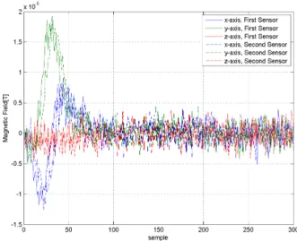
The Figures 2, 3 and 4 show the data generated to simulate sensors reading for cases 1, 3 and 5.

0 50 100 150 200 250 300 −1 −0.5 0 0.5 1 1.5x 10 −8 Magnetic Field[T] sample

x−axis, First Sensor y−axis, First Sensor z−axis, First Sensor x−axis, Second Sensor y−axis, Second Sensor z−axis, Second Sensor

Fig. 2. Readings from the sensors for case 1

We can see that the sketches illustrating the readings of the magnetic sensors are changing. The difference between Fig.2 and Fig.3 depends on the velocity where the increase in velocity decreases the number of samples, while the difference between Fig.3 and Fig.4 depends on the distance between the vehicle and the sensors, where the large distance results in a weaker signal and a reduced SNR.

3.2 State Estimation

The estimation steps mainly depend on finding the solu-tion to the following optimizasolu-tion problem

ˆ x=argminxVN W LS(x) VN W LS(x) = N X k=1 2 X sensor=1 (y_sensor,k−hsensor,k(x))T R−1(y_sensor,k−hsensor,k(x))

where ˆxare the estimated stats which minimize the cost functionV(x),y_sensoris the sensor measurement,hsensor

is the sensor model in (6) (without B0) and R is the

covariance matrix.

The optimization problem was solved using the algorithm propose in Wahlstr¨om [2010], Alimi [2009] and Gustafsson [2010] based on nonlinear weighted least squares method (NWLS). The algorithm was initiated using the values given in columnini. The estimation results for the previous cases are presented in the Table 2.

Table 2. Simulation Results

Case ini. 1 2 3 4 5 rx _-10 _-4.994 _-5.006 _-4.99 _-4.998 _-4.99 ry 3 2.002 1.982 2.002 1.199 4.08 rz ₁ _0.003 _-0.006 _0.012 _0.001 _0.00 mx ₁ _0.499 _0.498 _0.494 _0.500 _0.51 my ₁ _0.500 _0.501 _0.494 _0.500 _0.48 mz ₁ _0.102 _0.098 _0.100 _0.100 _0.14 vx 12 4.995 15.004 19.968 19.992 20.06 vy ₁ _-0.001 _0.047 _-0.033 _0.004 _-0.28 vz ₁ _0.000 _0.015 _-0.030 _-0.007 _0.11 3.3 Discussion

The estimation results for all cases reveal a very good convergence to the states values used in the data creation. The estimation takes different iteration cycles depending on the case to be estimated. Moreover, in case 5, where the vehicle was far from the sensors and the SNR is low, the estimation algorithm still converges nicely to the states.

(4)

In some cases which are not considered in our simulation cases the estimation algorithmdivergeswhen the vehicle passes very close to the sensors. In these cases we violate a main condition for the magnetic sensor model, which is the distance between the vehicle and the sensors should be greater than the width of the magnetic dipole representing the vehicle itself. In other words, we could not estimate a long vehicle passing close to the sensor using that magnetic sensor model. In that case, we should sub-divide these kind of vehicles into multi-magnetic dipoles, see Wahlstr¨om [2010]. In addition, installing the sensors right in the middle of the road would violate a requirement of the magnetic dipole model validity.

There are many articles in which two magnetic sensors are used to detect the vehicle and to determine the velocity easily by using the cross-correlation between records for both sensors and the distance between them, see Karpis [2012]. The maximum cross-correlation of the sensors readings for case 1 occurs at lags 20, i.e 20Ts s. That

means, the vehicle which passed the first sensor would pass the second one by that time. Where Ts = 0.01 and

1m separates the sensors, vehicle velocity is 5 m/s. The maximum cross-correlation for case 3 occurs at lags 5, which means that the vehicle velocity is 20m/s. Lastly, the maximum cross-correlation for case 5 occurs at lags 5. That means the vehicle velocity is 20m/s.

Although it is easer to estimate the velocity using cross-correlation (regardless the errors may occur due to the error in sampling rate and/or the distance between the sensors), we prefer to use NWLS method, as not only the velocity would be determined but also vehicle magnetic moment and position in the x, y and z axes. Vehicle position is a very important factor if we would aim to warn vehicles coming on the other side of a road to avoid a head-on collisihead-on, or would aim to track vehicle within a sensor network. Besides, we can use both estimation methods in states estimation. A cross-correlation is used as first phase to estimate a good initial velocity guess which can further used inNWLS method as a second phase.

Finally, The sensors setup is very important to assume perfect results. In Wahlstr¨om [2010], a calibration of the reference frame is performed using accelerometer and the magnetic sensor as a compass. Fig.5 and Fig.6 simulate the readings from the two sensors when yaw (Ψ) and pitch (θ) angles of the second sensors are changed from 0 to 30◦ by a step size of 5◦. This change affects x and y axes readings in the first case and x and z readings in the second one. Case 1 is simulated again with both yaw and pitch angles equal to 15◦. The achieved results, using the same initial values with angles initial values of 0o, are given in Table 3 while the results without considering the angles deviation within the estimation algorithm are depicted in Table 4.

Table 3. Simulation Result

Case rx _ry _rz _mx _my

1 -4.98 1.98 0.00 0.49 0.49

mz _vx _vy _vz _θ _Ψ

0.09 4.98 0.00 0.00 14.83 14.72

Fig. 5. Changing yaw angle of the second sensor

Fig. 6. Changing pitch angle of the second sensor Table 4. Simulation Result without considering

the angles

Case rx _ry _rz _mx _my

1 -4.06 1.49 0.157 0.30 0.28

mz _vx _vy _vz _θ _Ψ

0.002 4.079 0.15 -0.18 -

-The previous tables reveal that the results in the case where the angles deviation effect is ignored are not as accurate as the case where it is considered. In the real experiment, emphasis has been on the accurate alignment of the sensor, thus perfect alignment is assumed as shown in Fig.7.

4. REAL LIFE EXPERIMENTS

4.1 Setup and Data Acquisition

The wireless sensor nodes for the traffic monitoring system are depicted in Fig. 8. These RMUs are only 7 millimeter high and can be glue attached to the surface. Since they are embedded into the road markings as an additional

(5)

Fig. 7. Collecting data using RMUs prototype

protection, the units sustain snow ploughs and are easily and fast installed on the road surface.

Fig. 8. Integrated RMU, 140mm wide and long and 7mm high

A pre-production prototype which is not fully inte-grated contains a Honeywell 2-axis magnetic sensor type HMC6042 to measure x and y axis and 1-axis magnetic sensor type HMC1051 to measure z axis, were used to collect data from real traffic on a rural road close to LTU, as shown in Fig.7. The 2-axis sensor itself has 225 times amplification, see Honeywell [2007], and then an external amplification was used to amplify 25.5 times more, while the 1-axis sensors amplified 102×25.5 times by an external amplification.

Due to a high sampling rate of 16384Hz a huge amount of data was collected in four measurement sessions in more than one hour for each.

4.2 Estimation Of Vehicle States Based on Real Data

After we applied a modified detection algorithm, see Cheung [2007], to the measurements many signatures for passing vehicles were extracted. The important point is that the two sensors were synchronized with each other, so we applied the detection algorithm on the readings of both sensors at the same time. One of the detection signals for both sensors is shown in Fig.9 which refers to a Volvo SUV passing by.

Table 5 shows the results obtained by applying the dis-cussed estimation algorithm to estimate the states of the

Fig. 9. The Volvo SUV magnetic signature

Volvo SUV. The initial values have been chosen based on our knowledge of sensor sensitivity, road width and speed.

Table 5. Result of states Estimation

case ini. Volvo (SUV) BMW Toyota Scania 114L

rx -7 -15.712 -13.177 16.52 -21.8 ry ₃ _2.04 _0.626 _3.54 _8.20 rz ₁ _1.062 _1.697 _-6.68 _-6.32 mx _0.05 _-0.072 _-0.0722 _-0.095 _-1.69 my _-0.05 _-0.007 _-0.008 _-0.006 _-0.176 mz 0.05 0.0076 0.0106 0.037 -0.497 vx ₁₅ _22.9 _18.23 _-24.05 _18.37 vy ₀ _1.460 _2.852 _7.59 _1.047 vz ₀ _-1.111 _-1.428 _7.64 _5.30 0 50 100 150 200 250 300 350 400 −4 −2 0 2 4x 10 −10 x−axis real signature estimated signature 0 50 100 150 200 250 300 350 400 −4 −2 0 2 4x 10 −10 y−axis 0 50 100 150 200 250 300 350 400 −0.5 0 0.5 1x 10 −10 z−axis sample

Fig. 10. Estimation comparison of the Volvo case

Fig.10 shows a comparison between the real sensor signals and the reconstructed signals given by substituting the estimation results in (4)(withoutB0). The Figure shows a

good fitting between the real and the reconstructed signals. Table 5 contains three additional estimation cases. The estimation results revealed that the Volvo and the BMW were coming from left to right due to thenegative value of rx _{and the} _positive _{value of} _vx_{. They show also that the}

(6)

Table 6. Standard deviation of Estimated States

case Volvo BMW Toyota Scania 114L

rx _0.214 _0.116 _0.568 _0.574 ry _0.133 _0.073 _0.206 _0.267 rz _0.155 _0.089 _0.268 _0.213 mx _0.030 _0.002 _0.01 _0.13 my _0.0009 _0.0006 _0.0017 _0.022 mz _0.0006 _0.0005 _0.0041 _0.039 vx _0.301 _0.155 _0.877 _0.471 vy _0.186 _0.103 _0.382 _0.140 vz 0.220 0.122 0.362 0.177

while the Toyota was coming in the opposite direction due to the positive value of rx _{and the} _negative _{value of} _vx_.

Moreover, we are almost sure that the Toyota was passing on the other lane because the value of ry _{is bigger than}

those of the previous ones. Besides, we can not be very confident about the estimation results for the Scania114L. That was expected as the vehicle was too long compared to distance to the sensors position as we explained earlier. After all, its direction is still able to be recognized (due to rx _and_vx_sign).

The standard deviation of the estimated states of the four cases are depicted in the Table 6. Assume that the noise of magnetometer is white Gaussian, i.e. its samples are i.i.d and are normally distributed with zero mean. As a result

Rwas used equal to 10−22_I_T2_{which was measured during}

the target absence after removing the bias caused by earth magnetic field.

5. CONCLUSIONS

In order to get safe roads, vehicle tracking can provide substantial information. In this paper, a vehicle tracking scheme was successfully evaluated by determine vehicle position, velocity and magnetic moment. This scheme is achieved by using readings from two 3-axes magnetic sensors. The tracking was performed in both simulation and real life experiments. The real life experiments show a good performance for vehicles on the same side of the road as the installation spot of the sensors, while they give less performance for vehicles on the other lane. Large vehicles create difficulties for the tracking scheme due to an invalidation of single dipole moment model for such vehicles. The velocity and position results gave valuable information about vehicle trajectory while the magnetic moment can be used to reveal vehicle types. The results motivate further and longer tests with a secondary measurement device as ground truth. Test with fully integrated production hardware are now planned and will be conducted in the near future.

6. ACKNOWLEDGMENT

Many thanks to my colleagues Khalid Atta and Roland Hostettler for their help and support. Also the effort of Geveko ITS A/S for conducting the experiments and pro-viding the experimental data are gratefully acknowledged.

REFERENCES

A. Eidehall, J. Pohl, F. Gustafsson and J. Ekmark. ”To-ward autonomous collision avoidance by steering”

Intel-ligent Transportation Systems, IEEE Transactions on,

volume. 8, number. 1, pages 84–94, 2007.

W. Birk, E. Osipov and J. Eliasson. ”iRoad–cooperative road infrastructure systems for driver support”. in Proceedings of the 16th ITS World Congress, 2009. T. Phan, B. Kwan, and L. Tung. ”Magnetoresistors for

vehicle detection and identification”. in Systems, Man, and Cybernetics, 1997. Computational Cybernetics and Simulation., 1997 IEEE International Conference on, volume. 4. IEEE, 1997, pages 3839–3843.

S. Cheung and P. Varaiya, ”Traffic surveillance by wireless sensor networks:Final report”. California PATH Pro-gram, Institute of Transportation Studies, University of California at Berkeley, 2007.

O. Karpis, ”Sensor for vechiles classification” pages 785– 789, 2012.

M. Birsan, ”Non-linear kalman filter for tracking a mag-netic dipole” inProceedings of the International

Confer-ence on Marine Electromagnetic(MARELEC04), 2004.

M. Birsan, ”Unscented partical filter for tracking a magnetic dipole target” in OCEANS, 2005. Proceedings of MTS/IEEE. IEEE, pages 1656–1659, 2005.

N. Wahlstr¨om, J. Callmer, and F.Gustafsson, ”Magne-tometer for tracking metallic target”, in Information

Fusion(FUSION), 2010 13th conference on, IEEE, 2010

pages 1–8.

N. Wahlstr¨om, ”Target tracking using maxwells equa-tions”, p. 87, 2010.

M. Caruso and L. Withanawasam, ”Vechile detection and compass application using AMR magnetic sensors”,in

Sensors Expo Proceedings, Volume 477, 1999.

R. Alimi, N. Geron, E. Weiss and T. Ram-Cohen, ”Ferro-magnetic mass localization in check point configuration using Levenberg marquardt algorithm”, Sensors, Vol-ume 9, number 11, pages 8852–8862, 2009.

D. T¨ornqvist, statistical fault detection with applications to IMU disturbances”, Ph.D dissertation, Link¨oping, 2006.

F. Gustafsson, ”Statiscal sensor fusion”, Studentlittera-ture, 1 edition, 2010.

Honeywell co. ”2-axis magnetic sensor circuit HMC6042”, 2007.