Abstract—Accurate prediction of streamflow plays a pivotal role for effective reservoir system operations. Specifically, streamflow forecasting provides valuable information for reservoir operators to make critical decisions on water release amount to maximize reservoir storage benefits considering tradeoffs among flood control, municipal water supply, irrigation, hydropower etc. This task, however, has posed daunting challenges due to the complex mechanisms of the physical-based processes as well as the influence of uncontrollable factors. Hence, developing a robust mathematically driven model - in tandem with the supervision of proficient hydrologists for validation purposes - to ensure an accurate forecasting of discharge flows could be of paramount importance. To this end, a deep learning framework using a variation of recurrent neural networks called Long Short-term Memory (LSTM) network, for an accurate prediction of streamflow is presented and evaluated - without losing any generality - for a watershed outlet at the United States Geological Survey (USGS) gauge station neighboring Hempstead within the poorly-gauged region of Brazos basin in Texas with temporal coverage of 2007-2010. In this work, the antecedent precipitation observations and the climate variability indices have been utilized as the potential predictors. Our model is, however, scalable and transferable to be deployed across variant basins with various drainage areas. We, herein, assessed the performance of our predictive model via the Pearson correlation ( ) and the Nash–Sutcliffe model efficiency (NSE) coefficients between the predicted and observed streamflow, achieving and NSE of 0.9542 and 0.8859, respectively.
Index Terms—Streamflow, deep learning, long short-term memory, basin delineation.
I. INTRODUCTION
Decision making relative to water resources requires the characterization and perception of the heterogeneous - and often chaotic - environmental systems, and accordingly, a well-grounded scheme for water budget management. However, a reliable planning and management of water resources to ensure sustainable use of watershed budgets would necessitate precise and robust models to enable the scientist to examine the potential players subscribing towards
Manuscript received May 2, 2019; revised July 23, 2019.
Hamidreza Ghasemi Damavandi, Dimitrios Stampoulis, Reepal Shah, Yuhang Wei, and John Sabo are with Future H2O, the Office of Knowledge Enterprise Develepment, Arizona State University, Tempe, AZ, USA (e-mail: {hghasemi, dstampou, Reepal.Shah, John.L.Sabo, yuhang.wei}@asu.edu).
Dragan Boscovic is with the Center of Assured and Scalable Data Engineering (CASCADE), Arizon.
the streamflow patterns. Conventional physically-based models have long been applied to simulate the hydrological regimes. Nevertheless, characterized by the complexity, non-linearity and the uncertainty in variable estimation, these models have often failed to meet the practical needs for a dynamic hydrological analysis. These issues are often plagued while the data are erroneous or the environmental noise leaks into the observations which would, consequently, deteriorate the model performance. Moreover, as [1] declares, physical-based models require a large amount of data for calibration and validation purposes, and thus, are computationally intense. We, however, aim at developing a nimble data-driven model, which could discover the underpinnings of the input and output variables efficiently using sufficient amount of data. Additionally, this model needs to be robust enough to hold its promise even in the presence of noise.
Data-driven models, and deep learning architectures in particular, have recently gained immerse applicability in hydrologic modeling as the underlying inter-relationships among the parameters are learnt, merely, through the data in an automated manner without any external effort exerted by human experts [2]-[4]. These models often out-perform the statistical models, as no prior model assumption for the input-output relation is required (examples of statistical methods can be found at [5]-[11]). An appropriately designed deep learning architecture would in turn enable us to extract the governing physical-based inter-relationships where the learning parameters are adjustable [12]. Moreover, these models are in principle scalable, leading to fast-computing engines to process variant amount of data efficiently. Backed by advanced optimization theories, and the transferable dynamics to be deployed in variant hydrological conditions and across different basins, these models have now emerged as powerful alternatives to the conventional hydrological models. Specifically, for the purpose of this work, we compare our proposed data-driven model against the Catchment-based physically explicit Macro-scale Floodplain (CaMa-Flood) model [13]-[16], a hydrological model designed to simulate the hydrodynamics in continental-scale rivers. Interested readers are referred to [17].
Several studies have investigated the capability of artificial intelligence to forecast streamflow. To name a few, Liu et. al. 2017, [18] examined the ability of the Relevance Vector Machine (RVM) model and its applicability for long-term streamflow forecasting where the Dahuofang (DHF) Reservoir in Northern China and the Danjiangkou (DJK)
Accurate Prediction of Streamflow Using Long
Short-Term Memory Network: A Case Study in the Brazos
River Basin in Texas
Reservoir in Central China were chosen as the study sites for the model evaluation. The results in this work, exhibited the RVM as an effective model for long-term stream flow forecasting. Asefa et al. 2006, [19] presented Support Vector Machines (SVMs) to forecast flows at two time scales: seasonal flow volumes and hourly stream flows. On a similar study, Lin et al. 2006, [20] compared the performance of autoregressive moving-average (ARMA) models with SVM. Their results demonstrate the prominent potential of SVM for long-term stream flow prediction.
The objective of this study is, therefore, to propose a fully automated framework to forecast the stream flow of a desired outlet of a watershed both for short- and long-term purposes based on past meteorological input. We work this out via performing basin delineation and extracting the potential predicting cells within the gridded digital elevation model (DEM) of the basin. We exploit the antecedent precipitation observations – as the fundamental input variable for the hydrological modelling of river basins [21] - and the indices denoting the climate variability as the potential predictors for stream flow forecasting.
The rest of the paper is organized as follows: Section II briefly introduces the region of study for this work. The dataset used in this study is explained in Section III. Section IV expatiates the proposed method to detect the potential contributive cells toward the streamflow forecasting at the location of an outlet. The results are shown in Section V. Section VI concludes the paper.
II. REGION OF INTEREST:WATERSHED OUTLET LOCATED
NEAR HEMPSTEAD IN BRAZOS BAISIN,TEXAS
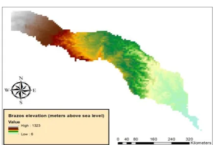
Fig. 1. The digital elevation model (DEM) of the Brazos basin in Texas. We investigate the outlet located at 30.09375o (latitude) and -96.21875o (longitude) in which most of the cells drain into it. Note that, this topography is originally a 1 km SRTM DEM and this map is the 0.0625 degree spatially. averaged version.
Brazos basin is the 11-th longest river in the United States and the second biggest basin by area within Texas with the size of 45,000km2 flowing 840 mile from the confluence of Salt and Double Mountain forks in Stonewall County to the Gulf of Mexico having the largest average annual flow volume among the rivers in Texas (Fig. 1). Note that, this topography is originally a 1 km Shuttle Radar Topography Mission (SRTM) DEM and this map is the 0.0625 degree spatially averaged version. The afore-mentioned characteristics turn this basin into an appealing case study for scientific scrutiny. We explore the watershed outlet with the
coordinates of 30.09375o (latitude) and -96.21875o (longitude), located at the lower reach of the basin. Most of the cells within the basin would drain into this outlet, providing us with sufficiently enough data points to train our learning architecture.
III. DATASET
The precipitation data utilized in this work is extracted from the publicly available Livneh’s database [22]. This database contains the Conterminous United States (CONUS) near-surface gridded meteorological and derived hydrological data with daily temporal resolution spanning from 1915-2011, at the spatial resolution of 0.0625o and with a spatial coverage of 21.21875-52.90625 (latitude), 235.4688E-293.0312E (longitude). For the purpose of this study, we focus our investigations on the time interval of 2007 to 2010.
Motivated and guided by the prolific literature on the effect of climate variability over the streamflow patterns [23]-[28], we included the Pacific Decal Oscillation index (PDO), – download at [29] - El Niño–Southern Oscillation (ENSO) activity measured via Nino 3.4, - downloaded at [30] - Pacific/North American Index (PNA), Arctic Oscillation (AO), North Atlantic Oscillation (NAO), Antarctic Oscillation (AAO), – downloaded at [31] - as the potential climatological predictors. Finally, streamflow was captured from the USGS gauge station #08111500 (Brazos River near Hempstead, Texas) [32].
IV. METHODOLOGY
utilized for miscellaneous time series prediction as the interdependence could be of either short or long term within the data points across different time stamps. LSTMs, however, holds promise to capture any temporal inter-dependency. Due to the ability of keeping the information from the past input data points, LSTM networks are often considered as ideal candidates for both short and long time series prediction problems (short and long term streamflow prediction in this work). Ultimately, these predictors will be used to train the proposed LSTM network. We extract the contributive cells via applying a threshold on the flow accumulation pattern of the basin. Let us assume,
n
cells are selected as the contributive cells, and according to Table I, each cell contains seven time-series as the feature. Therefore, there exists:
N
n
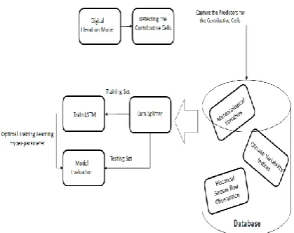
(Precipitation pattern for each cell) + 6 (climate variability indices) + 1 (one-lag streamflow) (2)Fig .2. Block-diagram illustrating the outline to develop the learning architecture for streamflow prediction. Once the potential predicting cells are extracted from the DEM of the watershed, the corresponding predictors are then retrieved from the database for training.
Number of time-series as the potential predictors. As noted earlier, each of these time-series is of length of four years (2007-2010), or 1461 days. Equivalently, at each timestamp like
t
, we haveN
number of features to forecast the streamflow att
. Now, if we choose to train the network usingM
number of days, we have a training set of sizeM
N
. The training data is now “sequentially” fed into the network, i.e. at each time stamp one row containingN
features are used to train the network for the streamflow value at the corresponding timestamp. In this workn
, or the number of selected cells, is 133, and thus,N
140
. The proposed deep learning network is shown in Fig. 3. This network consists of an input layer with 140 neurons, stacked block of LSTM cells with ten hidden layers followed by a fully connected layer. Each LSTM cell consists of 300 memory units. The back-prorogation optimization to train the weights across the network is performed using Adam optimizer [37]. Dropout module [38] is employed between each layer to avoid the over-fitting issue [39] and further improvement in prediction accuracy. Ultimately, the performance of the network is evaluated over the testing data and using the Pearson correlation and Nash–Sutcliffe modelefficiency coefficients. We trained the machine using the first 1000 days (~68% of total days) and tested against the remaining 461 days (~32% of total days). The programming language used for this work is the free and open source Python 3.7 [40]. The deep learning frameworks were implemented using the well-known Tensorflow [41] and Keras [42] libraries. Calculations were mainly performed via Sckit-learn [43] and Numpy [44] packages. All analysis is carried out on an Ubuntu-based machine with Intel Xeon CPU 6136 processor.
Fig. 3. The proposed deep learning framework. This network consist of ten stacked LSTM blocks followed by a fully connected layer. To evade the
over-fitting issue, we deployed dropout module between each layer.
TABLEI:POTENTIAL PREDICTORS FOR STREAMFLOW PREDICTION
Feature Name Abbreviation
Precipitation PRC
Pacific Decadal Oscillation Index
PDO
Pacific/North American Index
PNA
Arctic Oscillation AO
North Atlantic Oscillation NAO
El Niño–Southern Oscillation
ENSO
Antarctic Oscillation AAO
Stream flow at the previous time stamp
SF_Lag
A. How to Detect the Contributive Cells?
In this section, we expatiate the strategy to determine the contributive cells for streamflow prediction at the outlet location. It is worth mentioning that, the key distinction of our proposed method is that we use a sub-set of the cells within the watershed towards an accumulation of flow at the location of the outlet. We, herein, propose a systematic method to detect these cells and build the deep learning architecture over them. Thus, the following six-step strategy is suggested:
1) As indicated earlier, the process begins by capturing the DEM of the basin using ArcGIS.
2) DEMs often suffer from depressions, or pits, which are areas of a landscape wherein flow ultimately terminates without reaching an ocean or the edge of a DEM. We fill these depressions using the fill tool in Hydrology toolbox.
(latitude) and -96.21875o (longitude).
4) Basin delineation is the task of creating boundary defining the contributing area, or the geographical cells, for a particular outlet within a watershed via analyzing flow directions within the DEM of a basin. Delineation is part of the process known as watershed segmentation, i.e., dividing the watershed into discrete land and channel segments to analyze watershed behavior. Basin delineation is often considered as the key point to study of the potential development of water resources in a basin. Interested readers are referred to [45], [46] for a comprehensive note on basin delineation using DEM. We first delineate the basin around the outlet point to detect the boundary for the potential contributive cells towards an accurate approximation of stream flow. Basin delineation is usually performed using ArcGIS. Instead, we accomplished this task via the use of a python-based toolbox. Fig. 4 shows the delineated watershed for the investigated outlet.
Fig. 4. Delineated watershed surrounding the outlet located at 30.09375o (latitude) and -96.21875o (longitude).
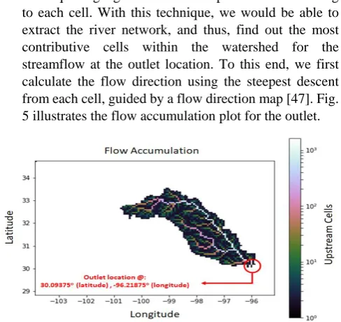
5) For the next step, we perform the flow accumulation technique to gauge the number of upstream cells draining to each cell. With this technique, we would be able to extract the river network, and thus, find out the most contributive cells within the watershed for the streamflow at the outlet location. To this end, we first calculate the flow direction using the steepest descent from each cell, guided by a flow direction map [47]. Fig. 5 illustrates the flow accumulation plot for the outlet.
Fig. 5. Flow accumulation plot of the outlet located at 30.09375o (latitude) and -96.21875o (longitude).
6) To extract the river network, we apply a threshold on the flow accumulation pattern to exclude off the cells with low number draining cells. The remaining cells are then
treated as the contributive cells for the streamflow of the outlet.
Fig. 6. Contributive cells resulted from thresholding the flow accumulation distribution of the watershed for the outlet located at 30.09375o (latitude) and
-96.21875o (longitude).
Once the potential cells are detected, we train a many-to-one deep learning architecture to map the hydrological parameters of these cells to the streamflow of the outlet. This six-step strategy is summarized in Fig. 7.
Fig. 7. The six stages of extracting the potential predicting cells within a basin for the streamflow prediction at the location of a pre-set outlet of a watershed. We solely need the gridded digital elevation model of the basin to kick off the procedure.
V. RESULT
evaluation metrics.
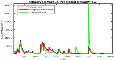
Fig. 8. Observed versus the predicted streamflow time-series for the outlet located at 30.09375o (latitude) and -96.21875o (longitude) within the downstream watershed of Brazos basin in Texas. The streamflow has been
calculated as 3
m
s
.A. Evaluation Metrics
For further clarification of our analysis, we herein, define the evaluation metrics used in this work. The Nash–Sutcliffe model efficiency coefficient between the observed and model-derived flow is defined as following:
2 0 1
2
0 0
1
(
)
1
(
)
T
t t
m t
T t
t
s
s
NSE
s
s
(1)where
s
0
is the mean of observed discharges, and
s
m is modeled discharge.s
0t is observed discharge at time t. This coefficient ranges from
to 1, corresponding to the worst and best prediction performance. NSE of 0.8859 certifies the high quality of our predictive model.The Pearson correlation coefficient between
s
m ands
0 isdefined as:
0 0 0
cov(
,
)
(
,
)
m m m
s s
s s
s s
(2)where the
cov(.)
and
(.)
are the covariance and standard deviation operators, respectively.TABLE II: COMPARISON BETWEEN THE PROPOSED DEEP LEARNING NETWORK AND CAMA-FLOOD FOR STREAMFLOW PREDICTION USING PEARSON CORRELATION AND NASH–SUTCLIFFE MODEL EFFICIENCY COEFFICIENTS
Metric Proposed Network CaMa-Flood
0.9542 0.4814NSE
0.8859 -1.1299VI. CONCLUSION
Conventional models exploring the physical mechanics of environmental events have long disclosed invaluable information to scientists towards a precise explanation for these events. These models, however, are limited in broader applications due to their complex nature and tedious
validation processes. To this end, data-driven techniques have been deployed to replicate the multi-scale conventional environmental as well as hydrological models [18], [19], [20], [48]-[51]. These techniques benefit from advanced optimization theories to delve into the data and unravel the intrinsic relationships of the parameters but in an efficient manner. Furthermore, with the advent of deep learning – as a more sophisticated version of machine learning techniques – scientists are now able to probe the data in an automated manner, without an explicit need for manual feature engineering, as was the case with the conventional machine learning techniques.
In this work, for the very first time - to the best of our knowledge - we propose an automated learning pipeline to forecast the stream flow within a basin using the digital elevation topography and the state-of-the-art deep learning framework, i.e. Long short-term memory network. Without using any generality, we applied our network over the flow observations collected at an outlet located at the bottom of the Brazos basin in Texas and validated via the USGS gauge station near Hemsptead. This method, however, is generic and could be easily harnessed for any basin. This is actually the key distinction of deep learning models i.e. both scalability and tunability for miscellaneous scenarios. The metrics for the evaluation are the Pearson correlation (
) and Nash–Sutcliffe model efficiency (NSE
) coefficients between the observed and predicted flows achieving(.)
0.9542
(P-value < 0.00005) andNSE
0.8859
. Additionally, our proposed model outperformed CaMa-Flood, the model commonly used in hydrologic community for streamflow simulation. The results presented in this work, denote the prominent capacity of deep learning for an accurate prediction of discharges, and of course, an efficient alternative to the conventional hydrological models. Besides this capacity, data-driven models exhibit great potential to capture anthropogenic impacts such as water use and reservoir operation, which is difficult - if not impossible - to be reflected in distributed hydrological models.CONFLICT OF INTEREST
The authors declare no conflict of interest. AUTHOR CONTRIBUTIONS
HGD contributed significantly towards the data preparation as well as the algorithm development and its implementation; HGD, RS, DS and YW contributed significantly towards drafting the manuscript, verifying the findings of the work and the related interpretation of the results; DB and JS supervised the project and have been significantly involved in revising the results for the intellectual content as well as providing critical feedback; all authors had approved the final version.
ACKNOWLEDGMENT
REFERENCES
[1] Y.-F. Sang, “Improved wavelet modeling framework for hydrologic time series forecasting,” Water Resources Management, vol. 27, no. 8, 2013, pp. 2807-2821.
[2] M. Jean and J.-R. Dreuzy, “Prospective interest of deep learning for hydrological inference,” Groundwater, vol. 55, no. 5, 2017, pp. 688-692.
[3] A. Haytham et al., “Urban water flow and water level prediction based on deep learning,” Joint European Conference on Machine Learning and Knowledge Discovery in Databases, Springer, Cham, 2017. [4] P. Liu et al., “SVM or deep learning? A comparative study on remote
sensing image classification,” Soft Computing, vol. 21, no. 23, 2017, pp. 7053-7065.
[5] A. Geetha and G. M. Nasira, “Time-series modelling and forecasting: Modelling of rainfall prediction using ARIMA model,” International Journal of Society Systems Science, vol. 8, no. 4, 2016, pp. 361-372. [6] G. Anosh and E. P. Mishra, “Time series analysis model to forecast
rainfall for Allahabad region,” Journal of Pharmacognosy and Phytochemistry, vol. 6, no. 5, 2017, pp. 1418-1421.
[7] R. D. Stern and R. Coe, “A model fitting analysis of daily rainfall data,” Journal of the Royal Statistical Society: Series A (General), vol. 147, no. 1, 1984, pp. 1-18.
[8] C. E. Richard and H. S. Wheater, “Analysis of rainfall variability using generalized linear models: A case study from the west of Ireland,” Water Resources Research, vol. 38, no. 10, 2002, pp. 10-11. [9] A. K. Mangaraj, L. N. Sahoo, and M. K. Sukla, “A Markov chain
analysis of daily rainfall occurrence at western Orissa of India,” Journal of Reliability and Statistical Studies, vol. 6, no. 1, 2013, pp. 77-86.
[10] I. Lily et al., “Applications of statistical methods for rainfall prediction over the Eastern Thailand,” in Proc. the International Multi Conference of Engineers and Computer Scientists, vol. 3, 2010. [11] J.-Y. Ho and K. Lee, “Grey forecast rainfall with flow updating
algorithm for real-time flood forecasting,” Water, vol. 7, no. 5, 2015, pp. 1840-1865.
[12] G. Ian, Y. Bengio, and A. Courville, Deep Learning, MIT Press, 2016. [13] Y. Dai et al., A physically based description of floodplain inundation dynamics in a global river routing model,” Water Resources Research, vol. 47, no. 4, 2011.
[14] Y. Dai et al., “Analysis of the water level dynamics simulated by a global river model: A case study in the Amazon River,” Water Resources Research, vol. 48, no. 9, 2012.
[15] Y. Dai, G. A. M. Almeida, and P. D. Bates, “Improving computational efficiency in global river models by implementing the local inertial flow equation and a vector‐based river network map,” Water Resources Research, vol. 49, no. 11, 2013, pp. 7221-7235.
[16] Y. Dai et al., “Regional flood dynamics in a bifurcating mega delta simulated in a global river model,” Geophysical Research Letters, vol. 41, no. 9, 2014, pp. 3127-3135.
[17] Cama. [Online]. Available:
http://hydro.iis.u-tokyo.ac.jp/~yamadai/cama-flood/index.html [18] Y. Liu et al., “Long-term streamflow forecasting based on relevance
vector machine model,” Water, vol. 9, no. 1, 2017, p. 9.
[19] A. Tirusew et al., “Multi-time scale stream flow predictions: The support vector machines approach,” Journal of hydrology, vol. 318, no. 1-4, 2006, pp. 7-16.
[20] J.-Y. Lin, C.-T. Cheng, and K.-W. Chau, “Using support vector machines for long-term discharge prediction,” Hydrological Sciences Journal, vol. 51, no. 4, 2006, pp. 599-612.
[21] T. A. J. G. Sirisena et al., “Effects of different precipitation inputs on streamflow simulation in the Irrawaddy River Basin, Myanmar,” Journal of Hydrology: Regional Studies, vol. 19, 2018, pp. 265-278. [22] L. Ben et al., “A long-term hydrologically based dataset of land surface
fluxes and states for the conterminous United States: Update and extensions,” Journal of Climate, vol. 26, no. 23, 2013, pp. 9384-9392. [23] R. Kabir, W. W. Hsieh, and A. J. Cannon, “Daily streamflow forecasting by machine learning methods with weather and climate inputs,” Journal of Hydrology, vol. 414, 2012, pp. 284-293.
[24] B. H. Donald, “Climatic influences on streamflow timing in the headwaters of the Mackenzie River Basin,” Journal of Hydrology, vol. 352, no. 1-2, 2008, pp. 225-238.
[25] G. K. C. Clarke, “Glacier‐mediated streamflow teleconnections to the Arctic Oscillation,” International Journal of Climatology: A Journal of the Royal Meteorological Society vol. 26, no. 5, 2006, pp. 619-636. [26] W. Y. Jon, P. H. Whitfield, and A. J. Cannon, “Influence of pacific
climate patterns on low-flows in British Columbia and Yukon, Canada,” Canadian Water Resources Journal, vol. 31, no. 1, 2006, pp. 25-40.
[33] W. H. Zhang and D. R. Montgomery, “Digital elevation model grid size, landscape representation, and hydrologic simulations,” Water Resources Research, vol. 30, no. 4, 1994, pp. 1019-1028.
[34] S. Martin, R. Schlüter, and H. Ney, “LSTM neural networks for language modeling,” presented at ThirteenthAnnual Conference of the International Speech Communication Association, 2012.
[35] G. A. Felix, J. Schmidhuber, and F. Cummins, “Learning to forget: Continual prediction with LSTM,” 1999, pp. 850-855.
[36] M. Tomáš et al., “Recurrent neural network based language model,” presented at Eleventh Annual Conference of the International Speech Communication Association, 2010.
[37] K. P. Diederik and J. Ba, “Adam: A method for stochastic optimization,” 2014.
[38] B. Jimmy and B. Frey, “Adaptive dropout for training deep neural networks,” Advances in Neural Information Processing Systems, 2013. [39] D. Tom, “Overfitting and undercomputing in machine learning,” ACM
Computing Surveys, vol. 27, no. 3, 1995, pp. 326-327.
[40] M. F. Sanner, “Python: A programming language for software integration and development,” J Mol Graph Model, vol. 17, no. 1, 1999, pp. 57-61.
[41] A. Martín et al., “Tensorflow: A system for large-scale machine learning,” 12th {USENIX} Symposium on Operating Systems Design and Implementation ({OSDI} 16), 2016.
[42] G. Antonio and S. Pal, Deep Learning with Keras, Packt Publishing Ltd, 2017.
[43] P. Fabian et al., “Scikit-learn: Machine learning in Python,” Journal of Machine Learning Research, vol.12, 2011, pp. 2825-2830.
[44] D. Walt et al., “The NumPy array: A structure for efficient numerical computation,” Computing in Science & Engineering, vol. 13, no. 2, 2011, p. 22.
[45] O. L. Palacios-Velez and B. Cuevas-Renaud, “Automated river-course, ridge and basin delineation from digital elevation data,” Journal of Hydrology, vol. 86, no. 3-4, 1986, pp. 299-314.
[46] P. J. Soille and M. M. Ansoult, “Automated basin delineation from digital elevation models using mathematical morphology,” Signal Processing, vol. 20, no. 2, 1990, pp. 171-182.
[47] S. Holger, O. Marinoni, and M. Hinderer, “A GIS-based method to calculate flow accumulation by considering dams and their specific operation time,” Computers & Geosciences, vol. 34, no. 6, 2008, pp. 635-646.
[48] D. H. Ghasemi and R. Shah, “A learning framework for an accurate prediction of rainfall rates,” 2019.
[49] D. H. Ghasemi et al., “Interpreting comprehensive two-dimensional gas chromatography using peak topography maps with application to petroleum forensics,” Chemistry Central Journal, vol. 10, no. 1, 2016, p. 75.
[50] D. H. Ghasemi et al., “Signal variability and data compression considerations for petroleum forensics in two-dimensional gas chromatography,” OCEANS 2017-Aberdeen, IEEE, 2017.
[51] D. H. Ghasemi et al., “Oil-spill forensics using two-dimensional gas chromatography: Differentiating highly correlated petroleum sources using peak manifold clusters,” presented at 2015 49th Asilomar Conference on Signals, Systems and Computers, 2015.
Copyright © 2019 by the authors. This is an open access article distributed under the Creative Commons Attribution License which permits unrestricted use, distribution, and reproduction in any medium, provided the original work is properly cited (CC BY 4.0).
Hamidreza Ghasemi Damavandi received his doctoral degree at the Department of Electrical and Computer Engineering, the University of Iowa, summer 2016. Prior to Ph.D, he received his BS.c degree at the Department of Electrical and Computer Engineering, University of Tehran, summer 2013. His main research interest is to apply machine and deep learning strategies to mimic the environmental and
[27] D. J. Stephen and E. F. Wood, “Teleconnection between the Arctic Oscillation and Hudson Bay river discharge,”Geophysical Research Letters, vol. 31, no. 18, 2004.
[28] D. J. Stephen and E. F. Wood, “Decreasing river discharge in northern Canada,”Geophysical research letters, vol. 32, no. 10, 2005. [29] Jisao. [Online]. Available: http://research.jisao.washington.edu/pdo/ [30] Cpc. [Online]. Available:
https://www.cpc.ncep.noaa.gov/data/indices/sstoi.indices [31] Cwlinks. [Online]. Available: ftp://ftp.cpc.ncep.noaa.gov/cwlinks/ [32] Nwis. [Online]. Available:
hydrological events. He currently works as postdoctoral research associate at office of knowledge enterprise development, Future H2O, Arizona State University. He attempts to emulate the physical-based hydrological models via optimization theories as well as the deep machine learning tools. He held the same position at University of California- Los Angeles before joining ASU.
Reepal Shah is currently an assistant research scientist with Arizona State University. He received his PhD from IIT Gandhinagar in 2017. His current research are surrounding following areas: hydrology, climate variability and climate change impact assessment, and crop modeling.
Dimitrios Stampoulis received his doctoral degree from the Civil & Environmental Engineering Department of the University of Connecticut. He is currently a research scientist working at the Arizona State University. His primary research interests are directed toward investigating the potential for synergies between remote sensing science and hydrology as well as eco-hydrology in the aim of understanding the linkages and interactions between the water dynamics and different ecosystem processes. He uses hydrologic modeling, remote sensing observations and data integration techniques to assess the impact of climatic variability on freshwater availability globally.
Yuhang WeiYuhang Wei is currently a postdoctoral research associate with Arizona State University. He received his PhD and BEng from Hohai University in Water Conservancy and Hydropower Engineering. His research interests are water resources modeling and optimization, decision support tool.
Dragan Boscovic is the technical director of Center for Assured and Scalable Data Engineering (CASCADE) as well as the founder and director of Blockchain Research Lab at Arizona State University. His research interest is on the envisions, communicate and direct development of technologies, products and services in support of IoT smart spaces vision focusing on Smart City, Smart Office, eHealth and Mobility services and applications.