Page 84 www.ijiras.com | Email: [email protected]
On The Use Of Quantile Regression Technique For The Analysis
And Estimation Of The Determinants Of Wage Differential Of
Workers In Nigeria
O.A Fasoranbaku
Professor, Department of Statistics, Federal University of Technology, Akure, Nigeria
D.S Oluwadahunsi
Technologist,Department of Statistics, Federal University of Technology, Akure, Nigeria
G.O Daramola
Ph.D. Student, Department of Statistics, Federal University of Technology, Akure, Nigeria
I. INTRODUCTION
Linear regression can be described as representing the dependent variable as a linear function of one more independent variable(s), subject to random disturbance error. It estimates the mean value of the dependent variable for given levels of the independent variables. For the type of regression in which we may want to understand the central tendency in a dataset, the use of ordinary least square (OLS) is of paramount importance. OLS, however, losses its importance the moment an attempt is made to go beyond the median value or towards the extremes of a dataset. Quantile Regression was therefore introduced as a non-parametric method for modelling a variable of interest as a function of covariates. By estimating
the conditional quantiles rather than the mean, it gives a more complete description of the conditional distribution of the response variable than least square regression, and is especially useful in certain types of applications.
Quantile regression has appeared as an alternative to least squares in a wide range of applications. When the centre of the conditional distribution of a response variable Y, given a covariate vector X, is under investigation, median regression provides a consistent estimator of the conditional median without assuming a specific form for the conditional distribution. When other conditional quantiles, for example, the lower or upper tail of the conditional distribution, are of interest, quantile regression provides a way to directly estimate the interesting quantiles without assuming that such
Abstract: In this study, we attempted to analyze the determinants of wage disparity by applying quantile regression technique. The significant effect of factors influencing wage disparity such as gender, education, age and job tenure was carried out using Quantile Regression Technique. The stratified random procedure was used to select a sample data of one thousand one hundred and eleven (1111) workers from the Federal University of Technology Akure, Nigeria (FUTA). Strata and Gretl statistical packages were used for the implementation of the quantile regression procedure through the use of quantile (θ) values 0.05, 0.25, 0.5, 0.75 and 0.95. We found out that wage is positively related to age, gender and education at all quantiles. However wage is negatively related to job tenure at middle and higher quantiles but positively related to job tenure at lower quantiles, but not statistically significant at lowest quantile. This implies that inequality in educational attainment, age, gender differences and job tenure produce significant effect on monthly wage disparity among workers.
Page 85 www.ijiras.com | Email: [email protected] quantiles are related to X in the same fashion as the
conditional mean. The regression analysis is focused on the mean; that is, we summarize the relationship between the response variable and predictor variables by describing the mean of the response for each fixed value of the predictors, using a function we refer to as the conditional mean of the response. The idea of modelling and fitting the conditional-mean function is at the core of a broad family of regression-modelling approaches, including the familiar simple linear-regression model, multiple regression, models with heteroscedastic errors using weighted least squares, and nonlinear regression models. It is the method widely used in social-science research, but it focuses on modelling the conditional mean of a response variable without accounting for the full conditional distributional properties of the response variable. In contrast, the quantile regression model facilitates analysis of the full conditional distributional properties of the response variable. The quantile regression model and linear regression model are however similar in certain respects, as both models deal with a continuous response variable that is linear in unknown parameters, but the quantile regression model and linear regression model rely on different assumptions about error terms.
Figure 3: The Symmetry Plot for Estimate of FUTA Monthly Wage Distribution
II. LITERATURE SURVEY
A decade and a half after Koenker and Bassett first introduced quantile regression as a standard tool for statistical analysis, empirical applications of quantile regression started to grow rapidly. Empirical researchers took advantage of quantile regression's ability to examine the impact of predictor variables on the response distribution. Two of the earliest empirical papers by economists (Buchinsky, 1994; Chamberlain, 1994) provided practical examples of how to apply quantile regression to the study of wages. Quantile regression allowed them to examine the entire conditional distribution of wages and determine if schooling, experience and the effects of Union membership differed across wage quantiles. Evolution of wages, wage inequality, and their relation to education using quantile regression model have been studied extensively in the developed countries. Examples include Buchinsky (1994) for the United States, Abadie (1997) and Budria and Moro-Egide (2008) for Spain, Hartog et al (2001) and Machado and Mata (2001;2005), Martins (2004) and Andini (2007) for Portugal, Ferstere and Winter-Ebmer
Page 86 www.ijiras.com | Email: [email protected] (IB) of statistical methods that can improve business
competitiveness in the wood composites industry. For this study, we will show the effect of wage distribution on sex, education, age and job tenure by applying quantile regression medium density fiberboard (MDF). Their model provided QR analysis.
III. DATA AND METHODOLOGY
This section examines the distribution of our data variables, the sample selection procedure, the model used for the research and the statistical techniques used for the analysis. The source of data for this study is secondary data, acquired from the Federal University of Technology, Akure, Nigeria (FUTA). It contains their background characteristics, educational qualification and employment type, among others
A. DISTRIBUTION OF DATA VARIABLES
This session presents the results of an analysis based on their coefficients as obtained from OLS and quantile regressions to examine whether OLS is able to capture the extreme tail distribution and to explore whether the two techniques provide different insights. First, we focus on regression diagnostic to show that our data does not meet the assumption of linear regression. Here we focus on the issue of normality. Therefore, we used the concept of Outliers, symmetry, Homoscedasticity and Multicollinearity to test and examine the distribution of our data variables.
a. OUTLIERS
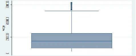
Outliers is an observation from a different population to that generating the remaining sample observations. The inclusion or exclusion of such an observation, especially if the sample size is small, can substantially alter the results of regression analysis. In Figure 1, the dots at top of the boxplot which indicates possible outliers, that is, these data points are more than 1.5 quartile (interquartile range) above the 75th percentile. The boxplot also confirm that the data is skewed to the right. Figure 2 shows the added variable plots, regressing each variable against all others, we noticed the coefficients on each. All the data points seem not to be in range, suggesting the presence of outliers. The consequence of this is that we cannot apply ordinary least squares regression model (OLS) on our raw data because of the BLUE (Best Linear Unbiased Estimator) which OLS tends to follow.
Figure 1: The Boxplot of FUTA Monthly Wage Distribution
Figure 2: The Added-variable Plot of FUTA Monthly Wage Distribution
b. SYMMETRY
A symmetry plot graphs the distance above the median for the i-th value against the distance below the median for the i-th value. A variable that is symmetric would have points that lie on the diagonal line. As we can see in figure 3, this distribution is not symmetric. Figure 4 is a Histogram with kernel density plot that produces a kind of histogram for the residual, the option normal overlays a normal distribution to Compare. Here residual seem not to follow a normal distribution and it is skewed to the right.
Figure 4: The Histogram with Kernel Density Plot of FUTA Monthly Wage Distribution
c. HOMOSCEDASTICITY
The error term ε is homoscedastic or equally spread, if the variance of the conditional distribution of εi given Xi, var (ε |
Xi ), is constant for i= 1…n and in particular does not depend
on X ; otherwise, the error term is heteroscedastic i.e differing variance (Stock and Watson, 2003). Depending on the nature of the heteroscedasticity, significance tests can be too high or too low. In addition, the standard errors are biased when heteroscedasticity is present. This in turn leads to bias in test statistics and confidence intervals.
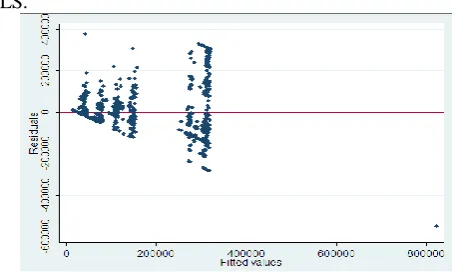
We plotted residuals against predicted values, using Stata SE, as shown in figure 5 we also used Breusch-Pagan test, a non-graphical method, to detect the presence of heteroscedasticity as shown in figure 6. The null hypothesis is that residuals are homoscedastic. We reject the null hypothesis at 95% and concluded that the residuals are not homogeneous.
Page 87 www.ijiras.com | Email: [email protected] this is that we may have the wrong estimates of the standard
errors for the coefficients and hence their p-value if we use OLS.
Figure 5: The scatterplot between residual and predicted values for Estimate of FUTA Monthly Wage Distribution
Figure 6: The Breusch-pagan and Vif tests
d. MULTICOLLINEARITY
An important assumption for the multiple regression model is that independent variables are not perfectly multicollinear. One regressor should not be a linear function of another. When multicollinearity is present standard errors may be inflated. Stata will drop one of the variables to avoid a division by Zero in the OLS procedure (Stock and Watson, 2003). In figure 7, all values of the variance inflation factor (VIF) are less than 10 suggest no multicollinearity. It is now evident from above sections that the data here is not normal and that no effect of multicollinearity. That no variable exhibit feature of normality. Therefore, estimation technique like ordinary least squares (OLS) will be biased, consequently the use of quantile regression estimation is more appropriate.
Quantile regression is a robust regression technique that accounts for the non-normal distribution of error terms and heteroscedasticity (Koenker and Bassett 1978; Koenker and Hallock 2001).
Unlike traditional linear models, such as OLS regression, that assume that estimates have a constant effect, quantile regression can illustrate if independent variables have non-constant or variable effects across the full distribution of the dependent variable. Standard errors for these quantile regression coefficient estimates were also obtained with bootstrapping method as shown in table1. This method
provides robust result (Kronecker and Hallock 2001), with the bootstrap method preferred to asymptotic method in terms of practicality (Hao and Maiman, 2007)
B. RESEARCH METHODOLOGY
The technique of estimation using Quantile Regression is applied to our dataset to our which is a sample of 1111 workers in the Federal University of Technology, Akure, Nigeria.
Standard least squares regression techniques provides summary point estimates that calculate the average effect of the independent variables on the wages of workers. We computed several regression curves corresponding to the various percentage points of the distributions and thus get a more complete picture of the set. Ordinarily this is not done, and so regression often gives a rather incomplete picture. Just as the mean gives an incomplete picture of a single distribution, so the regression curve gives a correspondingly incomplete picture for a set of distributions.
In the context of this study, all determinants of wage of workers is of interest in their own right, we don't want to dismiss them as outliers, but on the contrary we believe it would be worthwhile to study them in detail. This was done by calculating coefficient estimates at various quantiles of the conditional distribution using quantile regression approach which avoids the restrictive assumption that the error terms are identically distributed at all points of the conditional distribution. Relaxing this assumption allow us to acknowledge wages heterogeneity and consider the possibility that estimated slope parameters vary at different quantiles of the conditional distribution of wages. We then analyze the data by assuming that wage is the function of Age (year), sex, level of education and job tenure, which can be in:
Ordinary least square equations of the form:
Wagei = β0 + β1Agei + β2Sexi+ β3Edu2i+ β3Edu3i +
β4Edu3i + β5Jobti + εi (1)
Linear Quantile model of the form:
Wageθ, i = βθ,0 + βθ,1Agei + βθ,2Sexi+ βθ,3Edu2i+ βθ,4Edu3i +
βθ,5Jobti + εθ,i (2)
The variables are defined as follows: Wage = Monthly Wage income in Naira Age = Age in Years
Sex = An indicator variable using 1 to represent Male workers
and 0 to represent Female workers
Edu2 = An indicator variable using value 1 to represent workers who are graduates and 0 for workers who are not graduates
Edu3 = An indicator variable using value 1 to represent workers who have post graduate qualifications and 0 for workers without postgraduate qualifications.
Jobt = An indicator variable taking a value 1 for workers with Permanent Jobs and value 0 for workers with temporary jobs.
Page 88 www.ijiras.com | Email: [email protected] θ ε (0.05; 0.25; 0.5;0.75;0.95). We design our models as
shown below;
Wage0.05, i= β0.05,0 + β0.05,1Agei + β0.05,2Sexi+ β0.05,3Edu2i+
β0.05,4Edu3i + β0.05,5Jobti + ε0.05,i (3)
Wage0.25, i= β0.25,0 + β0.25,1Agei + β0.25,2Sexi+ β0.25,3Edu2i+
β0.25,4Edu3i + β0.25,5Jobti + ε0.25,i (4)
Wage0.5, i = β0.5,0 + β0.5,1Agei + β0.5,2Sexi+ β0.5,3Edu2i+
β0.5,4Edu3i + β0.5,5Jobti + ε0.5,i (5)
Wage0.75, i= β0.75,0 + β0.75,1Agei + β0.75,2Sexi+ β0.75,3Edu2i+
β0.75,4Edu3i + β0.75,5Jobti + ε0.75,i (6)
Wage0.95, i= β0.95,0 + β0.95,1Agei + β0.95,2Sexi+ β0.95,3Edu2i+
β0.95,4Edu3i + β0.95,5Jobti + ε0.95,i (7)
We solved equations (3), (4), (5), (6), (7) using sqreg module of STATA SE for simultaneous quantile regression estimation and obtained an estimate of the entire variance-covariance of the estimates by bootstrapping with 100 bootstrap replication. We also obtain ordinary least square model from the equations (1) using Gretl package.
IV. DISCUSSION OF RESULTS
Table 1 is the result obtained when we solved equations (3) through (7) using Sgreg module of STATA SE for simultaneous quantile regression with 100 bootstrap replication. We also obtained ordinary least square model from the equation (1) using Gretl package as shown in the last column Table 2 is the result obtained when we tested the equivalence of coefficient across quantiles using STATA SE. We used Gretl package to obtain figures 7 to 11, they illustrate how the effects of wage distribution vary over quantiles, and how the magnitude of the effects at various quantiles differ considerably from the OLS coefficient, even in terms of the confidence intervals around each coefficient.
Table 1: Model of FUTA Monthly Income via OLS with 100 Resampling Bootstrap
In table 1, the bootstrap standard error of estimate with 100 replication are shown in brackets. We then used bootstrap standard error in place of asymptotic standard error because the assumption of independent and identical distribution (i.i.d) did not hold in our data set. The bootstrap standard error of Age for 0.05th, 0.25th, 0.5th,0.75th, 0.95th and that of OLS are respectively 114, 568, 976, 1069, 560 and 3135 and the p-value for all coefficients, except that of 0.05th, 0.25th and OLS ,are less than 0.05 level of Significance providing evidence to reject the null hypothesis that Age has no effect on monthly earning at all quantiles. Similarly, the bootstrap standard error of sex for 0.05th, 0.25th , 0.5th,0.75th 0.95th and OLS are 650,1593,3461,8319,12750 and 10518 and the
p-value for coefficients and that of OLS are more than 0.05 with the exception of 0.75th quantile and OLS.
Also the bootstrap standard error of education variables, Edu2 and Edu3, for 0.05th, 0.25th , 0.5th,0.75th and 0.95th are shown in table 1 and the p-value for all predictors on response variables are all less than 0.05 level of significance at all quantiles with the exception of 0.05th quantile.
Figure 7: The marginal Effects of Age for all Quantiles and OLS of the FUTA Monthly Wage.While the bootstrap
standard error of jobt for 0.05th, 0.25th, 0.5th,0.75th,0.95th
and OLS are 1304,2019,14342,14824,12725 and 24107 and the p-value for coefficients are more than 0.05 with the
exception of 0.25th and 0.75th
Figure 8: The Marginal Effects of Sex for all Quantiles and OLS of the FUTA Monthly Wage
Looking at the coefficient estimates that quantile regression and OLS provide us with in table 1, one finds out that:
AT LOWER TAIL (I.E AT LEFT TAIL) OF A DISTRIBUTION
For 0.05th quantile, all predictor variables are not significant. That is only intercept is not significant with positive coefficient. However, in case of 0.25th quantile, only Age and sex and the intercept are not significant with positive coefficient and Edu2,Edu3 job tenure are significant with positive coefficient.
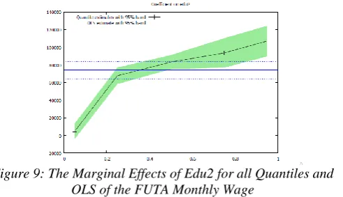
Figure 9: The Marginal Effects of Edu2 for all Quantiles and OLS of the FUTA Monthly Wage
CHAR 0.05Q 0.25Q 0.50Q 0.75Q 0.95Q OLS
Intercept 18526 [5892] (0.0020) 2106.94 [0.9360] (0.9360) -65053.4 [34038] (0.0590) -134000 [38725] (0.0010) -130870 [22899] (0.0000) -1570.93 [1246] (0.990) Age 117.90
(114) (0.3030) 494.64 [568] (0.3840) 2434.12 [976] (0.0130) 5431.33 [1069] (0.0000) 5823.13 [560] (0.0000) 508.59 [3135] (0.8710) Sex 117.90
[650] (0.8560) 1382.69 [1593] (0.3930) 4699.16 [3461] (0.1750) 16947.4 [8319] (0.0420) 14865.4 [12750] (0.2440) 34579.60 [10518] (0.0010) Edu2 4330.11
[8548] (0.6130) 67647.5 [4305] (0.0000) 83161.6 [5567] (0.0000) 93529.7 [8151] (0.0000) 107070 [11089] (0.0000) 73941.36 [14474] (0.0000) Edu3 10047.8
Page 89 www.ijiras.com | Email: [email protected] AT MIDDLE TAIL (I.E AT MEDIAN) OF A
DISTRIBUTION TAIL
For OLS, it rely on the property of BLUE. i.e among all the unbiased estimators, OLS does not provide the estimate with the smallest variance. It is the best linear unbiased estimator, if the following four assumptions hold.
The explanatory variable xi is non-stochastic
The expectation variable of the error term εi are zero i.e
E(εi) = 0
Homoscedasticity. the variance of the error εi is constant
i.e Var (εi)= ϭ2
No autocorrelation. i.e Cov (εi, εj =0) i≠j
Figure 10: The Marginal Effects of Edu3 for all Quantiles and OLS of the FUTA Monthly Wage
Hence, the results obtained by OLS in the last column in table 1 is bias and distorted because of the properties of BLUE which our data fail to follow.
A more comprehensive picture of the effect of Age, Sex, Edu2, Edu3 and Jobt on the monthly wage are obtained by using median Quantile Regression as shown in the third column in table 1.
Median QR can be used in place of OLS because both attempt to model the central location of a response-variable distribution. Where we want to understand the central tendency in a data set, OLS loses its effectiveness whenever it attempts to go towards the extremes of a data set. Because of the property of BLUE which it holds on.
Figure 11: The Marginal Effects of Jobt for all Quantiles and OLS of the FUTA Monthly Wage
For 0.5th quantile (median quantile)Age, Edu2 and Edu3 are significant with positive coefficient and Sex, and Jobt are not at all significant.
AT UPPER TAIL (I.E AT RIGHT TAIL) OF A DISTRIBUTION
for 0.75th quantile, Age, sex, Edu2 and Edu3 are significant with positive coefficient and Jobt are significant with negative coefficient.
for highest quantile, 0.95th quantile, results are similar to the case of 0.5th quantile but its effect are stronger than that of 0.5th quantile.
Figures 4.7 to 4.11 show the marginal effects of
all variables Age ,Sex, Edu2, Edu3 and Jobt for all quantiles within the (0, 1) range of the monthly wage. The horizontal lines (solid line) refer to the OLS coefficient and the difference between the OLS and the marginal effects of Age ,Sex, Edu2, Edu3 and Jobt for all percentage points of the quantiles in the monthly wage help us to understand how changing this effect can be. It is also apparent that the slope of the regression changes across the quantiles and is clearly not constant, as presumed by OLS. They also highlight that a linear regression might not be an optimum solution to assess the relationship between monthly wage and Age, Sex, Edu2, Edu3 and Jobt in the conditional mean model.
V. CONCLUSION AND RECOMMENDATION
In this chapter, a general conclusion and recommendation on this research work were made. The study was intended to identify the effect of Age, Education and Job tenure on monthly wage distribution.
A. CONCLUSION
The dependent variable showed skewed distribution, this study therefore, relies on quantile regression analysis. Stata and Gretl packages were used for the implementation of quantile regression. The quantile θ values considered are 0.05, 0.25, 0.50, 0.75and 0.95. Results showed that for all quantile, wage is positively related to Age, gender, graduated and post graduated workers. However, wage is negatively related to job permanency only at the middle and higher quantiles but positively related to wage at lower quantiles but not statistically significant.
The coefficient of age shows that an additional year produces positive effect on monthly wage of workers for all quantiles and OLS but not statistically significant at lower quantiles and OLS. A worker earns more money at median quantile and OLS than at lower quantile, but earns less at median quantile and OLS than higher quantile.
Page 90 www.ijiras.com | Email: [email protected] 0.75 and 0,95th quantiles) than worker whose job are
temporary. Also coefficient of the sex variable for all quantiles and OLS suggest that male workers earns more wage than female workers at all quantiles but not statistically significant except at 0.75th quantile. These show that education disequilibrium, age, gender difference and job tenure produce significant effect on monthly wage differential of workers.
B. RECOMMENDATION
The results shown in the last column in table 1 reveal that ordinary least square approach is inadequate for a variety of reasons, including the presence of heteroscedasticity, outliers etc and the failure to detect multiple form of shape shift. These defects are not restricted to the study of wage disparity alone but also appear when other measures are considered. Therefore, it is recommended to have an alternative in the form of quantile regression approach that is built to handle heteroscedasticity and outliers and that will be able to detect various forms of shape changes.
Thus, the use of Quantile Regression as an alternative to Ordinary Least Squares Regression in analyzing wages inequality is therefore recommended for use not only in econometrics, but also in finance, biomedicine, data mining, and environmental studies.
REFERENCES
[1] Abadie A., Angrist J.and Imbens, G., (2002), Instrumental Variables Estimates of the Effect of Subsidized Training on the Quantiles of Trainee Earnings Econometrica 70, page 91-117.
[2] Abreveya J.(2001), The Effects of Demographics and Maternal Behavior on the Distribution of Birth Outcomes Empirical Economics, 26, page 247-257.
[3] Antonella C., (2015), The Effect of M@tabel on Italian Students' A Quantile Regression Approach 7th World Conferene on Educational Sciences. (WCES-2015). www.Sciencedirect.com.
[4] Aviral K.T and Raveesh K., (2015), Determinant of Capital Structure: A Quantile Regression Analysis Studies in Business and Economics no 10(1) 2015, page 16 - 34. [5] Buchinsky M., (1994), Changes in the U.S. Wage
Structure Application of Quantile Regression Econometrica, 62, page 405-458.
[6] Budd J. W. & McCall B. P., (2001), The Grocery Stores Wage Distribution: A Semi Parametric Analysis of the Role of Retailing and Labor Market Institutions Industrial and Labor Relations Review, 54, Extra Issue: Industry Studies of Wage Inequality, page 484-501
[7] Budria S. and Moro-Egido A.I., (2008), Education, Educational Mismatch and Wage Inequality: Evidence for Spain Economics of Education Review, 27(3), page 332-341.
[8] Budra S. and Pereira P.T., (2005), Educational Qualifications on Wage Inequality: Evidence for Europe IZA Discussion Paper No. 1763.
[9] Cade B. S., Terrell J. W.& Schroeder R. L., (1999), Estimating Effects of Limiting Factors with Regression Quantiles Ecology, 80, page 311-323.
[10]Chay K. Y. & Honore B. E., (1998), Estimation of Semi parametric Censored Regression Models: An Application to Changes in Black-White Earnings Inequality during the 1960s The Journal of Human Resources, 33, page 438. [11]Chamberlain G., (1994), Quantile Regression, Censoring
and the Structure of Wages InC. Skins (Ed.), Advances in Econometrics (page 171-209). Cambridge, UK: Cambridge University Press.
[12]Eide E. R. & Showalter M. H., (1999), Factors Affecting the Transmission of Earnings across Generations: A Quantile Regression Approach. The Journal of Human Resources, 34, page 253-267.
[13]Eide E. R., Showalter M. & Sims D., (2002), The Effects of Secondary School Quality on the Distribution of Earnings Contemporary Economic Policy, 20, page 160-170.
[14]Falaris E. M., (2008), A Quantile Regression Analysis is of Wages in Panama Review of Development Economics, 12 (3) page 498-514.
[15]Girma S. and Kedir A., (2003), Is Education More Beneficial to the Less Able? Econometric Evidence from Ethiopia Department of Economics, Working Paper No: 03/1. University of Leicester, UK.
[16]Grazyna T., (2011), Some Test for Quantile Regression Model Acta universitatis Lodzienis Folia Oeconomica 255, page 125 - 135.
[17]Hartog J., Pereira P., Vieira J.C., (2001), Changing Returns to Education in Portugal during the 1980s and early 1990s: OLSR and Quantile Regression Estimators Applied Economics 33,page 1021-1037.
[18]Machado J. F. and Mata J., (2005), Counterfactual Decomposition of Changes in Wage Distributions using Quantile Regression Journal of Applied Econometrics, 20(4), page 445-465.
[19]Martins P.S and Pereira P.T., (2004), Does Education Reduce Wage Inequality? Quantile Regressions Evidence from Fifteen European Countries Labour Economics,11 (3), page 535-571.
[20]Pereira P.T and P.S. Martins., (2002), Is there a Return-Risk Link in Education? Economics Letters,75, page 317. [21]Martins P.S and Pereira P.T., (2004), Does Education
Reduce Wage Inequality? Quantile Regressions Evidence from Fifteen European Countries Labour Economics,11 (3), page 535-571.
[22]Prieto R., Barros C.P. and Vieira J. A. C. (2008), What a Quantile Approach can Tell Us about Returns to Education in Europe Education Economics, 16(4) page 391-410.
[23]Lemieux T., (2007), The Changing Nature of Wage Inequality Cambridge, MA: National Bureau of Economic Research (NBER) Working Paper No: 13523.
Page 91 www.ijiras.com | Email: [email protected] [25]Machado J. F. and Mata J., (2005), Counterfactual
Decomposition of Changes in Wage Distributions using Quantile Regression Journal of Applied Econometrics, 20(4), page 445-465.
[26]Fortin N. M. & Lemieux T., (1998), Rank Regressions, Wage Distributions, and the Gender Gap The Journal of Human Resources, 33, page 610-643.., (2005), Immigration and Wealth Inequality: A Distributional Approach Invited Seminar at The Center for the Study of Wealth and Inequality, Columbia University.
[27]Hao L., (2006), Sources of Wealth Inequality: Analyzing conditional distribution Invited Seminar at The Center for Advanced Social Science Research, New York University. [28]Hao L. and Naima D.Q., (2007), Quantile Regression
Thousand Oaks, Calif: Sage Publication.
[29]Koenker Koenker R.and Basset G., (1978), Regression Quantile Economica, 46, page 33-50.
[30]Koenker R. and Hallock K., (2001), Quantile Regression: An introduction Journal of Economic perspective, 15, page 143- 156.
[31]Lemieux T., (2006), Post-Secondary Education and Increasing Wage Inequality Working Paper No. 12077. Cambridge, MA: National Bureau of Economic Research. [32]Scharf F. S., Juanes F. & Sutherland M. (1989), Inferring Ecological Relationships from the edges of [21] Scatter Diagrams: Comparison of Regression Techniques Ecology, 79, page 448-460.
[33]Ramsey J.B., (1969), Test for Specification Errors in Classical Linear Least-Squares Regression Analysis J.R. Stat. soc B. 31 page 356-371.