e-ISSN: 2278-7461, p-ISSN: 2319-6491
Volume 5 Issue 8 [Sep2016] PP: 61-71
Collocation Method for Seventh Order Boundary Value
Problems Using Quintic B-Splines
S. M. Reddy
Department of Science and Humanities, Sreenidhi Institute of Science and Technology, Hyderabd-India-501 301
Abstract
:
A finite element method involving collocation method with quintic B-splines as basis functions has been developed to solve seventh order boundary value problems. The seventh, six and fifth order derivatives for the dependent variable is approximated by the finite differences. The basis functions are redefined into a new set of basis functions which in number match with the number of collocated points selected in the space variable domain. The proposed method is tested on three linear and two non-linear boundary value problems. The solution to a nonlinear problem has been obtained as the limit of a sequence of solutions of linear problems generated by the quasilinearization technique. Numerical results obtained by the present method are in good agreement with the exact solutions available in the literature.Keywords: Collocation method, Quintic B-spline, Seventh order boundary value problem, Absolute error.
I.
INTRODUCTION
In this paper, we consider a general seventh order boundary value problem
( 7 ) ( 6 ) ( 5 ) ( 4 )
5
0 1 2 3 4
6 7
( ) ( ) ( ) ( ) ( ) ( ) ( ) ( ) ( ) ( ) ( ) ( )
( ) ( ) ( ) ( ) ( ) ,
a x y x a x y x a x y x a x y x a x y x a x y x
a x y x a x y x b x c x d
(1)
subject to boundary conditions
0 0 1 1 2 2 3
( ) , ( ) , ( ) , ( ) , ( ) , ( ) , ( )
y c A y d C y c A y d C y c A y d C y c A (2) where A0, C0, A1, C1, A2, C2, A3 are finite real constants and a0(x), a1(x), a2(x), a3(x), a4(x), a5(x), a6(x), a7(x) and b(x) are all continuous functions defined on the interval [c, d].
In this paper, we try to present a simple finite element method which involves collocation approach with quintic B-splines as basis functions to solve the seventh order boundary value problem of the type (1)-(2). This paper is organized as follows. In section II of this paper, the justification for using the collocation method has been mentioned. In section III, the definition of quintic B-splines has been described. In section IV, description of the collocation method with quintic B-splines as basis functions has been presented and in section V, solution procedure to find the nodal parameters is presented. In section VI, numerical examples of both linear and non-linear boundary value problems are presented. The solution to a nonnon-linear problem has been obtained as the limit of a sequence of solution of linear problems generated by the quasilinearization technique [2]. Finally, the last section is dealt with conclusions of the paper.
II.
JUSTIFICATION
FOR
USING
COLLOCATION
METHOD
In finite element method (FEM) the approximate solution can be written as a linear combination of basis functions which constitute a basis for the approximation space under consideration. FEM involves variational methods like Ritzs approach, Galerkins approach, least squares method and collocation method etc. The collocation method seeks an approximate solution by requiring the residual of the differential equation to be identically zero at N selected points in the given space variable domain where N is the number of basis functions in the basis [6]. That means, to get an accurate solution by the collocation method one needs a set of basis functions which in number match with the number of collocation points selected in the given space variable domain. Further, the collocation method is the easiest to implement among the variational methods of FEM. When a differential equation is approximated by mth order B-splines, it yields (m + 1)th order accurate results [8]. Hence this motivated us to solve a seventh order boundary value problem of type (1)-(2) by collocation method with quintic B-splines as basis functions.
III.
DEFINITION
OF
QUINTIC
B-SPLINES
The quintic B-splines are defined in [3, 8, 9]. The existence of quintic spline interpolate s(x) to a function in a closed interval [c, d] for spaced knots (need not be evenly spaced) of a partition c = x0 < x1 <…< xn-1 < xn= d
is established by constructing it. The construction of s(x) is done with the help of the quintic B-splines. Introduce ten additional knots x-5, x-4, x-3, x-2, x-1, xn+1, xn+2, xn+3, xn+4 and xn+5 in such a way that
x-5<x-4<x-3<x-2<x-1<x0 and xn<xn+1<xn+2<xn+3<xn+4< xn+5.
Now the quintic B-splines Bi(x)'s are defined by
5 3
3 3
3
( )
, [ , ]
( ) ( )
0 ,
i r
i i r i
i r
x x
x x x
B x x
o t h e r w i s e
where
5
3 ( ) ,
( )
0 ,
r r
r
r
x x if x x
x x
if x x
and
3
3
( ) ( )
i
r r i
x x x
where {B-2(x), B-1(x), B0(x), B1(x),…,Bn(x), Bn+1(x), Bn+2(x)} forms a basis for the spaces5() of quintic
polynomial splines. Schoenberg [9] has proved that quintic B-splines are the unique nonzero splines of smallest compact support with the knots at
x-5<x-4<x-3<x-2<x-1<x0<x1<…<xn-1<xn<xn+1<xn+2<xn+3<xn+4< xn+5.
IV.
D
ESCRIPTION OF THE METHODTo solve the boundary value problem (1) subject to boundary conditions (2) by the collocation method with quintic B-splines as basis functions, we define the approximation for y x( ) as
2
2
( ) ( )
n
j j j
y x B x
(3)Where j's are the nodal parameters to be determined and Bj( ) 'x s are quintic B-spline basis functions. In
the present method, the mesh points
3 2, 3, ...., n , n 1
method, the number of basis functions in the approximation should match with the number of collocation points [6]. Here the number of basis functions in the approximation (3) is n+5, where as the number of selected collocation points is n-2. So, there is a need to redefine the basis functions into a new set of basis functions which in number match with the number of selected collocation points. The procedure for redefining the basis functions is as follows:
Using the definition of quintic B-splines, the Dirichlet, Neumann, second order derivatives boundary conditions and third order derivative boundary condition of (2), we get the approximate solution at the boundary points as
2
0 0 0
2
( ) ( ) j j( )
j
y c y x
B x A
(4)2
0 2
( ) ( ) ( )
n
n j j n
j n
y d y x
B x C
(5)2
0 0 1
2
( )
(
)
j j(
)
j
y
c
y
x
B
x
A
(6)2
1 2
( ) ( ) ( )
n
n j j n
j n
y d y x
B x C
(7)2
0 0 2
2
( ) ( ) j j( )
j
y c y x
B x A
(8)2
2 2
(
)
(
)
j j(
)
j
n n
y
d
y
x
B
x
C
(9)2
3
0 0
2
( ) ( ) j j ( )
j
y c y x
B x A
(10)Eliminating 2,1, 0, 1, n, n1 and
n2 from the equations (3) to (10), we get the approximation for y(x) as1
2
( )
( )
( )
n
j j
j
y x
w x
S
x
(11)where
3 3 0 1 0 1 3
( )
( ) ( ) ( )
( )
w x A
w x w x R x
R x
2 2 2 2
3 2 0
0 0 0
( ) ( )
( ) ( ) ( ) ( )
( ) ( n) n
n n
A C
w x w x w x Q w x
Q
x Q x
Q
x x
1 1 0 1 1
2 1
1
1 1
0 1
( ) ( ) ( ) ( )
( ) ( )
( ) ( )
n n
n n
A C
w x w x w x P x w x P x
x
P P x
0 0
1 2 2
2 0 2
( ) ( ) ( )
( ) n ( n) n
A C
w x B x B x
B x B x
0 1 1 0
( )
( ) ( ) , 2
( )
( )
( ) , 3 , 4 , ..., 1
j j
j
j
R x
R x R x j
R x
S x
R x j n
(12) 0 0 0 0 ( )
( ) ( ) , 1, 2
( )
( ) ( ) , 3 , 4 , ..., 3
( )
( ) ( ) , 2 , 1
( ) j j j j j n j n n n Q x
Q x Q x j
Q x
R x Q x j n
Q x
Q x Q x j n n
Q x 0 1 1 0 1 1 ( )
( ) ( ) , 0 , 1, 2
( )
( ) ( ) , 3 , 4 , ..., 3
( )
( ) ( ) , 2 , 1,
( ) j j j j j n j n n n P x
P x P x j
P x
Q x P x j n
P x
P x P x j n n n
P x 0 2 2 0 2 2 ( )
( ) ( ) , 1, 0 , 1, 2
( )
( ) ( ) , 3 , 4 , ..., 3
( )
( ) ( ) , 2 , 1, , 1
( ) j j j j j n j n n n B x
B x B x j
B x
P x B x j n
B x
B x B x j n n n n
B x
Now the new basis functions for the approximation y(x) are {Sj(x), j=2, 3,…, n-1} and they are in
number match with the number of selected collocated points. Since the approximation for y(x) in (11) is a quintic approximation, let us approximate y(5), y(6) and y(7) at the selected collocation points with finite differences as
( 4 ) ( 4 )
( 5 ) 1 1
f o r
2 , 3, ...,
1
2
i i
i
y
y
y
i
n
h
(13)( 4 ) ( 4 ) ( 4 ) ( 6 ) 1 1
2
2
f o r 2 , 3, ...., 1
i i i i
y y y
y i n
h
(14)
( 4 ) ( 4 ) ( 4 ) ( 4 ) ( 7 ) 2 1 1 2
3
2 2
f o r 2 , 3, ...., 2 2
i i i i i
y y y y
y i n
h
(15)
( 4 ) ( 4 ) ( 4 ) ( 4 )
( 7 ) 1 2 3
3
3 3
f o r 1
i i i i
i
y y y y
y i n
h
(16)
1
2
( ) ( ) ( )
n
i i i j j i j
y y x w x S x
(17)Now applying the collocation method to (1), we get
( 7 ) ( 6 ) ( 5 ) (
2 3
4 )
4 5
0 1 6
7
( ) ( ) ( ) ( ) ( ) ( ) ( )
( ) ( ) f o r 2 , 3 , , 1 .
i i i i i i i i i i i i i i i i i
a x y a x y a x y a x y a x y a x y a x y
a x y b x i n
(18)
Substituting (13) to (17) in (18), we get
1 1 1
( 4 ) ( 4 ) ( 4 ) ( 4 ) ( 4 ) ( 4 ) ( 4 )
2 2 1 1 1 1 2
2 2 2
0
3 1
( 4 ) 2 2
1
( 4 ) ( 4 ) ( 4 )
1
1 1
2
2
( ) ( ) 2 ( ) 2 ( ) 2 ( ) ( ) ( )
( ) 2
( )
( )
( ) ( ) 2 ( )
n n n
i j j i i j j i i j j i i
j j j
i n
j j i j
n i
i j j i i
j
w x S x w x S x w x S x w x
a x
h
S x
a x
w x S x w x
h
1 1( 4 ) ( 4 ) ( 4 )
1 1
2 2
1 1
( 4 ) ( 4 ) ( 4 ) ( 4 )
2
1 1 1 1
2 2
1
( 4 ) ( 4 )
3 4
2
2 ( ) ( ) ( )
( )
( ) ( ) ( ) ( )
2
( ) ( ) ( ) ( ) ( )
n n
j j i i j j i
j j
n n
i
i j j i i j j i
j j
n
i i j j i i i j j
j j
S x w x S x
a x
w x S x w x S x
h
a x w x S x a x w x S
1 5 12 2 1 1 6 7 2 2 ( ) ( ) ( ) ( ) ( ) ( ) ( ) ( ) ( ) ( ) n n
i i i j j i
j
n n
i i j j i i i j j i
j j
x a x w x S x
a x w x S x a x w x S x
for i=2, 3,…, n-2. (19)
1 1 1
( 4 ) ( 4 ) ( 4 ) ( 4 ) ( 4 ) ( 4 ) ( 4 )
1 1 2 2 3
2 2 2
0
3 1
( 4 ) 3 2
1
( 4 ) ( 4 ) ( 4 )
1
1 1
2
2
( ) ( ) 3 ( ) 3 ( ) 3 ( ) ( ) ( )
( )
( )
( )
( ) ( ) 2 ( ) 2
n n n
i j j i i j j i i j j i i
j j j
i n
j j i j
n i
i j j i i j
j
w x S x w x S x w x S x w x
a x
h
S x
a x
w x S x w x S
h
1 ( 4 ) ( 4 ) 1 ( 4 )1 1
2 2
1 1
( 4 ) ( 4 ) ( 4 ) ( 4 )
2
1 1 1 1
2 2
1 1
( 4 ) ( 4 )
3 4 2 2 ( ) ( ) ( ) ( ) ( ) ( ) ( ) ( ) 2 ( ) ( ) ( ) ( ) ( ) n n
j i i j j i
j j
n n
i
i j j i i j j i
j j
n n
i i j j i i i j j
j j
x w x S x
a x
w x S x w x S x
h
a x w x S x a x w x S
5 12 1 1 6 7 2 2 ( ) ( ) ( ) ( ) ( ) ( ) ( ) ( ) ( ) ( ) n
i i i j j i
j
n n
i i j j i i i j j i
j j
x a x w x S x
a x w x S x a x w x S x
for i=n-1. (20)
Rearranging the terms and writing the system of equations (19) and (20) in matrix form, we get
A B (21)
where A [ai j] ;
( 4 ) ( 4 ) ( 4 ) ( 4 ) ( 4 ) ( 4 ) ( 4 )
0 1
2 1 1 2 1
3 2
( 4 ) ( 4 ) ( 4 ) ( 4 )
1
1 2 3 4 5
( ) ( )
( ) 2 ( ) 2 ( ) ( ) ( ) 2 ( ) ( )
2
( )
( ) ( ) ( ) ( ) ( ) ( ) ( ) ( ) ( ) 2
i i
i j j i j i j i j i j i j i j i
i
j i j i i j i i j i i j i i
a x a x
a S x S x S x S x S x S x S x
h h
a x
S x S x a x S x a x S x a x S x a x
h
6 7
( )
( ) ( ) ( ) ( )
j i
i j i i j i
S x
a x S x a x S x
for i= 2, 3 …., n-2; j=2, 3,…, n-1. (22)
( 4 ) ( 4 ) ( 4 ) ( 4 ) ( 4 ) ( 4 ) ( 4 )
0 1
1 2 3 1
3 2
( 4 ) ( 4 ) ( 4 ) ( 4 )
1
1 2 3 4 5
( ) ( )
( ) 3 ( ) 3 ( ) ( ) ( ) 2 ( ) ( )
( )
( ) ( ) ( ) ( ) ( ) ( ) ( ) ( ) ( ) 2
i i
i j j i j i j i j i j i j i j i
i
j i j i i j i i j i i j i i
a x a x
a S x S x S x S x S x S x S x
h h
a x
S x S x a x S x a x S x a x S x a x S
h
6 7
( )
( ) ( ) ( ) ( )
j i
i j i i j i
x
a x S x a x S x
for i= n-1; j=2, 3,…, n-1. (23)
[bi] ;
B
( 4 ) ( 4 ) ( 4 ) ( 4 ) ( 4 ) ( 4 ) ( 4 )
0 1
2 1 1 1 1 1
3 2
( 4 ) ( 4 ) ( 4 )
2
1 1 3 4 5
6 7
( ) ( )
( ) 2 ( ) 2 ( ) ( ) ( ) 2 ( ) ( )
2
( )
( ) ( ) ( ) ( ) ( ) ( ) ( ) ( ) 2
( ) ( ) (
i i
i i i i i i i i
i
i i i i i i i i
i i
a x a x
b w x w x w x w x w x w x w x
h h
a x
w x w x a x w x a x w x a x w x
h
a x w x a
xi)w x( i)
for i= 2, 3, …, n-2. (24)
( 4 ) ( 4 ) ( 4 ) ( 4 ) ( 4 ) ( 4 ) ( 4 )
0 1
1 2 3 1 1
3 2
( 4 ) ( 4 ) ( 4 )
2
1 1 3 4 5
6 7
( ) ( )
( ) 3 ( ) 3 ( ) ( ) ( ) 2 ( ) ( )
( )
( ) ( ) ( ) ( ) ( ) ( ) ( ) ( )
2
( ) ( ) ( )
i i
i i i i i i i i
i
i i i i i i i i
i i i
a x a x
b w x w x w x w x w x w x w x
h h
a x
w x w x a x w x a x w x a x w x
h
a x w x a x
w x( i)
for i= n-1. (25)
and [2,3,,n1] .T
V.
SOLUTION
PROCEDURE
TO
FIND
THE
NODAL
PARAMETERS
equations (21) is a ten band system ini's. The nodal parameters i 's can be obtained by using band matrix solution package. We have used the FORTRAN-90 programming to solve the boundary value problem (1)-(2) by the proposed method.
VI.
NUMERICAL
RESULTS
To demonstrate the applicability of the proposed method for solving the seventh order boundary value problems of the type (1) and (2), we considered three linear and two nonlinear boundary value problems. The obtained numerical results for each problem are presented in tabular forms and compared with the exact solutions available in the literature.
Example 1: Consider the linear boundary value problem
( 7 ) 2
(3 5 1 2 1 2 ) x, 0 1
y y x x e x (26) subject to
( 0 ) 0 , (1) 0 , ( 0 ) 1, (1) , ( 0 ) 0 , (1) 4 , ( 0 ) 3 .
y y y y e y y e y
The exact solution for the above problem is y x(1 x e) x.
The proposed method is tested on this problem where the domain [0, 1] is divided into 10 equal subintervals. The obtained numerical results for this problem are given in Table 1. The maximum absolute error obtained by the proposed method is 3 .0 6 9 6 3 91 06.
Table 1: Numerical results for Example 1
Example 2: Consider the linear boundary value problem
( 7 ) 2
( 2 6 ) x, 0 1
y x y x x e x (27) subject to
( 0 ) 1, (1) 0 , ( 0 ) 0 , (1) , ( 0 ) 1, (1) 2 , ( 0 ) 2 .
y y y y e y y e y
The exact solution for the above problem is y ex(x1).
The proposed method is tested on this problem where the domain [0, 1] is divided into 10 equal subintervals. The obtained numerical results for this problem are given in Table 2. The maximum absolute error obtained by the proposed method is 1 .5 8 5 4 8 41 05.
x
Absolute error by the proposed method
0.1 1.862645E-07
0.2 1.490116E-08
0.3 8.642673E-07
0.4 1.698732E-06
0.5 2.831221E-06
0.6 3.069639E-06
0.7 1.549721E-06
0.8 4.172325E-07
Table 2: Numerical results for Example 2
Example 3: Consider the linear boundary value problem
( 7 ) ( 4 )
s in (1 ) ( 2 s in ) x, 0 1
y x y c o s x y x y xc o s xx e x (28)
subject to
( 0 ) 1, (1) , ( 0 ) 1, (1) , ( 0 ) 1, ( 0 ) .
y y e y y e y y e
The exact solution for the above problem is y ex.
The proposed method is tested on this problem where the domain [0, 1] is divided into 10 equal subintervals. The obtained numerical results for this problem are given in Table 3. The maximum absolute error obtained by the proposed method is 3 .0 8 7 5 2 11 05.
Table 3: Numerical results for Example 3
x
Absolute error by the proposed method
0.1 1.370907E-06
0.2 4.529953E-06
0.3 8.881092E-06
0.4 1.382828E-05
0.5 1.585484E-05
0.6 1.478195E-05
0.7 1.144409E-05
0.8 6.586313E-06
0.9 2.443790E-06
x
Absolute error by the proposed method
0.1 1.788139E-06
0.2 1.311302E-06
0.3 3.457069E-06
0.4 1.060963E-05
0.5 2.157688E-05
0.6 3.087521E-05
0.7 3.075600E-05
0.8 2.193451E-05
Example 4: Consider the nonlinear boundary value problem
( 7 ) 2 2
( 2 ( 8 ) 3 ), 0 1
x x
y y ye e x x x x (29)
subject to
1
1
( 0 ) 1, (1) 0 , ( 0 ) 2 , (1) ,
( 0 ) 3 , (1) 2 , ( 0 ) 4 .
y y y y e
y y e y
The exact solution for the above problem is y (1x e) x.
The nonlinear boundary value problem (29) is converted into a sequence of linear boundary value problems generated by quasilinearization technique [2] as
( 7 ) 2 2
( 1 ) ( ) ( 1 ) ( ) ( 1 ) ( 2 ( 8 ) 3 ) ( ) ( ), 0 , 1, 2 , ...
x x
n n n n n n n
y y y y y e e x x x y y n (30) Subject to
1 1
(n 1 )( 0 ) 1, (n 1 )(1) 0 , (n 1 )( 0 ) 2 , (n 1 ) (1) , (n 1 )( 0 ) 3 , (1)(n 1 ) 2 , (n 1 )( 0 ) 4 .
y y y y e y y e y
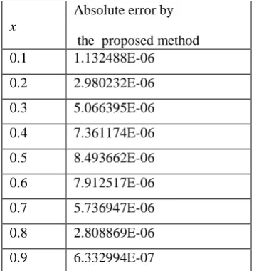
Here y(n1 ) is the (n1)th approximation for y x( ) . The domain [0, 1] is divided into 10 equal subintervals and the proposed method is applied to the sequence of linear problems (30). The obtained numerical results for this problem are presented in Table 4. The maximum absolute error obtained by the proposed method is 8.493662x10⁻⁶.
Table 4: Numerical results for Example 4
Example 5: Consider the nonlinear boundary value problem
( 7 ) ( 4 ) ( 1 )
( (1 2 4 ( 1) ) 8 ( 5 ) ) , 0 1
x
y x e x c o s x
y y e y e x e x c o s x x s i n x x (31) subject to
( 0 ) 1, (1) 0 , ( 0 ) 0 , (1) 1, ( 0 ) 2 , (1) 2 1 2 1, ( 0 ) 2 .
y y y y e c o s y y e c o s e s in y
The exact solution for the above problem is y ex(1x s in x) .
The nonlinear boundary value problem (31) is converted into a sequence of linear boundary value problems generated by quasilinearization technique [2] as
( )
( )
( 7 ) ( 4 ) ( 1 ) ) ( 1 ) ( 1 ) ( ) ( 1 )
2 ( )
(1 ) ( (1 2 4 ( 1)
8 ( 5 ) ) 0 , 1, 2 , ...
x n
n
y x e x c o s x
n n n n
y n
y y e y y e x e x c o s x
x s i n x e y n
(32)
subject to
( 1 ) ( 1 ) ( 1 ) ( 1 )
( 1 ) ( 1 ) ( 1 )
( 0 ) 1, (1) 0 , ( 0 ) 0 , (1) 1,
( 0 ) 2 , (1) 2 1 2 1, ( 0 ) 2 .
n n n n
n n n
y y y y e c o s
y y e c o s e s i n y
x
Absolute error by the proposed method
0.1 1.132488E-06
0.2 2.980232E-06
0.3 5.066395E-06
0.4 7.361174E-06
0.5 8.493662E-06
0.6 7.912517E-06
0.7 5.736947E-06
0.8 2.808869E-06
Here y(n1 ) is the (n1)th approximation for y x( ) . The domain [0, 1] is divided into 10 equal subintervals and the proposed method is applied to the sequence of linear problems (32). The obtained numerical results for this problem are presented in Table 5. The maximum absolute error obtained by the proposed method is 1.037121x10⁻⁵.
Table 5: Numerical results for Example 5
VII.
CONCLUSIONSIn this paper, we have developed a collocation method with quintic B-splines as basis functions to solve seventh order boundary value problems. Here we have taken mesh points x2,x3, ....,xn2,xn1 as the collocation points. The quintic B-spline basis set has been redefined into a new set of basis functions which in number match with the number of selected collocation points. The proposed method is applied to solve several number of linear and non-linear problems to test the efficiency of the method. The numerical results obtained by the proposed method are in good agreement with the exact solutions available in the literature. The objective of this paper is to present a simple method to solve a seventh order boundary value problem and its easiness for implementation.
REFERENCES
[1] Agarwal, R.P. Boundary Value Problems for Higher Order Differential Equations, 1986, World Scientific, Singapore.
[2] Bellman, R.E.; Kalaba, R.E. Quasilinearzation and Nonlinear Boundary Value Problems, 1965, American Elsevier, New York.
[3] Carl de-Boor. A Pratical Guide to Splines, 1978, Springer-Verlag.
[4] Ghazala Akram, Hamood Ur Rehman. Numerical solution of seventh-order boundary value problems using the Reproducing kernel space, Research Journal of Applied Sciences, Engineering and Technology, 2014, 7, pp. 892-896.
[5] Mustafa Inc, Ali Akgul. Numerical solution of seventh-order boundary value problems by a Novel method, Abstract and Applied Analysis, 2014, Article Id 745287, pp. 1-9.
[6] Reddy, J.N. An Introduction to the Finite Element Method, 3rd Edition, 2005, Tata Mc-GrawHill Publishing Company Ltd., New Delhi.
[7] Richards, G., Sarma P.R.R. Reduced order models for induction motors with two rotor circuits, IEEE Transactions on Energy Conversion, 1994, 11, pp. 673-678.
[8] Prenter, P.M. Splines and Variational Methods, 1989, John-Wiley and Sons, New York. [9] Schoenberg, I.J. On Spline Functions, MRC Report 625, 1966, University of Wisconsin.
[10] Shahid S.Siddiqi, Ghazala Akram, Muzammal Iftikhar. Solution of seventh order boundary value problem by Differential Transformation method, World Applied Sciences Journal, 2012, 16, pp.1521-1526..
x
Absolute error by the proposed method
0.1 9.536743E-07
0.2 2.801418E-06
0.3 5.483627E-06
0.4 8.881092E-06
0.5 1.037121E-05
0.6 9.715557E-06
0.7 7.569790E-06
0.8 4.112720E-06
[11] Shahid S.Siddiqi, Ghazala Akram, Muzammal Iftikhar. Solution of seventh order boundary value problems by Variational iteration technique, Applied Mathematical Sciences, 2012, 6, pp. 4663-4672. [12] Shahid S.Siddiqi, Muzammal Iftikhar. Variational Iteration method for the solution of seventh-order
boundary value problems using He’s polynomials, Journal of the Association of Arab Universities for Basic and Applied Sciences, 2014, http://dx.doi.org/10.1016/j.jaubas.2014.03.001.
[13] Shahid S.Siddiqi, Muzammal Iftikhar. Solution of seventh-order boundary value problems by the Adomain decomposition method, 2103, http://arxiv.org/abs/1301.3603V1 .
[14] Shahid S.Siddiqi, Muzammal Iftikhar. Numerical solution of Higher order boundary value problems by Homotopy analysis method, Abstract and Applied Analysis, 2013, Article Id 427521, pp. 1-12.
[15] Shahid S.Siddiqi, Muzammal Iftikhar. Solution of seventh order boundary value problems by Variation parameters method, Research Journal of Applied Sciences, Engineering and Technology, 2013, 5, pp. 176-179.
[16] Shahid S.Siddiqi, Muzammal Iftikhar. Variational iteration Homotopy perturbation method for the Solution of seventh-order boundary value problems,