A matrix Method for Reparametrization of Interval
SB Curves on Rectangular Domain
O. Ismail, Senior Member, IEEE
Abstract— In CAGD, the Said-Ball representation for a
polynomial curve has two advantages over the Bezier representation, since the degrees of Said-Ball basis are distributed in a step type. One advantage is that the recursive algorithm of Said-Ball curve for evaluating a polynomial curve runs twice as fast as the de Casteljau algorithm of Bezier curve. Another is that the operations of degree elevation and reduction for a polynomial curve in Said-Ball form are simpler and faster than in Bezier form. Interval Said-Ball curves are new representation forms of parametric curves that can embody a complete description of coefficient errors. Using this new representation, the problem of lack of robustness in all state-of-the art CAD systems can be largely overcome. In this paper this concept has been discussed to form a new curve over rectangular domain such that its parameter varies in an arbitrary range , - instead of standard parameter
, -, where and are real and, we also want that curve gets generated within the given error tolerance limit. The four fixed Kharitonov's polynomials (four fixed SB curves) associated with the original interval SB curve are obtained. A new parameterization is applied to the four fixed Kharitonov's polynomials (four fixed SB curves) using matrix representation. Finally, the required interval control points are obtained from the reparametrized fixed control points of the four fixed SB curves. A numerical example is included in order to demonstrate the effectiveness of the proposed method.
Index Terms— Reparametrization, interval Said-Ball curve,
rectangular domain, image processing, CAGD.
I. INTRODUCTION
The usage of computer graphics allows real life to be modeled in a computer model. A computer model makes the work much easier and more effective. At the beginning, the computer model is visualized as wire-frame model then rigged and rendered at the end. In addition, animation of the computer model can be added to bring a computer model close to the original model. There are many applications in engineering, scientific visualization, medical imaging, image processing, design, and entertainment industry that use the aid of computer graphics. The sophisticated computer graphics techniques, which involve the geometric modeling of curves and surfaces, differential geometry, and so forth, are needed for realistic 3D modeling such as virtual reality and computer-aided design CAD.
Computer Aided Design (CAD) is concerned with the representation and approximation of curves and surfaces, when these objects have to be processed by a computer. Parametric representations are widely used since they allow considerable flexibility for shaping and design. In computer aided design and geometric modeling, there are considerable interests in approximating curves and surfaces with simpler forms of curves and surfaces. This problemarises whenever CAD data need to be shared across heterogeneous systems which use different proprietary data structures for model
The author is with Department of Computer Engineering, Faculty of Electrical and Electronic Engineering, University of Aleppo, Aleppo, (e-mail:[email protected]).
representations. For example, some systems restrict themselves to polynomial forms or limit the polynomial degree that they accommodate. Geometric modeling and computer graphics have been interesting and important subjects for many years from the point of view of scientists and engineers. One of the main and useful applications of these concepts is the treatment of curves and surfaces in terms of control points, a tool extensively used in CAGD.
The study of curves plays a significant role in computer aided geometric design (CAGD) and computer graphics (CG) in particular parametric forms because it is easy to model curves interactively. CAGD copes with the representation of free form curves.
There are several kinds of polynomial curves in CAGD, e.g., Bezier [1], [2], [3], [4] Said-Ball [5], Wang-Ball [6], [7], [8], B-spline curves [9] and DP curves [10], [11]. These curves have some common and different properties. All of them are defined in terms of the sum of product of their blending functions and control points. They are just different in their own basis polynomials. In order to compare these curves, we need to consider these properties. The common properties of these curves are control points, weights, and their number of degrees. Control points are the points that affect to the shape of the curve. Weights can be treated as the indicators to control how much each control point influences to the curve. Number of degree determines the maximum degree of polynomials. In different curves, these properties are not computed by the same method. To compare different kinds of curves we need to convert these curves into an intermediate form.
Parametric representation for curves is important in computer aided geometric design, medical imaging, computer vision, computer graphics, shape matching, and face/object recognition. They are far better alternatives to free form representation, which are plagued with unboundedness and stability problems. Parametric representations are widely used since they allow considerable flexibility for shaping and design. A curve that actually passes through each control point is called an interpolating curve; a curve that passes near to the control points but not necessarily through them is called an approximating curve.
world of curve design where it may seem that we are only concerned with what a curve or surface looks like, why are we so concerned with its parametrization?
Parametrization aids computation in the sense that it provides a built-in parameter space for direct evaluation of quantities like tangents, normal, surface/ plane intersects and projections. Same curve can be represented by multiple parametrizations. Hence, in free form design reparametrization can be used to reconcile parametrization of different curve segments (or surface patches) that have been defined independently. Reparametrization of a curve means to change how a curve is parametrized, i.e., to change which parameter value is assigned to each point on the curve. Reparametrization can be performed by a parameter substitution.
In curve design, the problem often is how to balance the desire for constructing a particular shape for a curve and obtaining a proper parametrization. Most often, we may construct the initial curve to interpolate/approximate the given data points with an initial parametrization using one of the various known techniques. However, the curves are refined to achieve the desired shape by various modifications of weights and/or control points. But, our parametrization is lost! That is the small changes in curve shape might lead to a bad or improper parametrization, which if used to construct surfaces results in badly parametrized surfaces. Hence, it is necessary to reparametrize the curve/surface to correct such situations where the shape is right and the parametrization is wrong.
The problem of parametric interval SB curve reparametrization consists of changing the current parameter of a curve with another parameter using a reparametrization function. It should be noted that the shape of the curve remains unchanged during this process; only the way the curve is described is altered. If it is important that the degree of the curve should be kept unchanged, we may choose a linear reparametrization function.
In 1974, Ball [6], [7], [8] defined a set of basis functions for cubic curves. In 1989, Said [5] generalized the Ball model to higher degrees and developed the recursive algorithms for two generalized Ball curves. The advantage of these generalized Ball base is efficiently of evaluation a polynomial at any point which better than the de Casteljau algorithm for Bernstein form. In addition, representations for polynomial curve are much better suited to degree raising and lowering than Bezier representations.
This paper is organized as follows. Section contains the basic results, whereas section shows a numerical example and the final section offers conclusions.
II.THEBASICRESULTS
An interval polynomial is a polynomial whose coefficients are interval. We shall denote such polynomials in the form ( ) to distinguish them from ordinary (single-valued) polynomials. In general we express an interval Said-Ball curve of degree in the form:
( ) , -( ) ∑,
( )
,
( )
where, , - for ( ) are interval control points (rectangular intervals) that define the interval Said-Ball curve, and ( ) are the Said-Ball basis functions defined as following:
( )
{
( ) ( )
(
) ( )
} ( )
where is odd.
( )
{
( ) ( )
( ) ( )
(
)
( )
} ( )
where is even.
Vector-valued interval ( ) in the most general terms is defined as any compact set of points ( ) dimensions as tensor products of scalar intervals:
, - , - *( ) , - , -+ ( )
Such vector-valued intervals are clearly just rectangular regions in plane [12].
For each , -, the value ( ) of the interval curve ( ) is an interval vector that has the following significance: For any fixed curve ( ) whose control points satisfy
, - for ( ) we have ( ) ( ) . Likewise, the entire interval curve ( ) defines a region in the plane that contains all curves whose control points satisfy
, - for ( ).
The interval Said-Ball curve , -( ) with standard parameter range , - will reparametrize as , -( ) in the new parameter range , -. This means , -( )
. , -(( ) )/, where it has to satisfy the condition , -( ) , -( ) and , -( ) , -( ).
The four fixed Kharitonov's polynomials (four fixed Said-Ball curves) , - associated with the original interval Said-Ball curve are:
( )
The four fixed Kharitonov's polynomials (four fixed SB curves) can be written as follows:
( ) , -( ) ∑
( )
( ) , - ( )
Now, the problem can be converted into: the four fixed Said-Ball curve , -( ) for ( ) associated with the original interval SB curve , -( ) with standard parameter range , - will be reparametrized as , -( ) in the new parameter range , -. Therefore, we can write:
, -( ) (( ) ) , -(( ) )
( )
Typically, CAGD curve constructions require use of parametric variable, defined for a curve domain from to to represent curves. However, it can be transformed to another domain of parametric variable, by using reparameterization matrix, . The Said-Ball curve which has domain of parametric variable from to , is called “uniform SB curve”. On the other hand, the Said-Ball curve with domain of parametric variable, can be called “non-uniform Said-Ball curve”. For the conversions between non-uniform Said-Ball and CAGD curves, it is necessary to use the reparameterization matrix in order to obtain the same domains of parametric variables.
Therefore, the four fixed Kharitonov's polynomials (four fixed SB curves) ( ) can be rewritten in the following way:
( ) ∑ ∑
( ) , - ( )
where,
{
( ) ( ⌊ ⌋) (⌊ ⌋
) ⌈ ⌉
( ) .
/ ( )
( ) ⌊ ⌋ (⌊ ⌋
) (
⌊ ⌋ ) ⌊ ⌋ } ( )
The reparameterization matrix, can be defined as follows:
[
] ( )
where,
( ) ( )
( ) ( ) ( )
Equation (7) can be written in matrix form as follows:
, -( ) ( )
where, is a monomial coefficient matrix given in equation (9) as follows:
[
]
[ ]
,
( )
( )
and is the reparameterization matrix as given in equations (10) and (11).
Equation (12) can be rewritten as follows:
, -( )
, -
( , - )
̃
( )
( )
where,
̃ , - ( )
In CAGD curves, the reparameterization matrix can be used to transform the control points of the four fixed Kharitonov's polynomials (four fixed SB curves) denoted by { }
and
( ) with parametric variable, into the new control points of the corresponding four fixed Kharitonov's polynomials (four fixed SB curves) denoted by
{ } , with parametric variable, as follows:
and the interval control points *, -+ with parametric variable, , can be obtained as follows:
, - [ ( ) ( ) ]
( ) ( )
( )
On the other hand, the reparameterization matrix can be used to transform the control points of the four fixed Kharitonov's polynomials (four fixed SB curves), denoted by { ̃ }
and ( ) with parametric variable, into the new control points of the corresponding four fixed Kharitonov's polynomials (four fixed SB curves), denoted by
{ ̃ } , with parametric variable, as follows:
[ ̃ ̃ ̃ ̃ ] [ ̃ ̃ ̃ ̃ ] [ ̃ ] ( )
and the new interval control points {[ ̃ ̃ ]}
with parametric variable, , can be found as:
[ ̃ ̃ ] [ ( ̃ ) ( ̃ ) ]
( ) ( )
( )
III. NUMERICALEXAMPLE
Consider the interval SB curve ( ), where , defined by four interval control points:
, - (, - , -) , - (, - , -) , - (, - , -) , - (, - , -)
The problem is to find an interval curve , -( ), where
, i.e., (, - , -) that’s defined by four interval control points *, -+ such that the curve , -( ) based on them will go from . ( ) , -( )/ to . ( ) , -( )/ i.e., ( ( ) , -( ))
. ( ) , -( )/ and ( ( ) , -( ))
. ( ) , -( )/ and will be identical in shape to , -( ) in that interval.
As explained in section , the four fixed Kharitonov's polynomials (four fixed SB curves) are found, and the reparameterization matrix and the monomial coefficient matrix are obtained as:
[
] [
]
and the interval control points with parametric variable,
, are obtained as follows:
, - (, - , -)
, - (, - , -)
, - (, - , -)
, - (, - , -)
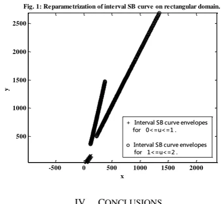
Simulation results in Figure (1), shows the reparametrization of the interval Said-Ball curve on rectangular domain in the range , -.
IV. CONCLUSIONS
In this paper a new representation forms of parametric interval Said-Ball curves is presented. This concept has been discussed to form a new curve , -( ) over rectangular domain such that its parameter varies in an arbitrary range , - where and are real, instead of ( )
, -( ) that’s defined by interval control points
*, -+ and its parameter varies in the range , -. The problem is to find a new interval Said-Ball curve , -( ), where , that’s defined by interval control points *, -+ such that the curve , -( ) based on them will go from . ( ) , -( )/ to
. ( ) , -( )/ i.e., and ( ( ) , -( ))
. ( ) , -( )/and will be identical in shape to , -( ) in that interval. Similarly, a new curve , -( ) over rectangular domain is obtained such that its parameter varies in the range , -, instead of ( )
, -( ) that’s defined by interval control points
*, ̃ ̃ -+ and its parameter varies in the range , -, in this case the problem is to find a new interval Said-Ball curve , -( ), where , that’s defined by interval control points {[ ̃ ̃ ]}
such that the curve , -( ) based on them will go from . ( ) , -( )/ to
. ( ) , -( )/ i.e., and ( ( ) , -( ))
-500 0 500 1000 1500 2000
500 1000 1500 2000 2500
x
y
Fig. 1: Reparametrization of interval SB curve on rectangular domain.
+ Interval SB curve envelopes for 0<=u<=1 .
. ( ) , -( )/and will be identical in shape to , -( ) in that interval. The four fixed Kharitonov's polynomials (four fixed SB curves) associated with the original interval Said-Ball curve are obtained. A new parameterization is applied to the four fixed Kharitonov's polynomials (four fixed SB curves). Finally, the required interval control points are obtained from the fixed control points of the four fixed SB curves. In CAD it is both convenient and practical to use the matrix form in representing parametric curves and surfaces. One of the reasons is that the matrix notation allows an easy conversion between different shape representations and provides a convenient implementation in either hardware or software with available matrix facilities. Using matrix representation, it has been shown how to determine the control points that covers an arbitrary interval , - of the original interval Said-Ball curve. Also, any change in the shape of the curve often causes the initial parametrization to be lost and hence reparametrization which preserves the shape of the curve is required, which can be done in terms of certain weight relations that are preserved by reparametrization.
REFERENCES
[1] P. Bezier, "Definition Numerique Des Courbes et ̂ I", Automatisme, Vol. 11, pp. 625–632, 1966.
[2] P. Bezier, "Definition Numerique Des Courbes et ̂ II", Automatisme, Vol. 12, pp. 17–21, 1967.
[3] P. Bezier, Numerical control, Mathematics and Applications, New York: Wiley, 1972.
[4] P. Bezier, The Mathematical Basis of the UNISURF CAD
System, Butterworth, London, 1986.
[5] H. B. Said, "A generalized Ball curve and its recursive algorithm", ACM. Transaction on Graphics, Vol. 8, No. 4, pp. 360–371, 1989.
[6] A. A. Ball, “CONSURF Part 1: Introduction to conic lofting tile”, Computer Aided Design, Vol. 6, No. 4, pp. 243–249, 1974.
[7] A. A. Ball, ”CONSURF Part 2: Description of the algorithms”,
Computer Aided Design, Vol. 7, No. 4, pp. 237–242, 1975. [8] A. A. Ball, “CONSURF Part 3: How the program is used”,
Computer Aided Design, Vol. 9, No. 1, pp. 9–12, 1977. [9] G. J. Wang, "Ball curve of high degree and its geometric
properties", Applied. Mathematics: A Journal of Chinese Universities Vol. 2, pp. 126-140, 1987.
[10] J. Delgado and J. M. Pena, “A linear complexity algorithm for the Bernstein basis”, Proceedings of the 2003 International Conference on Geometric Modeling and Graphics (GMAG’03), pp. 162–167, 2003.
[11] J. Delgado and J. M. Pena, "A shape preserving representation with an evaluation algorithm of linear complexity”, Computer Aided Geometric Design, pp. 1-10, 2003.
[12] T. W. Sederberg and R. T. Farouki, “Approximation by interval Bezier curves”, IEEE Comput. Graph. Appl., No, 2, Vol. 15, pp. 87-95, 1992.
[13] V. L. Kharitonov, "Asymptotic stability of an equilibrium position of a family of system of linear differential equations", Differential 'nye Urauneniya, vol. 14, pp. 2086-2088, 1978.
O. Ismail (M’97–SM’04) received the B. E. degree in electrical and
electronic engineering from the University of Aleppo, Syria in 1986. From 1987 to 1991, he was with the Faculty of Electrical and Electronic Engineering of that university. He has an M. Tech. (Master of Technology) and a Ph.D. both in modeling and simulation from the Indian Institute of Technology, Bombay, in 1993 and 1997, respectively. Dr. Ismail is a Senior Member of IEEE. Life Time Membership of International Journals of Engineering & Sciences (IJENS) andResearchers Promotion Group (RPG). His main fields of research include computer graphics, computer aided analysis and design (CAAD), computer simulation and modeling, digital
image processing, pattern recognition, robust control, modeling and identification of systems with structured and unstructured uncertainties. He has published more than 67 refereed journals and conferences papers on these subjects. In 1997 he joined the Department of Computer Engineering at the Faculty of Electrical and Electronic Engineering in University of Aleppo, Syria.
In 2004 he joined Department of Computer Science, Faculty of Computer Science and Engineering, Taibah University, K.S.A. as an associate professor for six years.