Power Consumption and Energy Estimation in Smartphones

(1)

International Journal of Advanced Engineering, Management and Science (IJAEMS) [Vol-2, Issue-10, Oct- 2016] Infogain Publication (Infogainpublication.com) ISSN : 2454-1311

www.ijaems.com Page | 1758

Power Consumption and Energy Estimation in

Smartphones

Ahmed Alsheikhy

1

, Reda Ammar

2

, Raafat Elfouly

3

,

Mosleh Alharthi

4

1_{Department of Electrical Engineering, Northern Border University, Arar, Saudi Arabia} 2

Department of Computer Science and Engineering, University of Connecticut, Storrs, USA

3_{Department of Computer Engineering, Cairo University, Cairo, Egypt} 4_{Department of Electrical Engineering, Taif University, Taif, Saudi Arabia}

Abstract— A developer needs to evaluate software

performance metrics such as power consumption at an early stage of design phase to make a device or a software efficient especially in real-time embedded systems. Constructing performance models and evaluation techniques of a given system requires a significant effort. This paper presents a framework to bridge between a Functional Modeling Approach such as FSM, UML etc. and an Analytical (Mathematical) Modeling Approach such as Hierarchical Performance Modeling (HPM) as a technique to find the expected average power consumption for different layers of abstractions. A Hierarchical Generic FSM “HGFSM” is developed to be used in order to estimate the expected average power. A case study is presented to illustrate the concepts of how the framework is used to estimate the average power and energy produced.

Keywords— Finite State Machine (FSM), Hierarchical Performance Model (HPM), Power consumption, Real-time embedded systems, Smartphones.

I. INTRODUCTION

In today’s world, using embedded systems is rising up extremely rapidly [1]. Many of those systems run on batteries and power consumption is considered to be an important criteria throughout the design process of an implementation [1,2,3,4]. Very often, a designer has to rely on a simulation tool to take a decision about which design is the best among others. Sometimes that tool can be particularly time consuming or insufficient. Due to heavy demands on embedded systems, it is essential to estimate performance metrics such as the delay and power consumption. The focus of performance analysis methods for real-time embedded systems is more on the analysis of timing aspects and power consumption [1,2]. In particular, a designer intends to determine which design produces less power while a system meets its real-time requirements [2,3]. A performance modeling scheme is required to evaluate the power consumption caused by communication and computation by distributed system architectures and existing software on different platforms

[1,3,4,5]; and also to identify where bottlenecks occur. Engineers rely on performance modeling to predict the expected power before moving to the final stage of implementation. However, in the absence of a performance evaluation scheme, they must design and implement a system to predict the performance defects or bottleneck. Waiting to spot the performance defects or bottleneck to occur until the final stage of implementation and integration between different components results in increased project costs, reduced productivity and delays in schedule [1,2,3,6]; applying performance modeling and evaluation from the first stage of design in any system exhibits better results than those using a “fix-it-later” approach [1,6]. Currently, three approaches exist that evaluate system performance and analysis which are: 1- Simulation Based Method, 2- Analytical Based Method and 3- Direct Measurement [1]. The Hierarchical Performance Model (HPM) combines and collaborates direct measurements with the analytical approach with the help of software performance engineering [2,3,4,5], queueing networks [6], hardware and software co-design to predict the average power consumption.

Our contribution in this paper is done by developing the hierarchical generic FSM, converting it to a Markovian model and also integrating it with its affiliated hierarchical performance model (HPM) in order to estimate system performance metrics such as power consumption and time delay. Only power consumption is considered in this paper. The developed framework was applied only on one device due to the availability and presented within this paper.

(2)

Infogain Publication (Infogainpublication.com) ISSN : 2454-1311

II. RELATEDWORK

Functional Modeling techniques and Analytical Modeling ones are used to estimate the system performance metrics such as power estimation at an early stage if possible. Queueing schemes have been used since the 1970s to model performance metrics of any software systems [6]. An FSM is used to evaluate system level performance [9,10,11]; however, that FSM was not applicable to any system since it was designed for a specific system. So designing a hierarchical generic FSM to be used in evaluating performance for any embedded system is developed in section 3. Many techniques were developed to estimate the power consumption at gate-level, circuit-level and register-transistor-level. However, those approaches are impractical to evaluate power consumption due to the lack of availability of circuit and gate levels information of a system under investigation. In [4], power analysis was done based on Y-chart scheme by Amit Nandi. He integrated power and performance analysis into the system level and claimed that the analysis became an integral part of the design process as it helped to find a proper architecture for a target application. Arafat, Ammar and Fergany in [8] applied the HPM method to evaluate the software power consumption based on measurements of the consumed power by each instruction. They claimed that their approach can be used to estimate power consumption of a software application based on physical measurements and computation modeling. In [13], rapid performance and power consumption evaluations were done at the system level only and that did not include the task level, module level and operations level. Kumar, Ben Attallah, Niar, Senn and Dekeyser in [14] presented a fast and accurate hybrid power estimation methodology for embedded systems at the system level only and did not provide any information about more levels. Many methods were developed to estimate the power consumption at the system level only as in [15].

Numerous parameters are required for each layer when using HPM to estimate the average power consumption in different levels; those parameters propagate from a bottom level to a higher one [1,2,3]. Nevertheless, accessing this information within a level or communication of information between these layers result in a complex manner [3]. The HPM is used to manage and distribute performance information between different layers of the framework. This paper considers the problem of mapping a functional modeling approach such as FSM to the analytical (mathematical) modeling approach such as (HPM) for performance analysis. A general overview of the developed framework using the functional modeling approach “HGFSM” which refers to Hierarchical Generic

Finite State Machine and the analytical modeling

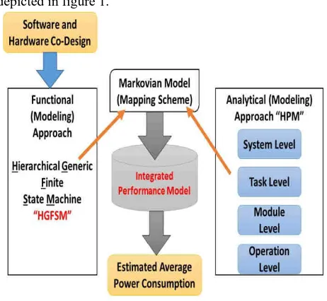
approach (HPM) to estimate the power consumption is depicted in figure 1.

Fig.1: developed framework

Hierarchical Generic FSM is designed and then converted into the Markovian Model “MM”. Each state in the Markovian model is decomposed into another sub-markovian states if possible. Furthermore, Hierarchical Performance Model “HPM” is applied to each state to derive the expected average power consumption equation(s) using bottom-up methodology which represent(s) the objective function(s).

III. HIERARCHICALGENERICFINITESTATE

MACHINEANDHIERARCHICAL

PERFORMANCEMODEL

A typical FSM model is composed of 5-tuples {∑ S, S0, δ,

F}; where: ∑ represents a set of input alphabets. S represents a set of states in the model. S0 represents an

initial state or a set of states which are sub-elements of S. δ

represents a state-transition function which maps between a current state to a next state and F contains a final state or a set of states which belongs to S [9,10]. A task in any embedded system can be classified as either completed or failed. A set of states exists among those two states to form the hierarchical generic FSM “HGFSM” model as shown in fig. 2 [1,2].

(3)

Each input alphabet is represented by a task or a set of tasks which are integrated to form a desired job. Movement from a current state Si to a next state Sj is

represented by a transition arrow and is done according to some existing circumstances or activities inside the system under investigation. For the hierarchical generic FSM, S contains all 7 states whereas S0 contains only one state

which is the Initial state. F contains one state which is named as completed state, referring to a successful completion, and is denoted by two circles in fig. 2. The states are: Initial state: each task is provided with an arrival time (ta) and a deadline time (td) which refer to one

of the constraints in the system. There is no transition

when the system is idle which means there is no incoming task. Checking state: it performs several tasks: • Checks if the task deadline can be met or not; if not, it forwards the task into the Failed state to restart its cycle. Otherwise, it moves to a next condition.

• Checks available resources for execution; if not, sends tasks to the Suspend state. Otherwise, performs the next operation.

• Checks if the queue in the Execution state, which is also called the Processing state as shown in fig .2, is full or not; if not, then it forwards the task into the Execution “Processing” state. Otherwise, it forwards it into the waiting state.

The state itself is decomposed into another sub-FSM which contains 3 states: Receiving and checking state,

Decision State and Recording state. More information

can be found in [1]. The Execution “Processing as in fig. 2” state: represents the place where the task is executed. If the execution is done successfully, it sends the task to the Completed state. Otherwise, it sends it to the Failed state. The execution is completed successfully if the execution time (te) <= deadline time (td). The state is decomposed

into another two sub-FSMs to form hierarchical model as shown in fig. 2. In the Waiting state, the task waits its turn to be executed once the queue of the Execution “Processing” state is not full or the Processing Unit “P.U.” becomes available when the deadline time can be met; otherwise, the task is sent to the Failed state to restart its cycle. The Suspend state, contains tasks for which their computing resources are not yet available and there is a high chance to be executed once their resources become available while the deadline time can be met. There are 16 states in the developed HGFSM which form the complete model. The HGFSM in fig. 2 can be remodeled by including the Suspend state inside the Checking state, more information about it can be found in [1].

The hierarchical generic FSM is mapped to a Markov model “MM” which represents a state diagram (a component of HPM) [1,2]. The Markovian model has

3-tuples {S, A, P}, where S represents a set of states existed in the HGFSM model. A denotes a vector of initial probabilities values for all states in the model while P contains a matrix that represents transition probabilities among states according to some circumstances existed in the developed model. The mapping is done as follows: 1. Every state in the HGFSM is mapped to a state in the MM. 2. Each edge in the HGFSM is converted to a transition arrow qij which represents the flow direction from the

current state (Si) to the next state (Sj). 3. Each transition

arrow is associated with a parameter kij which represents a

number of tasks that go from state Si to state Sj. That

parameter is used to calculate the probability value Pij

which denotes the possibility of moving from the current state (Si) to the next state (Sj) and it is calculated using the

following equation, where Ni represents a number of total

tasks in state Si

Pij = Kij / Ni (1)

4. Each FSM graph and state is associated with its Computation Structure Model “CSM” to show data flow in the system under consideration. CSM helps in constructing performance metrics equations. 5. If applicable, a state is decomposed into another sub-FSM and additional Markovian model is constructed to create another level in the hierarchy. A figure for the Markovian model is not shown in this paper due to the space limitation. However, the interested readers can found more information about it in [1].

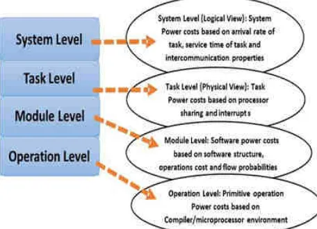
Performance modeling evaluation is considered to be the abstraction of the functional and performance characteristics of the system under consideration which are combined to determine if it meets the performance requirements based on a user demands and system architectures [6,16]. The Hierarchical Performance Model (HPM) layers are illustrated in figure 3. There are 4 layers in fig. 3 which are used to derive the average power consumption and the average energy produced in the system(s) under investigation.

(4)

Infogain Publication (Infogainpublication.com

IV. CASESTUDY:ANDROID

Android software architecture is designed and built as a stack structure as depicted in fig. 4(a) [18].

Fig. 4(a): Android software architecture

All components of the 4 layers integrate with each other to form what is known today as ANDROID

contains some blocks that integrate together to do a set of specific jobs. The 4 major layers “levels” in Android from bottom to up are: A. LINUX KERNEL, B. LIBRARIES AND ANDROID RUNTIME, C. APPLICATION FRAMEWORK and D. APPLICATIONS. More information can be found in [18,19,20,21].

Any application in Android is built based on 4 different components which are: 1- Activity, 2- Content provider, 3 Service and 4- Broadcast receiver [19,20,21]. In Android, a task can be defined as an activity or a set of activities. A typical lifecycle for any activity in Android has 7 states which are: OnCreate, OnStart, OnResume, OnPause, OnRestart, OnStop and OnDestroy. Interested readers are referred to [18,19] for more details about Android. Table 1 illustrates the mapping between the HGFSM and the Android activity lifecycle.

Infogainpublication.com)

ANDROID

Android software architecture is designed and built as a 4(a) [18].

4(a): Android software architecture

All components of the 4 layers integrate with each other to

ANDROID. Each layer

contains some blocks that integrate together to do a set of specific jobs. The 4 major layers “levels” in Android from RNEL, B. LIBRARIES AND ANDROID RUNTIME, C. APPLICATION FRAMEWORK and D. APPLICATIONS. More information can be found in [18,19,20,21].

Any application in Android is built based on 4 different Content provider, 3- Broadcast receiver [19,20,21]. In Android, a task can be defined as an activity or a set of activities. A typical lifecycle for any activity in Android has 7 states which are: OnCreate, OnStart, OnResume, OnPause, Interested readers are referred to [18,19] for more details about Android. Table 1 illustrates the mapping between the HGFSM and the

Table.1: Mapping HGFSM with the Android activity lifecycle

Fig. 4(b) shows a typical overview of how a task starts and runs on an Android device.

Fig. 4(b): Task execution in Android

In fig. 4(b), solid lines indicate the control flow between the states whereas the dashed lines indicate a message that is sent among states. Once the software processes, which are displayed as the states, and the interface messages between all states are known, our next step is to determine the performance parameters associated with the graph. These parameters are: Tasks arrival rates

tasks exist in each state before processing them N number of tasks move from the current state (S new state (Sj) Kij, flow probabilities P

multipliers βij, which are assumed to be unity, and lastly the computation and

(service) times E(s). To utilize the performance

parameters, at the early stage, we identify the input(s), output(s) and divide any Android system into different components if possible as shown in figure 4(c). There are

ISSN : 2454-1311

Table.1: Mapping HGFSM with the Android activity lifecycle

4(b) shows a typical overview of how a task starts and

4(b): Task execution in Android

In fig. 4(b), solid lines indicate the control flow between the states whereas the dashed lines indicate a message that states. Once the software processes, which are displayed as the states, and the interface messages between all states are known, our next step is to determine the performance parameters associated with the graph.

Tasks arrival rates λ, number of tasks exist in each state before processing them Ni, number of tasks move from the current state (Si) to the , flow probabilities Pij, message , which are assumed to be unity, and lastly the computation and communication cost

(5)

one input, one output, six components (one action, one

sequence and four branches).

Fig.4(c): System Components

To determine the probabilities values, we need to know how many tasks (Ni) exist first in each state and then how

many tasks (kij) out of Ni are sent from state Si to state Sj;

all these numbers should be known in advance either by obtaining them from actual tests (experiments/simulation) or given by the designers. Several experiments were performed in order to obtain the values for different performance parameters to estimate the expected average power consumption and/or energy produced. Table 2 shows the number of tasks exist in each state while the system under investigation is running. Note that the subscript indicates the state (ID). The system within this paper will be represented by a smartphone, more specific, Galaxy Note 3 is the system to be used and tested.

Table.2: Number of tasks in each state

The probability value Pij is computed using equation (1);

the next step is to specify the details of the methods used to derive the power consumption equation(s). The software structure indicates the order in which the operations are executed in order to complete a desired task or computation. The software structure can be seen as the

Computation Structure Method (CSM) which consists

of Data Flow Graph DFG and Control Flow Graph CFG. The DFG and CFG for the Android application are not shown due to the space limitation. The interested readers are referred to [1] for more information and DFG and CFG. To derive a cost equation, we multiply each state cost with its associated flow parameter; then sum all results. After substituting all dependent flows with independent ones, the independent flows are that which complete loop whereas the dependent flows are the

remaining ones. The expected average power consumption is computed as follows:

PCaverage=(1*Cinitial)+((1+e4)*(Ccheck+Ctest))+((e11+1)*Cdeci sion)+((e9+e8)*(Cwait+Ctest))+((e11+1)*(Cexe+Ctest) (2)

PC stands for Power Consumption. To compute the energy produced from the system, just multiply the result from eq. (2) with a time (t) spent to perform the desired jobs. In equation (2), each parameter is associated with its flow variable(s) which is/are denoted by e. Each flow variable represents a value of moving through a path from a start node to an end node in the CFG. Each flow takes a value between {0,1,….,∞} and mainly depends on a type of distribution [1,2]. The flows also represent the data dependent aspects of the computation time [1]. They are discrete random variables and are modeled using probability distribution and statistics methods. Several probability distributions exist which are summarized as follows: Bernoulli, Binomial, Geometric, Modified

Geometric and Poisson [1,2]. Given the probability

distribution type of e, several characteristics such as Expected value E(e), second moment E(e2), Variance Var(e) and the coefficient of variation C2 are easily obtained. More information about estimating the values of computations and communication aspects can be found in [1,3]. The value of Cinitial is determined from its CFG as

shown in fig. 5(a). From fig. 5(a), three operations take place in every Android device which are: Assigning thread to perform a desired action, Variables initialization and finally creating the Graphical User Interface to interact with a user.

Fig. 5(a): CFG for the Initial state

From fig. 5(a), the equation for estimating the average power consumption is computed as follows:

Cinitial = Ccreate UI + CInitializations + Cassigning thread (3)

For the Executing “Processing” state, its cost is obtained from its CFG which is now shown due to the space limitation; so

Cexecution = [(e1+e4)*(Chandling state+Ctest)]+[e4*Caborted]

+[(1+e4)*Ctest] (4)

Initial Check Wait Execution Failed

(6)

Infogain Publication (Infogainpublication.com) ISSN : 2454-1311

Substitute the value of Chandling state which is obtained from

its CFG as depicted in fig. 5(b).

Chandling = [(1 + e3 + e6) * (Cready + Ctest)] + (e3 * Cidle) +

[(e6+1)*Ctest]+(1*(Crun)) (5)

Note that the cost value obtained for each state represents the expected power consumption which is used for the computation in a Node View in the system level [1].

Fig. 5(b): CFG of the Handling state

Next step is to find a number of visits V to each state which is computed using the following equation

[V] = (I – P)-1 (6) Where [V] is a matrix whose elements indicate number of visits to each state; the number of its entries is equal to the number of states exist in the system. I is the identity matrix and P is the matrix of transition probabilities between all states. So the average cost becomes as follows:

PCaverage = ∑(Vi*Ci) (7)

Where i = 1,……..,6 which is the number of states in the framework; Ci indicates the value of cost associated with

each state.

Only one hardware architecture was used, due to the availability reason, to profile different applications. A profiler tool used to find the actual power consumption in the smartphones is available only on limited devices. JAVA Eclipse is also used to estimate the values of several performance parameters by performing multiple experiments. The architecture refer to a Smartphone, run with Android as O.S., which is: Galaxy Note 3 as mentioned earlier. The applications used within this profiling part range from a simple one like a Basic

Calculator to more complex one, which consumes more

power from the P.U. such as Video Recording. Four

different applications were used including: 1. Video Recording with Preview, 2. Calculator, 3. Audio Recording, and 4. Picture Taking. The profiling was done in three parts according to the developed HGFSM which are:

Initial part (part one in the developed HGFSM): represents the first stage toward finding the average power consumption for a task. This stage contains “Initial state” in the HGFSM and “OnCreate” in the Android activity lifecycle. Check part (part one in the developed HGFSM): represents the second stage and contains two states which are (the Checking State and the Waiting state in the HGFSM) and (OnStart) in the Android activity lifecycle as shown in table 1. Run part (part two and three in the HGFSM): represents the last stage and contains the following states: Execution, Completed and Failed as shown in table 1.

The aim of this profiling is to determine the expected average power consumption and to identify which part in the smartphone produces more energy. All applications were tested several times (about 50 times) and then the average power is determined. In the architecture, all four applications were installed and then the profiling started by launching them one by one. For flows in equations (2) to (5), they occur in a single run of “if statement” and we assume equally likely for a branch to be taken so p = q = 0.5 since p + q = 1 as stated earlier.

Finding the number of visits in each state is determined using Matlab and then substituting in equation (2) will give the expected average power cost as follows;

E(PC)=(1*Cinitial)+(E(1+e4)*(Ccheck+Ctest))+(E(e11+1)*Cde cision)+(E(e9+e8)*(Cwait+Ctest))+(E(e11+1)*(Cexe+Ctest) (8)

E refers to Expected average value, so the average energy produced is calculated using the following equation: E(energy) = E(Power) * t (9) Where t represents the period of time taken to run the applications and it is fixed to be 45s = 45000ms. Tables 3 shows the actual values and expected ones for power consumption for all 4 applications in Note 3.

Table.3: actual and expected power consumption in Note 3

Application Name

Expected power (mw)

Actual Power (mw)

Error

Video 2.215 1.997 10.92% Calculator 1.743 1.856 6.09%

Audio 2.189 1.972 11% Taking

(7)

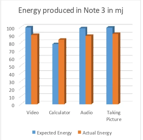
The difference between the expected and actual average power consumption lays within a small error “±11” as shown in table 3. Table 4 illustrates the actual and the expected average energy produced in Note 3 in milli joule “mj”; all values are scaled by 103.

Table.4: expected and actual energy produced in Note 3 Application

Name

Expected Energy (mj)

Actual

Energy(mj) Error Video 99.675 89.865 10.92% Calculator 78.435 83.52 6.09%

Audio 98.505 88.74 11% Taking

Picture 99.27 91.485 8.51%

Fig. 6 shows the actual and expected energy produced in Note 3 by all four applications with scale by 103.

Fig. 6: expected and actual energy in Note 3

Samsung tried to minimize the energy produced in its devices and Note 3 yields less than expected even though that several applications were already installed and run on it. During the experiments, several applications ran on Note 3 and caused he energy to be higher than the expected. Also the initial state, which includes several activities (assigning thread, variables initializations and creating the GUI), consumes more power than the remaining states. In general, the Note 3 device is optimized in terms of the power consumption and the execution time as proofed by the experiments. Table 5 illustrates the average values for several primitives operations in Samsung Galaxy Note 3 after performing different experiments. All values are in milli watt “mw” and were obtained after repeating the experiments more than 45 times.

Table.5: List of primitive operations and their average power consumption values

List of primitive

operations Average value Function call 0.0437

Addition 0.119 Subtraction 0.147 Multiplication 0.492 Division 0.687

Fig. 7 illustrates the average power consumption (actual and expected) in Galaxy Note 3 using two benchmark applications. The two benchmark applications are Mobibench and Norvigtorious, both of them can be found and downloaded from Play Store or from Github. They were tested and ran several times to estimate the average values.

Fig.7: Average power consumption in two benchmarks

In each benchmark application, the first bar refers to the actual average power consumption while the second bar represents the estimated average values.

V. CONCLUSION

This paper presented the developed framework to estimate the expected average power consumption and energy in smartphones which incorporated different levels of abstraction. Two examples were given to demonstrate how the power and energy are estimated using the software structure and the architecture to represent the corresponding levels of the model. The framework can be applied on any smartphone to estimate the expected average values for the power consumption and the energy produced. The future work is to determine the average power dissipation and energy consumed with a device runs on multiple threads “up to three threads” and find the effect of rendering GPU(s) to take control on creating graphical task(s) such as drawing the UI window which is found to be the dominant factor. It takes about 75% of the average power cost in the Initial state.

0 10 20 30 40 50 60 70 80 90 100

Video Calculator Audio Taking

Picture

Energy produced in Note 3 in mj

(8)

Infogain Publication (Infogainpublication.com) ISSN : 2454-1311 REFERENCES

[1] A. Alsheikhy, “High Performance Embedded System”, Doctoral Dissertation, University of Connecticut, 2016.

[2] A. Alsheikhy, S. Han and R. Ammar, "Hierarchical Performance Modeling of Embedded Systems“, Computers and Communication (ISCC), 2015 20th IEEE Symposium on Computers and Communications, pp. 936-942, July 2015.

[3] A. Alsheikhy, S. Han and R. Ammar, "Delay and Power Consumption Estimation in Embedded Systems Using Hierarchical Performance Modeling”, 15th IEEE International Symposium on Signal Processing and Information Technology (ISSPIT), pp. 34-39, December 2015, Abu Dhabi, UAE. [4] A. Nandi, “System-Level Power/Performance

Analysis for Embedded Systems Design”, Master Thesis, Carnegie Mellon, 2002.

[5] L. Chin, .S. Wei and G. Yu, ”Performance Evaluation of Embedded System Based on Behavior Expressions”, 2nd International Conference on Mechanical and Electronics Engineering (ICMEE), Vol. 1, pp. 253-256, 2010.

[6] D. Smarkusky, R. Ammar, I. Antonios and H. Sholl, “Hierarchical Performance Modeling for Distributed System Architectures,” Computer and Communications, 2000. Proceedings. ISCC 2000. Fifth IEEE Symposium, pp. 659–664, July 2000. [7] R. Ammar, “Software Performance Analysis,”

lecture notes, University of Connecticut, 1991. [8] H. Arafat, R. Ammar and T. Fergany, “Evaluating

Software’s Power Consumption”, Paper Version, University of Connecticut.

[9] B. Lee and E. A. Lee, “Interaction of Finite State Machines and Concurrency Models”, Proceeding of Thirty Second Annual Asilomar Conference on Signals, Systems and Computers, Pacific Grove, California, November 1998.

[10]A. Stan, N. Botezatu, L. Panduru and R. G. Lupu, “A Finite State Machine Model Used in Embedded Systems Software Development,”, pp. 51-63, 2009. [11] B. Lee and E. A. Lee, “Hierarchical Concurrent

Finite State Machines in Ptolemy,”, Proceeding of International Conference on Application of Concurrency to System Design, pp. 30-40, Fukushima, Japan, March, 1998.

[12] M. Sarrafzadeh, F. Dabiri, R. Jafari, T. Massey and A. Nahapetian, “Low Power Light-Weight Embedded Systems”, Proceedings of the International Symposium on Low Power Electronics and Design (ISLPED), pp. 207-212, Oct. 2006. [13] S. Niar and N. Inglart, “Rapid Performance and

Power Consumption Estimation Methods for

Embedded System Design”, Proceedings of the 7th IEEE International Workshop on Rapid System Prototyping (RSP), 2006.

[14] S. Kumar, R. B. Attallah, S. Niar, E. Senn and J. L. Dekeyser, “Fast and Accurate Hybrid Power Estimation Methodology for Embedded Systems”, Conference on Design and Architectures for Signal and Image Processing (DASIP), IEEE, pp. 1-7, 2011. [15] S. Kumar, O. Palomar, O. Unsal, A. Cristal, R. B.

Attallah and S. Niar, “PETS: Power and Energy Estimation Tool at System-Level”, 15th International Symposium on Quality Electronic Design (ISQED), pp. 535-542, 2014.

[16] J. Viskari, R. Jokinen and K. Hakkarainen, “A Generic FSM Interpreter for Embedded Systems,”, proceedings of IEEE EURWRTS, pp. 284-289, 96. [17] L. Carmichael, A. Warner, FNAL and Batavia, “A

Generic Finite State Machine Framework for the ACNET Control System,”, proceedings of ICALEPCS, pp. 28-30, Kobe, Japan, 2009.

[18] Z. Wang and A. Stavrou, “Google Android Platform: Introduction to The Android API, HAL and SDK,”, lecture notes, George Mason University.

[19] V. Matos, “Android Multi-Threading,” Notes on Android, Chapter 13, Cleveland State University. [20] X. Ma, “Android OS,”, lecture notes, CSE 120, Fall

2010.

[21] S. Brahler, “Analysis of The Android Architecture,”, master thesis, Karlsruher Institute for Technology, October 2010.