314
Comparative Analysis Of Methods Of Baseflow
Separation Of Otamiri Catchment
Nwakpuda Nat. I.
ABSTRACT: The various approaches of separating baseflow from other streamflow components are hinged on their respective strengths and drawbacks with respect to the watershed considered. Little wonder therefore, that this research work has ventured on some methods amongst multitude of emerged methods, to establish the best method(s) of baseflow separation and henceforth address the strength and drawback dichotomy associated with the different baseflow separation methods. The examined methods of baseflow separation used in this work are conveniently categorized into five basic approaches of fixed interval, sliding interval, local minimum, Baseflow Index and frequency analysis. Data for the analyses obtained from Otamiri River at Nekede were utilized for this study and daily recorded streamflow discharge data obtained from the historical records held at the libraries of the Anambra Imo River Basin Development Authority, Owerri and the Nigerian National Meteorological Services. The results of the predictability of the stream flow from the estimated baseflow for all the methods used conformed as evident in the regression analysis and the results showed that the value of the coefficient of simple determination (r2) was highest in the fixed interval method and least in the frequency analysis method which implies that the fixed interval method was the best method of separating the base flows for Otamiri stream.
Keywords: Baseflow separation, Otamiri streamflow, fived interval, Sliding Interval, Local Minimum, Baseflow index, Frequency analysis.
———————————————————
1
INTRODUCTION
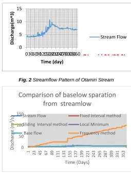
Runoff hydrograph usually consists of a fairly regular lower portion those changes slowly throughout the year and a rapidly fluctuating component that represents the immediate response to rainfall. The lower, slowly changing portion of runoff is termed base flow. The rapidly fluctuating component is called direct runoff. This distinction is made because the unit hydrograph is essentially a tool for determining the direct runoff response to rainfall. hydrologists and hydro-geologists, generally depending on either the number of components the total flow can be separated into, or the subjective nature of the method of separation. Baseflow separation is the process whereby stream flow hydrograph is separated into its relevant components. The number of water sources or components that contribute to the stream flow can be identified depending on the conceptual model of flow. Some models consider two components of flow (i) Quick flow – the direct response to a rainfall event including overland flow (runoff), lateral movement in the soil profile (interflow) and direct rainfall onto the stream surface (direct precipitation, and (ii), Baseflow – the longer-term discharge derived from natural storages, whereas other models consider more than two components of flow. Analyzing the baseflow component of the streamflow hydrograph has had long history of development since the early theoretical and empirical work of Boussinesq (1904), Maillet (1905) and Horton (1933).
Several useful reviews have been postulated including Hall (1968), Nathan and McMahon (1990), Tallaksen (1995) and Smakhtin (2011) to map this development. The conceptual basis for such analysis can only really apply in small catchments where differential travel times, due to distance from the catchment outlet, play minor role. In larger catchments such as the Imo River Basin the situation is far more complex as baseflow can be affected by a multitude of processes, some dominated by topography, others by subsurface (soils and geology) characteristics and others by spatial variations in rainfall inputs. Further complexities are intensified when runoff processes are considered in more detail. A number of field studies have demonstrated that subsurface runoff processes in some catchments can operate at quite rapid rates (Ward, 2004; Putty and Prasad, 2010), while surface runoff on hill slopes may be re-infiltrated further downslope. It is apparent that, apart from a very few experimental catchments which are comprehensively instrumented, it is extremely difficult to determine what component of the total flow hydrograph can be considered as baseflow. Chemical and isotope tracing studies (Marc et al., 2001), as well as simulation modelling (Haberlandt et al., 2001) offer alternative methods for hydrograph separations, however, they all require extensive time and manpower resources. The study is designed to address the issue of baseflow separation, analyzing and comparing various methods aiming at recommending the most appropriate derived/adopted method for the Anambra Imo River Basin catchment [specifically, the Oramiriukwa River and Otamiri River] of Owerri, Imo State, Nigeria. This also would be applicable / useable in other areas/regions of the country. This is achievable by categorizing the various existing methods of baseflow separation, comparing them and identifying the most appropriate method for adoption for use in baseflow separation to aid design and management purposes. The key objectives of this study are as follows: I. Collection of rainfall data [runoff] from the catchment
area isolated -- Owerri, Imo State. The driest period is picked as the measured baseflow figure used as a standard for comparison,
II. Separation of the baseflow from the runoff using the known methods for comparison,
_______________________
Nwakpuda Nathaniel I. is currently pursuing Phd. degree program in water resource and Environmental Engineering in the Dept. of Civil Engineering, University of Nigeria,Nsukka, Nigeria, PH-08033401201. E-mail: [email protected]
III. Comparison of predicted baseflow from different methods with the observed data,
IV. Examining the relationship between the methods of analysis with the streamflow data,
V. Derivation of a modified method of baseflow estimation and its verification using observed data.
Graphical / Filtering Separation Methods
Graphical methods for hydrograph separation are useful for separating baseflow from individual storm events as against continual records of data. The technique does not consider physical parameters within catchments and so is arbitrary in nature, and. it is difficult to understand what the baseflow component actually represents. For instance the Gray’s (1973) method involves drawing a line backwards on the recession limb from the point at which direct runoff ends (point B See Fig.1) until it reaches under the peak of the hydrograph, and is then connected to the event marking the beginning of surface water runoff (point A). The Subramanya’s (1994) method is applied in a similar fashion except that the line is drawn backwards from the recession limb until it reaches the point of inflexion on the hydrograph. Graphical techniques that use analytical algorithms include one proposed by the United States Department of Agriculture – Agricultural Research Service (USDA-ARS, 1973) and Nazeer (1989). The method uses a mass balance approach and assumes a two component model. Three equations are used to separate baseflow into periods of recharge of soil moisture, recharge of groundwater and recession. In the first step of the technique by Nazeer (1989), any baseflow separation technique can be used to draw an approximation of the baseflow curve. In the second step, the shape factor of the baseflow curve is calculated (using an algorithm which is related to the time to peak streamflow). The shape of the approximated baseflow curve is procedurally altered until the shape factor correlates with the shape factor of the hydrograph curve.
Fig.1 Typical Example of Graphical baseflow separations.
Source: Gray (1973)
Graphical methods are commonly used to plot the baseflow component of a flood hydrograph event, including the point where the baseflow intersects the falling limb. Stream flow subsequent to this point is assumed to be entirely baseflow, until the start of the hydrographic response to the next significant rainfall event. These graphical approaches to partitioning baseflow vary in complexity and include: 1. An empirical relationship for estimating the point along
the falling limb where quickflow has ceased and all of
D = 0.827A0.2 (
Where D is the number of days between the storm crest and the end of quickflow, and A is the area of the catchment in square kilometers (Linsley et al. 1975). The value of the exponential constant (0.2) can vary depending on catchment characteristics such as slope, vegetation and geology.
i. The constant discharge method assumes that baseflow is constant during the storm hydrograph (Linsley et al. 1958). The minimum streamflow immediately prior to the rising limb is used as the constant value.
ii. The constant slope method connects the start of the rising limb with the inflection point on the receding limb. This assumes an instant response in baseflow to the rainfall event.
iii. The concave method attempts to represent the assumed initial decrease in baseflow during the climbing limb by projecting the declining hydrographic trend evident prior to the rainfall event to directly under the crest of the flood hydrograph (Linsley et al. 1958). This minimum is then connected to the inflection point on the receeding limb of storm hydrograph to model the delayed increase in baseflow.
iv. Using the trends of the falling limbs before and after the storm hydrograph to set the bounding limits for the baseflow component (Frohlich et al. 1994).
v. Use the Boussinesq equation as the basis for defining the point along the falling limb where all of the streamflow is baseflow (Szilagyi and Parlange 1998).
2.0
METHODOLOGY
2.1 Study Area
316 y = 0.960x + 0.061
r² = 0.952 r = 0.976
0.00 2.00 4.00 6.00 8.00 10.00 12.00
0.00 5.00 10.00 15.00
Esti
m
ate
d
D
isch
ar
ge
b
y
Fi
xed
In
te
rv
al
M
e
th
o
d
(m
3/s)
Stream flow (m3/s) winds known locally as the Harmattan, which usually
prevails December through March.
2.2 Fixed Interval Method
The fixed-interval method assigns the lowest discharge in each interval (2N*) to all days in that interval starting with the first day of the period of record. The method can be visualized as moving a bar 2N* days wide upward until the bar first intersects the hydrograph. The discharge at that point is assigned to all days in the interval. The bar is then moved 2N* days horizontally, and the process is repeated. The assigned values are then connected to define the base-flow hydrograph. The second technique for baseflow separation, the sliding-interval method, finds the lowest discharge in one half the interval minus 1 day [0.5(2N*-1) days] before and after the day being considered and assigns it to that day. The method can be visualized as moving a bar 2N* wide upward until it intersects the hydrograph. The discharge at that point is assigned to the median day in the interval. The bar then slides over to the next day, and the process is repeated. The assigned daily values are then connected to define the base-flow hydrograph. The Third method for this separation , the local-minimum method, checks each day to determine if it is the lowest discharge in one half the interval minus 1 day [0.5(2N*-1) days] before and after the day being considered. If it is, then it is a local minimum and is connected by straight lines to adjacent local minimums. The base-flow values for each day between local minimums are estimated by linear interpolations. The method can be visualized as connecting the lowest points on the hydrograph with straight lines. The fourth approach for this separation, the Base Flow Index (BFI), the index is calculated as the ratio of the flow under the separated hydrograph to the flow under the total hydrograph. The program calculates the minima of five-day non-overlapping consecutive periods and subsequently searches for turning points in this sequence of minima. The turning points are then connected to obtain the base flow hydrograph, which is constrained to equal the observed hydrograph ordinate on any day when the separated hydrograph exceeds the observed. The frequency duration analysis, the fifth approach for baseflow separation for this work, is a statistical assessment that uses the following relationship for flow data of fixed time period (daily, monthly or annual):
𝑃 = 100 (* +) (1)
Where: 𝑃 = the probability of a given flow that will be equaled or exceeded;
M = the ranked number when daily or monthly flows are arranged in descending order and
N = the total number of observations
3.
RESULT
PRESENTATIONS
AND
DISCUSSIONS
3.1 Result Presentations
The baseflow separation analysis results obtained from the daily recorded streamflow discharge data obtained from the historical records held at the libraries of the Anambra Imo River Basin Development Authority Owerri and the Nigerian National Meteorological Services; using the five methods as outlined above are presented below:
Fig. 2 Streamflow Pattern of Otamiri Stream
Fig. 3 Graphical display of Baseflow Separation from streamflow for all the methods employed.
Fig. 4 Predictability of the stream flow from the Base flow Discharge Using the Fixed Interval Method 0
5 10 15
0306090120150180210240270300330360
D
isch
ar
ge
(m
^3)
Time (day)
Stream Flow
Otamiri 81/82 Streamflow
0 50 100 150
1 23 45 67 89
111 133 155 177 199 221 243 265 287 309 331 353
Dis
ch
ar
ge
(m
3/s
)
Time (Days)
Comparison of baselow sparation
from streamlow
Stream Flow Fixed Interval method
Sliding Interval method Local Minimum
Fig. 5 Predictability of the stream flow from the Base flow Discharge Using the Sliding Interval Method
Fig. 6 Predictability of the Stream flow from the Baseflow Discharge Using the Local Minimum Method
Fig. 7 Predictability of the Stream flow from the Base flow Discharge Using the Base Flow Index Method
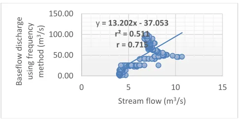
Fig. 8 Predictability of the Stream flow from the Base flow Discharge using the frequency Analysis Method
3.2DISCUSSIONS
The following points as captured in the regression analysis of all the methods of base flow separation as well as in the graphical comparison of the baseflow separation ability of all the employed techniques are sacrosanct, and the following discussions are evident. As seen from the estimated and presented results, the Fixed Interval Method of baseflow separation (Figure 4) has the highest value of the coefficient of simple determination (0.952), followed progressively by the BFI (figure 7) (0.943), Sliding Interval Method(Figure 5) (0.827), Local Minimum (figure 6) (0.811) and frequency analysis method (8) (0.340), it implies that the Fixed Internal Method is the best method of separating the base flow discharge., as it has the highest percentage accuracy (95.2%) more than any other base flow separation method. Moreover, the fixed Internal Method has the strongest positive relationship (the baseflow values will increase 97.6% linearly as the stream flow values increases) between the value of the base flow discharge separated and the streamflow (defined by its highest value of correlation coefficient of 0.976), compared to the values recorded for other methods. Therefore, the fixed interval method of base flow separation is the most accurate in separating the base flows as high as 95.2% efficient. This shows that the fixed internal method was the best method of separating the base flow for the Otamiri watershed.
4.
C
ONCLUSIONIndeed ,baseflow separation techniques will ever remain dogged as they have in no little measure offer a remedy to the critical challenge of understanding the dynamics of water management issues . Analyzing and separating the baseflow component of the stream hydrograph has had a long history of development since the early theoretical and empirical work of Boussinesq (1904), Maillet (1905) and Horton (1933). Several useful reviews have been written including Hall (1968), Nathan and McMahon (1990), Tallaksen (1995) and Smakhtin (2001) to map this development. Methods of achieving this will always penetrate so as to answer in a more sound way, limitations of various base flow separation techniques. Obviously, joy behooves and fresh hopes established as the fixed interval method, has emerged the most reliable of all for both watersheds. Conclusively, This Analysis has ascertained the best method of base flow separation from the stream flow from Otamiri stream and other streams of similar hydrological characteristics.
ACKNOWLEDGEMENT
In appreciation for the completion of this work, our profound thanks goes to God Almighty who has not relented in showing us mercy, love, care and grace in abundance throughout the period of this work. Our unreserved gratitude goes the editor and to all members of the publication and review team of the International Journal of scientific and Technological research (IJSTR); for their kind, timely, dedicated and meticulous critics which saw to the realization of this paper review and Publication. Alongside these pioneers, worthy of great appreciation here, is our friend, Engr. Patrick O. Aliboh whose contributions cannot be quantified. Engr. Emeka Udokporo, thank you as well. Last of these, would be our young student and friend with a y = 0.944x + 0.176
r² = 0.943 r = 0.971
0.00 2.00 4.00 6.00 8.00 10.00 12.00
0.00 5.00 10.00 15.00
Esti m ate d D isch ar ge b y B ase fl o w in d e x M e th o d (m 3/s)
Stream flow (m3/s)
y = 13.202x - 37.053 r² = 0.511
r = 0.715
0.00 50.00 100.00 150.00
0 5 10 15
Ba se flo w d is ch arg e u si n g fre q u en cy me th o d ( m 3/s )
Stream flow (m3/s)
y = 0.970x - 0.074 r² = 0.827
r = 0.909
0.00 2.00 4.00 6.00 8.00 10.00 12.00
0.00 5.00 10.00 15.00
Esti m ate d D isch ar ge b y Sl id in g In te rv al M e th o d (m 3/s)
Stream flow (m3/s)
y = 0.885x + 0.229 R² = 0.811
r = 0.901
0.00 5.00 10.00 15.00
0.00 5.00 10.00 15.00
Esti m ate d D isch ar ge b y Lo cal m in im u m M e th o d (m 3/s)
318 committed efforts in this work remain exceptional; thank you
! All the other persons who overtly or covertly contributed in making this work a success, a huge thank you!!!
R
EFERENCES[1]. Boussinesq J (1877) Essai sur la theories des eauxcourantes. Memoires presentes par divers savants a l’Academic des Sciences de l’Institut National de France, Tome XXIII, No 1.
[2]. Boussinesq J (1904) Recherchestheoretique sur l’ecoulement des nappes d’eauinfiltreesdans le sloet sur le debit des sources. J. Math. Pure Appl. 10 (5thSeries), 5-78.
[3]. Grayson RB, Argent RM, Nathan RJ, McMahon TA, Mein, RG (1996) Hydrological recipes: estimation techniques in Australian hydrology. CRC for Catchment Hydrology
[4]. Linsley, R. K., Kohler, M. A., and Paulhus, J. L. H. (1975) Hydrology for engineers, McGraw-Hill.
[5]. Linsley RK, Kohler MA, Paulhus JLH, Wallace JS (1958) Hydrology for engineers. McGraw Hill, New York.
[6]. Frohlich K, Frohlich W and Wittenberg H (1994) Determination of groundwater recharge by baseflow separation: regional analysis in northeast China. FRIEND: Flow Regimes from International Experimental and Network Data, Proceedings of Braunschweig Conference, October 1993. IAHS Publ. No 221
[7]. Maillet E (1905) Essaisd ’Hydraulique Souterraineet Fluviale. Hermann Paris, 218pp.
[8]. McDonnell, J. J. and Tanaka, T. (Eds.) (2001) Hydrology and biogeochemistry of forested catchments, Special issue of Hydrological Processes, 15(9).
[9]. Nathan RJ, McMahon TA (1990) Evaluation of automated techniques for base flow and recession analyses. Water Resources Research 26(7), 1465-1473.
[10]. SMAKHTIN VU (2001) Estimating continuous monthly baseflow time series and their possible applications in the context of the ecological reserve. Water SA
[11]. Smakhtin VU (2001) Low flow hydrology: a review. J Hydrology 240, 147-186.
[12]. Szilagyi J, Parlange MB (1998) Baseflow separation based on analytical solutions of the Boussinesq equation. Journal of Hydrology 204:251-260.