www.nat-hazards-earth-syst-sci.net/17/641/2017/ doi:10.5194/nhess-17-641-2017
© Author(s) 2017. CC Attribution 3.0 License.
A numerical study of tsunami wave impact and run-up on coastal
cliffs using a CIP-based model
Xizeng Zhao1, Yong Chen1, Zhenhua Huang2, Zijun Hu1, and Yangyang Gao1 1Ocean College, Zhejiang University, Zhoushan Zhejiang 316021, China
2Department of Ocean and Resources Engineering, School of Ocean and Earth Science and Technology, University of Hawaii, Manoa, USA Correspondence to:Yangyang Gao ([email protected])
Received: 26 January 2017 – Discussion started: 2 February 2017 Accepted: 7 April 2017 – Published: 10 May 2017
Abstract. There is a general lack of understanding of tsunami wave interaction with complex geographies, espe-cially the process of inundation. Numerical simulations are performed to understand the effects of several factors on tsunami wave impact and run-up in the presence of gentle submarine slopes and coastal cliffs, using an in-house code, a constrained interpolation profile (CIP)-based model. The model employs a high-order finite difference method, the CIP method, as the flow solver; utilizes a VOF-type method, the tangent of hyperbola for interface capturing/slope weighting (THINC/SW) scheme, to capture the free surface; and treats the solid boundary by an immersed boundary method. A se-ries of incident waves are arranged to interact with varying coastal geographies. Numerical results are compared with experimental data and good agreement is obtained. The in-fluences of gentle submarine slope, coastal cliff and incident wave height are discussed. It is found that the tsunami am-plification factor varying with incident wave is affected by gradient of cliff slope, and the critical value is about 45◦. The run-up on a toe-erosion cliff is smaller than that on a normal cliff. The run-up is also related to the length of a gen-tle submarine slope with a critical value of about 2.292 m in the present model for most cases. The impact pressure on the cliff is extremely large and concentrated, and the backflow effect is non-negligible. Results of our work are highly pre-cise and helpful in inverting tsunami source and forecasting disaster.
1 Introduction
A tsunami is one of the most disastrous coastal hazards in the world and can be caused by earthquakes, volcanic erup-tions and submarine landslides. The 2004 tsunami in South-East Asia was one of the most destructive tsunami events in human history. There were over 100 000 victims in 11 coun-tries during the tsunami period (Liu et al., 2005). In the re-cent Great East Japan Earthquake and resulting tsunami in 2001, over 24 000 people were killed or went missing and 300 000 buildings were damaged (Mimura et al., 2011). A serious nuclear disaster at the Fukushima Daiichi Nuclear Power Plant was caused by the powerful run-up and destruc-tive force of the tsunami wave. All these events and lessons from the previous tsunami wave disasters indicate that the ac-tual tsunami wave run-up and the corresponding destructive forces were underestimated (Dao et al., 2013).
limit of wave run-up, which was marked by a well-defined zone of stripped vegetation and soil. Goto et al. (2011) found that previous estimates of palaeotsunamis were probably un-derestimated by considering their newly acquired data on the 2011 Japanese tsunami event.
However, limited by the complexity in field observations, numerical simulation is another effective approach to inves-tigate tsunamis. The computational domain should include a large area in which a tsunami generates, propagates and inun-dates (Sim and Huang, 2015). Therefore, shallow water equa-tions (SWE) were popularly used due to their high efficiency. However, when there is interaction between wave and com-plex geography, SWE is unable to capture flow structures in detail and often underestimates the result (Liu et al., 1991). An amendment is needed to improve the result of SWE by using data from physical experiments or field observation.
Since the available time-series data of tsunami waveform and flow field in the near-shore area are scarce, there is a gen-eral lack of understanding of tsunami interaction with com-plex geography. A more accurate method is required to re-produce the process of tsunami evolution in the coastal area. Due to the development of supercomputing technology and a precise numerical algorithm, computational fluid dynamics (CFD) with viscous flow theory and fluid–solid coupling me-chanics are capable of dealing with the complex flow prob-lems when geographies exist. The finite difference method is widely used in various CFD models as a flow solver. Hith-erto, the accuracy of the finite difference method has been a great challenge. In this paper, we introduce a CFD model based on the constrained interpolation profile (CIP) algo-rithm. The CIP method was first introduced by Takewaki et al. (1985) as a high-order method to solve the hyperbolic partial differential equation. Tanaka et al. (2000) proposed a new version of the CIP-CSL4 that overcomes the difficulty of conservative property. Hu et al. (2009) simulated strongly non-linear wave–body interactions used a CIP-based Carte-sian grid method, and the results were in good agreement with experiment data. Kawasaki and Suzuki (2015) devel-oped a tsunami run-up and inundation model based on the CIP method, and a highly accurate water surface profile was observed by using slip conditions on the wet–dry boundary. Fu et al. (2017) simulated the flow past an in-line forced os-cillating square cylinder using a CIP-based model. The CIP method can be applied in CFD and shows good performance in other areas. Sonobe et al. (2016) employed the CIP method to simulate sound propagation involving the Doppler effect.
It is a significant research project to deal with the free-surface problem in CFD. Hirt et al. (1981) put forward a mass conservation method named “volume of fluid” (VOF), which is flexible and efficient for treating complicated free bound-ary configurations. Based on the principle of VOF, several improved methods were developed: PLIC (Youngs, 1982), THINC (Xiao et al., 2005), WLIC (Yokoi, 2007) and tangent of hyperbola for interface capturing with slope weighting (THINC/SW; Xiao et al., 2011). Yokoi et al. (2013) proposed
a numerical framework consisting of the CLSVOF method, multi-moment methods and density-scaled CSF model. The framework can capture free-surface flows with complex in-terface geometries well. More recently, conventional VOF has been widely used by combining it with various addi-tional schemes. Malgarinos et al. (2015) proposed an inter-face sharpening scheme on the basis of the standard VOF method, which effectively restrained interface numerical dif-fusion. Gupta et al. (2016) used a coupled VOF and pseudo-transient method to solve free-surface flow problems, and the numerical solution compared well with analytical or experi-mental data. Quiyoom et al. (2017) simulated the process of gas-induced liquid mixing in a shallow vessel and found that the mixing time predicted by EL+VOF was in good agree-ment with the measureagree-ments.
When coastal geographies are included, special handling of solid boundary is required. Peskin (1973) proposed an im-mersed boundary method (IBM) to treat the blood flow pat-terns of the human heart, which was later introduced to sim-ulate the interactions between solid objects and incompress-ible fluid flows (Ha et al., 2014; Lin et al., 2016).
CFD is more convenient and economical than laboratorial experiments and field observation. The most attractive fea-ture is that it can provide time-series data of waveform and flow field, which are helpful for a better understanding of the inundation mechanism of waves in near-shore areas. Markus et al. (2014) introduced a virtual free-surface (VFS) model, which enabled the simulation of fully submerged structures subjected to pure waves and combined wave–current scenar-ios. Vicinanza et al. (2015) proposed new equations to predict the magnitude of forces exerted by the wave on its front face. The equations were added to five random-wave CFD mod-els and good agreement was obtained when compared with empirical predictions. Oliveira et al. (2017) utilized PFEM to simulate complex solid–fluid interaction and free surface, so that a piston numerical wavemaker was implemented in a nu-merical wave flumes. Regular long waves were successfully generated in the numerical wave flumes.
of the most common coastal landforms, representing approx-imately 75 % of the world’s coastline (Rosser et al., 2005), such as the coast of Banda Aceh in Indonesia and the steep slope at San Martin (Baptista et al., 1993). The existence of a cliff can influence not only the impact and run-up of a tsunami wave but also the erosion deposition. Different lay-ers provide variations in resistance to erosion (Stephenson and Naylor, 2011). Particularly, some coastal cliffs consist-ing of soft rocks are eroded at the toe (Yasuhara et al., 2002), which causes them to be more easily destroyed. This is indis-pensable to understanding the function of coastal cliffs and submerged gentle slopes when the tsunami wave approaches the shore. The submerged gentle slope, such as the continen-tal shelf, affects the waveform evolution and wave celerity before tsunami waves reach the shoreline. The tsunami am-plification factor (Satake, 1994), relative wave height, run-up on the cliff and impact pressure will be analysed in this work. In this paper, Sect. 2 describes the governing equations and the numerical methods, Sect. 3 provides the initial condition and numerical wavemaker and Sect. 4 presents model vali-dation. Dimensionless analysis is then used to examine the effect of front slope length, depth ratio and cliff angles on the run-up, and impact pressure. Finally, the discussion and conclusion are in Sects. 5 and 6, respectively.
2 Numerical models 2.1 Governing equations
Our model is established in a two-dimensional Cartesian co-ordinate system, based on viscous fluid theory with incom-pressible hypothesis. The governing equations are continuity equation and Navier–Stokes equations written as follows:
∇ ·u=0, (1)
∂u
∂t +(u· ∇)u= −
1
ρ∇p+ µ ρ∇
2u+f, (2)
whereu,t,ρ,p,µandf are the velocity, time, fluid density, hydrodynamic pressure, dynamic viscosity and momentum forcing components, respectively.
Multiphase flow theory is employed to solve the problem of solid–liquid–gas interaction. A volume function, φm, is defined to describe the percentage of each phase in a mesh:
∂φm
∂t +u· ∇φm=0, (3)
wherem=1, 2, 3, indicating liquid, gas and solid, respec-tively, andφ1+φ2+φ3=1.
Physical properties, such as the density and viscosity in a mesh, can be calculated by
λ=
3 X
m=1
φmλm. (4)
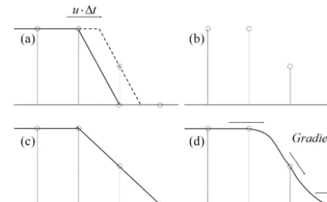
Figure 1.The principle of CIP method:(a)the solid line is the initial profile and the dashed line is an exact solution after ad-vection;(b)discretized points after advection;(c)linearly interpo-lated;(d)interpolated using CIP method.
2.2 The fractional step approach
A fractional step approach is applied to solve the time inte-gration of the governing Eqs. (1) and (2). The first step is to calculate the advection term, neglecting the diffusion term and pressure term, as Eq. (5) shows.
∂u
∂t +(u· ∇)u=0 (5)
A CIP method is employed to solve Eq. (5). The second step is to solve the diffusion term by a central difference scheme:
u∗∗−u∗
1t =
µ ρ∇
2u+F, (6)
whereu∗is the solution of Eq. (5), andu∗∗is the solution to calculate in this step.
The final step is the coupling of the pressure and velocity by considering Eq. (1):
∇ ·
1 ρ∇p
n+1
= 1
1t∇ ·u
∗∗
, (7)
un+1=u∗∗−1t
ρ ∇p
n+1. (8)
Equation (7) is solved by a successive over-relaxation (SOR) method. More details can be found in our previous works (Zhao et al., 2016a, b).
The free surface is captured by a THINC/SW scheme, which is based on the principles of the VOF method. The solid boundary is treated by an IBM (Peskin, 1973).
2.3 CIP method
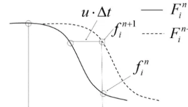
Figure 2.CIP scheme as a kind of semi-Lagrangian method.
the transportation equation of its spatial gradientg=∂f/∂x
are used (seen in Fig. 1).
To explain the steps of the CIP method, we take the fol-lowing 1-D advection equation as an example.
∂f ∂t +u
∂f
∂x =0 (9)
By differentiating Eq. (9) with respect tox, we have the equa-tion of the spatial derivative:
∂g ∂t +u
∂g ∂x = −g
∂u
∂x, (10)
whereg=∂f/∂x. For simplicity, we assume a constant ad-vection velocity. Then Eq. (10) has the same form as Eq. (9). For the case ofu> 0, we approximate a profile forfninside the upwind cell [xi−1,xi] as
Fin(x)=ai(x−xi)3+bi(x−xi)2+ci(x−xi)+di. (11) The spatial gradient offncan be written as
Gni(x)=ai(x−xi)2+bi(x−xi)+ci. (12) As shown in Fig. 2, the profile at the time stepn+1 is ob-tained by shifting the profile with−u·1t; i.e. the time evo-lution of the functionf andgcan be obtained by using the following Lagrangian invariants.
fin+1=Fin(xi−u·1t ) (13)
gin+1=Gni(xi−u·1t ) (14)
Therefore we call the CIP scheme a semi-Lagrangian method.
The four unknown coefficients in Eq. (11) can be deter-mined by using known quantitiesfin,fin−1,ginandgin−1:
ai =
gin−gin 1x2 −
2 fin−fin−1 1x3 , ci=g
n i,
bi =
2gni +gni
1x −
3 fin−fin−1
1x2 , di=f n i .
(15)
By introducing the spatial gradient of variable f, CIP can provide a third-order interpolation function in a single grid. Compared to traditional upwind schemes, CIP method has not only sub-cell resolution but also compact high-order structure.
2.4 THINC/SW scheme
The THINC/SW scheme, first put forward by Xiao et al. (2011), is used for free-surface capturing of incom-pressible flows. Some test examples have indicated that the scheme has the features we need, such as mass conservation and a lack of oscillation (Ji et al., 2013). The basic idea of THINC/SW is that, for the profile of a volume functionϕ(0
≤ϕ≤1), a hyperbolic tangent function with adjustable pa-rameter is used to interpolate inside an upwind cell, which is shown as follows:
χx,i= α
2
1+γtanh
β x−x
i−1/2
1xi
−δ
, (16)
whereα,γ,δandβare parameters to be specified.αandγ
are used to avoid interface smearing and are given by
α=
φi+1 if φi+1≥φi−1
φi−1 otherwise, (17)
γ=
1 if φi+1≥φi−1
−1 otherwise. (18)
Parameterδis used to determine the middle point of the hy-perbolic tangent function and is solved by
1
1xi xi+1/2
Z
xi−1/2
χi(x)dx=φ n
i. (19)
Parameter β determines the steepness of the jump in the interpolation function varying from 0 to 1. In traditional THINC, a constantβ=3.5 is usually used that may result in ruffling the interface, which aligns nearly in the direction of the velocity. To avoid this problem, in THINC/SW,β is determined adaptively according to the orientation of the in-terface. In a 2-D case,β can be written as
βx=2.3|nx| +0.01 βy=2.3|ny| +0.01.
(20)
3 Simulation set-up 3.1 Initial condition
In this section, 2-D numerical wave tanks, including incident waves and geographies, are introduced. Simulation cases are divided into two categories according to different parameters and purposes.
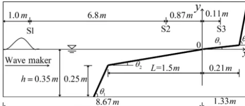
Figure 3. Schematic diagram of Tank 1. tanθ1=25/17, tanθ2= 1/15 and tanθ3=1/30.
fixed at 0.35 m, so that the still-water shoreline is located at the starting point of the beach. This point is regarded as the original point of this tank to determine other positions mentioned in this paper. Tank 1 is used for verifying the ac-curacy of our model and investigating cliff slope gradient and incident wave height, which may influence the tsunami am-plification factor. Five cliff slopes are tested:θ4=14, 21.67, 39.33, 49 and 79◦. Four incident wave heights are consid-ered:H=0.025, 0.035, 0.045 and 0.055 m. A solitary wave is used as an analogue of tsunami in the numerical modelling. S1–3 in Fig. 3 are three gauges of water elevation, located atx= −7.67,−0.87 and 0.11 m, respectively. Outcomes of S1–3 are used for the comparison between numerical results and experimental data (Sim, 2017). Besides, six gauges of water elevation are employed to calculate the tsunami am-plification factor, fixed atx=0.0, 0.06, 0.11, 0.13, 0.16 and 0.21 m (not drawn in Fig. 3).
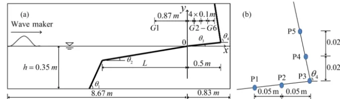
The second simulations utilize Tank 2, similar to Tank 1 except for slight differences, as shown in Fig. 4a. In this tank, the still-water shoreline also lies on the starting point of the beach, which is the original point of this tank. Four gentle submarine slopes (representing the continental shelf) of dif-ferent lengths are used:L=0.764, 1.528, 2.292 and 3.056 m. Three incident wave heights are performed,H=0.04, 0.05, 0.06 m. Two kinds of cliff, a normal cliff ofθ4=80.02◦and a toe-eroded cliff ofθ4=91.91◦, are considered. Six gauges of water elevation are employed to record the waveform evolu-tion, located atx= −0.87, 0.0, 0.1, 0.2, 0.3, 0.4 m. Five pres-sure sensors are arranged near the toe of the cliff, as shown in Fig. 4b. The scales of these two kinds of wave tanks are same to the previous works of Huang et al. (2013), Sim et al. (2015) and Sim (2017).
In this work, considerable attention will be paid to Tank 2. It is necessary to number the simulated cases in Tank 2 to avoid confusion, as shown in Table 1.
3.2 Numerical wavemaker
By declaring a velocity of water particle in the left-most grid and assigning it a value from laboratory wave-paddle
veloc-ity, a numerical paddle wavemaker is set at the left side of wave tank (Figs. 3 and 4a).
For a solitary wave, the approximate solution of wave profile near the wave paddle can be described as follows (Boussinesq, 1872):
η=Hsec h2 "r
3H
4h3(ct−ξ ) #
, (21)
c=pg(h+H ), (22)
whereH,h,candξ are the amplitude of the solitary wave, still-water depth, wave celerity and wave-paddle trajectory, respectively.
The wave-paddle velocity can be calculated as
u1(ξ, t )= dξ
dt. (23)
For a long wave, the depth-averaged horizontal velocity of water particle derived from continuity equation is expressed as (Mei, 1983)
u2(x, t )=
cη(x, t )
h+η(x, t ). (24)
The horizontal water particle velocity adjacent to the paddle is equal to the wave-paddle velocity, which means that when
x=ξ in Eq. (21),u1=u2.
Using Eqs. (21), (23) and (24), wave-paddle trajectory can be derived as an implicit expression:
ξ(t )=
r 4H
3hhtanh "r
4H
3h3(ct−ξ ) #
. (25)
The stroke length of a wave paddle can be calculated as
S=ξ(∞)−ξ(−∞)=
r 16H
3h h. (26)
In theory, a period of solitary wave is infinite. In the applica-tion, it can be approximately defined as follows:
tanh "r
4H
3h3 cT 2 − S 2 #
=0.999, (27)
T =2
c s
4h3
3H
3.8+H
h
. (28)
The water particle velocity imposed in the left-most grid can be given by
u(t )= cη(ξ, t )
h+η(ξ, t )0≤t≤T . (29)
In our model, the left-most grid is not moveable as the labo-ratory wave paddle is, and Eq. (24) should be modified. By some numerical tests, it is finally determined as
u(t )=c[2η(ξ(t ), t )−η(ξ(0), t )]
Figure 4.Schematic diagram of Tank 2. tanθ1=1.38, tanθ2=0.08 and tanθ3=0.02.
Table 1.Summary of basic parameters calculated in Tank 2.
Case θ4=80.02◦ θ4=80.02◦ θ4=80.02◦ θ4=91.91◦ θ4=91.91◦ θ4=91.91◦
H=0.04 m H=0.05 m H =0.06 m H=0.04 m H=0.05 m H =0.06 m
L=0.764 m 1 5 9 13 17 21
L=1.528 m 2 6 10 14 18 22
L=2.292 m 3 7 11 15 19 23
L=3.056 m 4 8 12 16 20 24
4 Numerical result 4.1 Model validation
To verify the accuracy of our model, numerical results from one of the cases in Tank 1 are compared with available ex-perimental data (Sim, 2017). The incident wave height and the cliff slope gradient of this case are H=0.055 m and
θ4=79◦, respectively. A variable grid is used for the com-putation, in which the grid points are concentrated near the free surface and the topography. Three non-uniform grids are used to perform a grid refinement test. The grid quantity and the minimum grid size are shown in Table 2.
Figure 5 concerns the predicted time series of water el-evations at locations S1–3, and the physical measurements (Sim, 2017) are also presented for comparison. Figure 5a illustrates the comparison results at S1. It can be observed that wave has not reached the topography, so that the wave-form has not transwave-formed excessively and is similar to the original waveform. Good general agreement is found for all computations. The relative wave height at S1 is 1.0 m, which reveals the accuracy of the target incident wave. Figure 5b shows the results at S2, x= −0.87 m. This gauge point is in the area of the gentle submarine slope, and shoaling hap-pens when waves propagate here. It can be seen from Fig. 5b that the wave front face becomes steep and the back face be-comes gentle, which means wave asymmetry appears. Re-sults of three grids are in good agreement with experimen-tal data. Figure 5c is the most significant among these three graphs because the gauge station of this graph is located in the front of the cliff, where the flow field is extremely com-plex. Waves rush from the coastline in the form of a water jet. Then, the water jet impacts the cliff, accompanied by
high pressure acting on the toe of cliff. Great acceleration is produced by the impact, making the water run up on the cliff. Under the influence of gravity, water finally falls back and a large quantity of air is entrained in water when back-flow interacts with the incident back-flow. The velocities of water particles fluctuate violently due to the water–cliff interaction and the drastic water–air mixing. The intense spray of wa-ter makes it hard to measure the wawa-ter elevation with a wave gauge. Hence, Sim (2017) employed three HD Pro c910 web cameras to observe wave transformation in addition to the Ultralab sensors. Data of video recordings from Sim (2017) are also presented in Fig. 5c, marked by×. It can be seen from Fig. 5c that the crest value of video data is 18 % smaller than the value of sensor data, which reveals that it is hard to determine the true trace of water surface in such a complex condition. The result of the fine grid is between the result of video data and sensor data, the result of the middle mesh is similar to the video data, and the result of the coarse mesh is 3 % smaller than video data. In general, our model shows a good performance in this verifiable example, even when the flow regime is extremely unstable. More verification of our model can been found in Zhao et al. (2014). However, as the coarse grid has a slight underestimation and the fine grid has low time efficiency, the middle grid will be adopted to com-plete the remaining case studies.
4.2 The tsunami amplification factor in Tank 1
Figure 6 describes the results of the tsunami wave amplifi-cation factor in Tank 1. The tsunami amplifiamplifi-cation factor is defined as a ratio of the local tsunami height to the tsunami height at a reference location. The vertical coordinates are
Table 2.Parameter of three sets of grids (Unit: m).
Horizontal Vertical Horizontal Vertical grid quantity grid quantity minimum grid minimum grid
Coarse grid 826 220 0.008 0.0022 Middle grid 970 320 0.005 0.0015 Fine grid 1228 468 0.003 0.0008
Figure 5.Time series of experimental data and predicted water elevations using different grids:(a)S1,(b)S2 and(c)S3.
reference wave height at a reference locationxr. The refer-ence location in the present study isxr= −0.87 m (same as Sim, 2017), and the reference wave heightHris provided by our numerical model. From the results in Fig. 6, it is observed that there is a critical cliff slope of aboutθ4=45◦. When cliff slope is gentler than the critical value, the tsunami wave am-plification factor increases with the increase of the cliff slope gradient. When the slope is steeper than the critical slope, the effect of the cliff slope gradient becomes insignificant. This result is similar to Sim (2017). As for the influence of inci-dent wave height, it can be found in Fig. 6e and f, of which the wave gauges are close to the cliff. When the cliff slope is gentle, close toθ4=22◦, the tsunami amplification factor increases with the decrease of the incident wave height. As the cliff slope becomes steeper, the effect of different inci-dent waves, negligible at first, becomes important. The crit-ical cliff slope is aboutθ4=45◦. It is noteworthy that under the condition of steep cliff, the tsunami amplification fac-tor increases with the increase of the incident wave height, in contrast to the gentle cliff. A possible reason for this contrary phenomenon is that the velocity of water particles in the high wave is higher, which allows the high wave to more easily run up on the cliff. Thus, when the cliff slope is gentle, the water of a high wave rushes along the cliff and reaches a rearward area, but water of a small wave accumulates at the front of
cliff. Then, as the cliff slopes becomes steeper, the so-called rearward area becomes hard to reach for the high wave. This change allows the high wave to accumulate water in the area of these two gauge stations. Moreover, the tsunami amplifi-cation factor at these two stations keeps increasing with the increase of the cliff slope angle for a given incident wave, whether or not the cliff is steeper or gentler than 45◦. Hence, the presence of a cliff does amplify the water elevations on the beach. The influence is particularly evident for the high wave. In the present study, the largest tsunami amplification factor is 2.86, as shown in Fig. 6f. It is similar to the result of Sim (2017), which has a value of 2.8.
Figure 6.Wave amplification factors,Hm/Hr, of different cliffs:(a)x=0.0 m,(b)x=0.06 m,(c)x=0.11 m,(d)x=0.13 m,(e)x=0.16 m and(f)x=0.21 m.
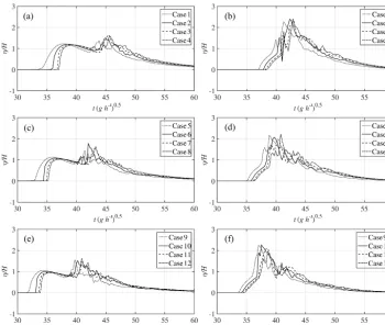
wave is higher than the incident wave. As for Fig. 7b, d and f, when the wave gauges are close to the cliff, it is hard to dis-tinguish the incident and reflected wave. The superposition of incident and reflected wave makes the crest much higher than the results of Fig. 7a, c and e. The effect of initial wave height and length of gentle submarine slope is not clear in Fig. 7 and will be further studied here. The time-series re-sults of cases 13–24 are similar to cases 1–12, which are not shown here.
4.4 Relative wave height in front of the cliff in Tank 2 Wave heights at five gauges in Tank 2, x=0, 0.1, 0.2, 0.3 and 0.4 m, are shown in Fig. 8. The predicted wave height is normalized to the incident wave height,H. The trend line is also presented as the black lines in Fig. 8. In Fig. 8a and b, the maximum relative wave heights are greater than 2.5, and the gradients of trend lines are 2.22 and 2.16, respectively. In
rela-Figure 7.Time series of relative wave elevation in Tank 2:(a),(c)and(e)x=0 m;(b),(d)and(f)x=0.4 m.
tive wave height near the cliff. It reveals a moderate surface wave magnitude, which may cause enormous destruction in near-shore areas.
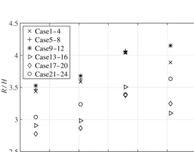
4.5 Wave run-up on the cliff in Tank 2
Figure 9 displays the wave run-up on the cliff in Tank 2; different lengths of gentle submarine slope are compared. The predicted run-up is normalized to the incident wave height, H. It can be seen in Fig. 9 that there is a criti-cal length of gentle submarine slope of aboutL=2.292 m. WhenL< 2.292 m, with a given cliff, the relative wave run-up increases as the length of gentle slope increases. WhenL
goes over the critical length 2.292 m, the wave run-up fluctu-ates. WhenL> 2.292 m, for both normal cliff and toe-eroded cliff, run-up of the case H=0.04 m decreases, but results of the caseH=0.06 m still increase with the increase of the gentle slope length. Moreover, for casesH=0.05 m, the nor-mal cliff results in an increase and the toe-eroded cliff gives an opposite result. It reveals that the critical value relates to both the incident wave height and the inclination of a cliff. In contrast, the run-up on a normal cliff is higher than on toe-eroded cliff. The maximum relative run-up on a normal cliff reaches up to 4.2. The reason for this is that the inclination of normal cliff is accordant with the direction of the incident wave, while the toe-eroded cliff is contrary. Waves can easily climb up on the normal cliff and regurgitate slowly along the
cliff. As for the toe-eroded cliff, a wave reflects on the cliff and some of the water can run up on the cliff; finally, under the action of gravity, water falls back earlier.
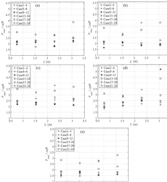
4.6 Impact pressure analysis in Tank 2
Figure 10 shows the time histories of impact pressure on the cliff at two pressure sensors, P3 and P4. The detailed locations of pressure sensors are shown in Fig. 4b. Fig-ure 10a, c, e, g, i and k give the predicted results at lo-cation P3, and the results at lolo-cation P4 are shown in Fig. 10b, d, f, h, j and l. The recorded pressure is normal-ized to the hydrostatic pressure due to incident wave ampli-tude,ρgH. The peak pressure can be divided into two cate-gories, the early peak and the later peak, which are caused by the directly impact and backflow, respectively. It is obvious that the high incident wave height is beneficial to the appear-ance of early peak. Once the early peak appears, it is much larger than the later peak. In the cases of small incident wave height, only the later peak is observed at both measurement points. In the action period, besides the pressure peak, the main scope of relative pressure ranges from 1.0 to 2.5.
Figure 8. Maximum relative wave height in front of the cliff in Tank 2: (a) and (b) H=0.04 m; (c) and (d) H=0.05 m; (e)and(f)H =0.06 m.
Figure 9.Wave run-up on the cliff.
cliff affects the appearance of the pressure peak. Under the condition of a toe-eroded cliff, the generation of pressure peak is frequent. As for the normal cliff, the pressure peak is rare, but it can be significantly large once it appears. In ad-dition, the pressure peak is found to be related to the length of gentle submarine slopeL. WhenLis small, it is easier for a small wave to generate an extreme pressure, which may be caused by backflow; whenLis large, a high wave tends to generate an extreme pressure, which is probably caused by the direct wave impact.
Figure 12 demonstrates the snapshots of the pressure dis-tribution at different time instances. Two typical cases of a normal cliffθ4=80.02◦ (case 12) and a toe-eroded cliff
Figure 11.Maximum impact pressure at five measuring points.
tion of pressure sensor P4 (Figs. 12a and b). Because of the cliff, the wave front is deviated and is deflected to a water jet along the cliff. As the water runs up the cliff, it is slowed down by gravity. Also it seems that the pressure impacting on the cliff has been decreased a little (Figs. 12c and d). More-over, significant water splashing of small water droplets can be observed, contributed from our numerical model. Finally, the water falls back from the cliff due to gravity. This causes the formation of a backward plunging backflow hitting the underlying water, entrapping air. At this stage, extreme pres-sure appears again and the scope is large, mainly on the beach in front of the cliff. Due to the cliff inclination angle effect, the detailed water flow characteristic on the toe-eroded cliff is found to be different from that on the normal cliff. When the wave propagates along the gentle slope and hits the cliff, the water front horizontal velocity is changed upward along the cliff, as shown in Figs. 12a and b. As time goes on, the wave run-up on the toe-eroded cliff deviates from the cliff due to gravity (Fig. 12d), which will cause a violent plunging breaker onto the underlying water (Fig. 12f). While for a
Figure 12.Snapshots of impact pressure distribution in front of the cliff.(a, c, e)case12;(b, d, f)case24.
5 Discussion
The tsunami amplification factor is essentially a kind of rel-ative wave height that normalized to the height at a reference location. The interesting result in the present work is as fol-lows. In Tank 1, we analyse the tsunami amplification factor near the steepest cliff and find that it increases with the ini-tial wave height (as Fig. 6e and f shown). However, in Tank 2, when the gauge is close to the normal cliff, the relative wave height decreases as the initial wave height increases (seen in Fig. 8a, c and e). It seems that the results of Tank 1 and Tank 2 are contradictory. One of the possible explanations is the influence of the beach. The most significant difference between Tank 1 and 2 is the length of beach. The effect of beach can be simply summed up as follows. The longer the beach is, the more energy is lost before wave impact. The beach is also an area for the mixing of incident and reflected wave; for a large wave, which requires a long area for mix-ing when the beach is not long enough, the drastic mixmix-ing will occur under the coastal line. The details of the beach ef-fect, including process of mixing and energy dissipation, are a meaningful research subject for future work.
As for the run-up in Tank 2, a critical length of gentle submarine slope is found for some cases. Before the wave gets across the coastal line, gentle submarine slope facilitates wave deformation and energy focus. A proper slope helps a wave to adequately prepare before it touches the cliff. When the slope is too long, as the wave reaches the shore line it may have broken or be on the verge of breaking, which makes en-ergy dissipate ahead of time. However, the optimum length is affected by several factors such as initial wave height and cliff slope; this is why there is no critical value found in some cases. From the present work, it is reasonable to specu-late that higher initial waves require longer, gentle submarine slopes to achieve the critical value. This can be connected to the analysis of Fig. 11 that whenL is small, a small wave
generates extreme pressure, and when L becomes large, a high wave tends to generate extreme pressure. In contrast, a normal cliff also enlarges the critical value compared to toe-eroded cliff. The complicated relationship between these factors needs an even deeper investigation.
The present work is only a start as the understanding of tsunami inundation needs to be expanded upon and quanti-fied.
6 Conclusions
In this study, tsunami wave impact and run-up in the presence of submarine gentle slopes and a coastal cliff are investigated numerically using a CIP-based model. Numerical results are initially compared with available experimental data and the good agreement revealed the ability of our model to solve the complex flow field, such as wave breaking, water–air mixing and violent impact. The results can be summarized as fol-lows.
1. The gradient of cliff slope has a critical value about 45◦; different characteristics of tsunami amplification factor have been found when the angle is greater or smaller than 45◦.
2. The length of gentle submarine slope influences the tsunami wave run-up and has a critical value of about
L=2.292 m in this study for some cases.
3. When wave transforms near the cliff, the cases with small incident wave height have a larger relative wave height, which means a devastating tsunami may be caused by a moderate source.
5. There are two opportunities for the appearance of pres-sure peak during the process of tsunami wave run-up and impact. One is the direct impacting pressure when tsunami waves first hit the coastal cliff, and the other is caused by the backflow from the cliff after run-up with a widely affected area.
The present study gives the history of tsunami evolution from open sea to coastal area, which is rare in field study. Several topographies and different incident waves have been consid-ered. Comparing with the SWE result, which may under-rate and need amendment, the present results can simulate the tsunami in near-shore areas more accurately. The present model is helpful for tsunami forecast, danger prediction and post-disaster analysis. Furthermore, combined with geology knowledge, the earthquake source magnitude and generation location can be determined.
Data availability. No data sets were used in this article.
Competing interests. The authors declare that they have no conflict of interest.
Acknowledgements. This work was financially supported by the National Natural Science Foundation of China (grant nos. 51479175, 51679212 and 51409231) and Zhejiang Provincial Natural Science Foundation of China (grant no. LR16E090002).
Edited by: M. Gonzalez
Reviewed by: two anonymous referees
References
Baptista, A. M., Priest, G. R., and Murty, T. S. M.: Field sur-vey of the 1992 Nicaragua tsunami, Mar. Geod., 16, 169–203, doi:10.1080/15210609309379687, 1993.
Boussinesq, J.: Théorie des ondes et des remous qui se propagent le long d’un canal rectangulaire horizontal, en communiquant au liquide contenu dans ce canal des vitesses sensiblement pareilles de la surface au fond, Journal de Mathématiques Pures et Ap-pliquées, 17, 55–108, 1872.
Dao, M. H., Xu, H., Chan, E. S., and Tkalich, P.: Modelling of tsunami-like wave run-up, breaking and impact on a vertical wall by SPH method, Nat. Hazards Earth Syst. Sci., 13, 3457–3467, doi:10.5194/nhess-13-3457-2013, 2013.
Dawson, A. G.: Geomorphological effects of tsunami run-up and backwash, Geomorphology, 10, 83–94, doi:10.1016/0169-555X(94)90009-4, 1994.
Fu, Y., Zhao, X., Cao, F., Zhang, D., Cheng, D., and Li, L.: Numer-ical simulation of viscous flow past an oscillating square cylin-der using a CIP-based model, J. Hydrodyn., Ser. B, 29, 96–108, doi:10.1016/S1001-6058(16)60721-7, 2017.
Goto, K., Chagué-Goff, C., Fujino, S., Goff, J., Jaffe, B., Nishimura, Y., Richmond, B., Sugawara, D., Szczuci´nski, W., Tappin, D. R.,
Witter, R. C., and Yulianto, E.: New insights of tsunami haz-ard from the 2011 Tohoku-oki event, Mar. Geol., 290, 46–50, doi:10.1016/j.margeo.2011.10.004, 2011.
Gupta, V. K., Srikanth, K., and Punekar, H.: Improvements in free surface flow numerics using coupled vof and pseudo transient solver[C]//High Performance Computing Workshops (HiPCW), 2016 IEEE 23rd International Conference on. IEEE, avail-able at: http://ieeexplore.ieee.org/stamp/stamp.jsp?arnumber= 7837055 (last access: 5 May 2017), 100–105, 19–22 Decem-ber 2016.
Hu, C. and Kashiwagi, M.: Two-dimensional numerical simulation and experiment on strongly nonlinear wave–body interactions, J. Mar. Sci. Technol., 14, 200–213, doi:10.1007/s00773-008-0031-4, 2009.
Hirt, C. W. and Nichols, B. D.: Volume of fluid (VOF) method for the dynamics of free boundaries, J. Comput. Phys., 39, 201–225, doi:10.1016/0021-9991(81)90145-5, 1981.
Ha, T., Shim, J., Lin, P., and Cho, Y. S.: Three-dimensional nu-merical simulation of solitary wave run-up using the IB method, Coast. Eng., 84, 38–55, doi:10.1016/j.coastaleng.2013.11.003, 2014.
Huang, Z., Wu, T., Chen, T., and Sim, S. Y.: A possible mechanism of destruction of coastal trees by tsunamis: A hydrodynamic study on effects of coastal steep hills, Journal of Hydro-environment Research, 7, 113–123, doi:10.1016/j.jher.2012.06.004, 2013.
Ji, Q., Zhao, X., and Dong, S.: Numerical study of violent impact flow using a CIP-based model, J. Appl. Math., 2013, 4819–4828, doi:10.1155/2013/920912, 2013.
Kawasaki, K. and Suzuki, K.: Numerical simulation of tsunami run-up and inundation employing horizontal two-dimensional model based on cip method, Procedia Engineering, 116, 535– 543, doi:10.1016/j.proeng.2015.08.323, 2015.
Lin, P., Cheng, L., and Liu, D.: A two-phase flow model for wave-structure interaction using a virtual bound-ary force method, Comput. Fluids, 129, 101–110, doi:10.1016/j.compfluid.2016.02.007, 2016.
Liu, P. L. F., Lynett, P., Fernando, H., Jaffe, B. E., Fritz, H., Higman, B., Morton, R., Goff, J., and Synolakis, C.: Observations by the international tsunami survey team in Sri Lanka, Science, 308, 1595–1595, doi:10.1126/science.1110730, 2005.
Liu, P. L. F., Synolakis, C., and Yeh, H.: Report on the International Workshop on Long-Wave Run-up, J. Fluid Mech., 229, 675–688, doi:10.1017/S0022112091003221, 1991.
Mei, C. C.: The applied dynamics of ocean waves, John Wiely & Sons, New York, 1983.
Markus, D., Arnold, M., Wüchner, R., and Bletzinger, K. U.: A Vir-tual Free Surface (VFS) model for efficient wave–current CFD simulation of fully submerged structures, Coast. Eng., 89, 85– 98, doi:10.1016/j.coastaleng.2014.04.004, 2014.
Malgarinos, I., Nikolopoulos, N., and Gavaises, M.: Coupling a lo-cal adaptive grid refinement technique with an interface sharpen-ing scheme for the simulation of two-phase flow and free-surface flows using VOF methodology, J. Comput. Phys., 300, 732–753, doi:10.1016/j.jcp.2015.08.004, 2015.
Monecke, K., Finger, W., Klarer, D., Kongko, W., McAdoo, B. G., Moore, A. L., and Sudrajat, S. U.: A 1,000-year sediment record of tsunami recurrence in northern Sumatra, Nature, 455, 1232– 1234, doi:10.1038/nature07374, 2008.
Quiyoom, A., Ajmani, S. K., and Buwa, V. V.: Role of free surface on gas-induced liquid mixing in a shallow vessel, AIChE Journal, 1–17, doi:10.1002/aic.15697, 2017.
Oliveira, T. C. A., Sanchez-Arcilla, A., Gironella, X., and Madsen, O. S.: On the generation of regular long waves in numerical wave flumes based on the particle finite element method, J. Hydraul. Res., 1–19, doi:10.1080/00221686.2016.1275047, 2017. Peskin, C. S.: Flow patterns around heart valves, Lecture Notes in
Physics, 10, 214–221, doi:10.1007/BFb0112697, 1973. Rosser, N. J. and Petley, D. N.: Terrestrial laser scanning for
moni-toring the process of hard rock coastal cliff erosion, Q. J. Eng. Geol. Hydroge., 38, 363–376, doi:10.1144/1470-9236/05-008, 2005.
Satake, K.: Mechanism of the 1992 Nicaragua tsunami earthquake, Geophys. Res. Lett., 21, 2519–2522, doi:10.1029/94GL02338, 1994.
Sim, S. Y.: Run-up related to onshore tsunami flows, PhD Thesis, Nanyang Technological University, Singapore, 2017.
Sim, S. Y. and Huang, Z.: An experimental study of tsunami amplification by a coastal cliff, J. Coastal Res., 32, 611–618, doi:10.2112/JCOASTRES-D-15-00032.1, 2015.
Sonobe, T., Okubo, K., Tagawa, N., and Tsuchiya, T.: A novel numerical simulation of acoustic Doppler effect using CIP-MOC method, J. Acoust. Soc. Am., 140, 3249–3249, doi:10.1121/1.4970280, 2016.
Stephenson, W. J. and Naylor, L. A.: Within site geological contin-gency and its effect on rock coast erosion, J. Coastal Res., SI64, 831–835, 2011.
Takewaki, H., Nishiguchi, A., and Yabe, T.: Cubic interpo-lated pseudo-particle method (CIP) for solving hyperbolic-type equations, J. Comput. Phys., 61, 261–268, doi:10.1016/0021-9991(85)90085-3, 1985.
Tanaka, R., Nakamura, T., and Yabe, T.: Constructing exactly con-servative scheme in a non-concon-servative form, Comput. Phys. Commun., 126, 232–243, doi:10.1016/S0010-4655(99)00473-7, 2000.
Vicinanza, D., Salerno, D., and Buccino, M.: Structural Response of Seawave Slot-cone Generator (SSG) from Random Wave CFD Simulations[C], The Twenty-fifth International Offshore and Po-lar Engineering Conference, International Society of Offshore and Polar Engineers, 21–26 June 2015.
Xiao, F., Honma, Y., and Kono, T.: A simple algebraic interface cap-turing scheme using hyperbolic tangent function, Int. J. Numer. Meth. Fl., 48, 1023–1040, doi:10.1002/fld.975, 2005.
Xiao, F., Ii, S., and Chen, C.: Revisit to the THINC scheme: a sim-ple algebraic VOF algorithm, J. Comput. Phys., 230, 7086–7092, doi:10.1016/j.jcp.2011.06.012, 2011.
Youngs, D. L.: Time-dependent multi-material flow with large fluid distortion, Numerical Methods for Fluid Dynamics, 24, 273–285, 1982.
Yokoi, K.: A practical numerical framework for free surface flows based on CLSVOF method, multi-moment methods and density-scaled CSF model: Numerical simulations of droplet splashing, J. Comput. Phys., 232, 252–271, doi:10.1016/j.jcp.2012.08.034, 2013.
Yokoi, K.: Efficient implementation of THINC scheme: a simple and practical smoothed VOF algorithm, J. Comput. Phys., 226, 1985–2002, 2007.
Yasuhara, K., Murakami, S., Kanno, Y., and Wu, Z.: Fe analysis of coastal cliff erosion due to ocean wave assailing, First Interna-tional Conference on Scour of Foundations, 2002.
Zhao, X., Cheng, D., Zhang, D., and Hu, Z.: Numerical study of low-Reynolds-number flow past two tandem square cylinders with varying incident angles of the downstream one using a CIP-based model, Ocean Eng., 121, 414–421, doi:10.1016/j.oceaneng.2016.06.005, 2016a.
Zhao, X., Gao, Y., Cao, F., and Wang, X.: Numerical modeling of wave interactions with coastal structures by a constrained in-terpolation profile/immersed boundary method, Int. J. Numer. Meth. Fl., 81, 265–283, doi:10.1002/fld.4184, 2016b.