Estimation of open channel flow parameters by using optimization techniques

(1)

IJEDR1702179 International Journal of Engineering Development and Research (www.ijedr.org) 1049

Estimation of open channel flow parameters

by using optimization techniques

1_{Ebissa G. K.,}2_{Dr. K. S. Hari Prasad}

Department of Civil Engineering, Indian Institute of Technology Roorkee

ABSTRACT: Open channel flow parameter estimation is an inverse problem, which involves

the prediction of a function within a domain, given an error criterion with respect to a set of

observed data. Various numerical methods have been developed to estimate open channel flow

parameters. For this study, Genetic Algorithm optimization technique is selected. Because of its

inherent characteristics, Genetic Algorithm optimization technique avoids the subjectivity, long

computation time and ill-posedness often associated with conventional optimization techniques.

The present study involves estimation of open channel flow parameters having different bed

materials invoking data of Gradual Varied Flow (GVF). Use of GVF data facilitates estimation

of flow parameters. The necessary data base was generated by conducting laboratory

experiments in Hydraulics Lab of civil Engineering at IIT Roorkee. In the present study, the

efficacy of the Genetic Algorithm (GA) optimization technique is assessed in estimation of open

channel flow parameters from the collected experimental data. Computer codes are developed to

obtain optimal flow parameters Optimization Technique. Applicability, Adequacy & robustness

of the developed code are tested using sets of theoretical data generated by experimental work.

Estimation of Manning’s Roughness coefficient from the collected experimental work data by

using Manning’s equation & GVF equation were made.

The model is designed to arrive at such values of the decision variables that permit minimized

mismatch between the observed & the computed GVF profiles. A simulation model was

developed to compute GVF depths at preselected discrete sections for given downstream head

and discharge rate. This model is linked to an optimizer to estimate optimal value of decision

variables. The proposed model is employed to a set of laboratory data for three bed materials (i.e,

d50=20mm, d50=6mm and lined concrete). Application of proposed model reveals that optimal

value of fitting parameter ranges from 1.42 to 1.48 as the material gets finer. This value differs

(2)

different bed conditions of experimental channel appear to be higher than the corresponding

reported /Strickler’s’ estimates.

Key Words:- Open channel flow parameters, GVF, parameter estimation, optimization

techniques, Manning’s roughness coefficient.

INTRODUCTION

Parameter identification techniques have been widely used in the field of hydrology,

meteorology, and oceanography. The issue of parameter identification based on the optimal

control theories in oceanography can be traced from the early work of Bennett and McIntosh

(1982) and Prevost and Salmon (1986). Panchang and O’Brien (1989) carried out early an

adjoint parameter identification for bottom drag coefficient in a tidal channel. Das and Lardner

(1991) estimated the bottom friction and water depth in a two-dimensional tidal flow. Yeh and

Sun (1990) presented an adjoint sensitivity analysis for a groundwater system and identified the

parameters in a leaky aquifer system. Wasantha Lal (1995) used singular value decomposition to

calibrate the Manning’s roughness in one-dimensional (1D) Saint Venant equations. Khatibi et

al. (1997) identified the friction parameter in 1D open channel considering the selection of

performance function and effect of uncertainty in observed data. Atanov et al. (1999) Used the

adjoint equation method to identify a profile of Manning’s n in an idealized trapezoidal open

channel. Ishii (2000) identified a constant Manning’s n in an open channel flow with a movable

bed. Ramesh et al. (2000) solved the inverse problem of identifying the roughness coefficient in

a channel network using the sequential quadratic programming algorithm. Sulzer et al. (2002)

estimated flood discharges using the Levenberg–Marquardt minimization algorithm. For the

parameter identification issues about adjoint methodology in meteorology and oceanography,

one may refer to Ghil and Malanotte-Rizzoli (1991) and Zou et al. (1992).

The identifications of parameters in some cases are hard to achieve due to ill-posedness in the

inverse problems. Chavent (1974) noted instability and nonuniqueness of identified parameters

in the distributed system. Due to the instability, some minimization procedures will lead to

serious errors in the identified parameters and make the identification process unstable. In the

case of nonuniqueness, the identified parameters will differ according to the initial estimations of

(3)

(1998) have pointed out that the problem of uniqueness in parameter identification is intimately

related to identification, which addresses the question of whether it is at all possible to obtain a

unique solution of the inverse problem for unknown parameters. Although there are a lot of

identification procedures available for estimating parameters in mathematical models, none of

them can automatically guarantee stability and uniqueness in the parameter identifications in

diverse engineering problems. It is therefore vital to confirm the performance of these procedures

to find stable ones that can warrant obtaining the optimal solutions. For the present study,

channel roughness is identified by using optimization technique.

Optimization techniques were successfully used by Becker and Yeh (1972, 1972a), Fread and

Smith (1978) and Wormleaton and Karmegam (1984) to identify parameters for regular

prismatic channels having simple cross-sections. These researchers used the same optimization

algorithm (the so-called "Influence Coefficient" Algorithm) which, mathematically, is closely

related to both quasi linearization and the gradient method. Khatibi et al. (1997) used a nonlinear

least square technique with three types of objective function and identified open channel friction

parameters by a modified Gauss-Newton method. Atanov et al. (1999) used Lagrangian

multipliers and a least square errors criterion to estimate roughness coefficients. More recently,

Ding et al. (2004) used the quasi-Newton method to identify Manning’s roughness coefficients in

shallow water flows. Nevertheless, the above studies considered only the case of in-bank flow.

Therefore, there is a need to extend the method to out-bank flow, where flood plain roughness

will obviously have to be considered.

One of the very few studies which dealt with the identification of compound channel flow

parameters is the one by Nguyen and Fenton (2005). In this study, roughness coefficients in the

main channel and flood plains were identified as two different parameters using an automatic

optimization method. The model was applied to Duong River in Vietnam, where roughness

coefficients of the main channel and the flood plain were presented as different constant values

as well as polynomial functions of stage.

Need for the Present Study: From above brief literature review it can be seen that many

(4)

by using optimization techniques. Still more experimental study is required to estimate open

channel flow parameters. The present study investigated for estimation of channel roughness

coefficients for different three types of bed materials (d50=20mm, d50=6mm and lined concrete)

by using optimization method. Also the present study is done to generate and monitor gradually

varied flow profiles corresponding to different bed materials, discharge rates and ponded depths

in the channel by using Crank-Nicolson method to solve the governing differential equation.

In this study the Simplex method is used in an optimization model to estimate the parameters in

the channel.

Objectives: The present study involves estimation of Manning roughness n of a channel having

different channel bed materials invoking data of gradual varied flow (GVF). Use of GVF data

facilitates estimation of depth dependent Manning’s roughness n. the necessary data base was

generated by conducting laboratory experiments. The overlying objective is fulfilled through the

accomplishment of sub objectives listed below.To identify open channel flow parameters by

using Genetic Algorithm optimization Technique, To generate and monitor gradually varied flow

profiles corresponding to different bed materials, discharge and ponded depths and Invoking the

observed data of the GVF profiles and the linked simulation optimization approach to estimates

Manning’s n corresponding to different channel bed materials in the experimental channel, and

hence to calibrate the following composite roughness equation.

METHODS AND MATERIALS

This study was carried out to identify open channel flow parameters by using Genetic Algorithm

optimization technique. Manning’s roughness coefficient and other parameters are estimated for

different bed materials used ( d50 =6mm and 20mm grain size and Lined concrete bed materials).

Also, GVF flow profile is identified. Crank-Nicolson method is used to solve the governing

differential equation.

Parameter optimization technique is used to find the optimal value of coefficient roughness for

three different bed materials. Estimation of roughness coefficient is based on Manning’s

(5)

parameters. This estimation invokes the data of observed GVF profiles and such accounts for

different bed materials with the flow depth. Experimental works was done to several sets of data

monitored in Hydraulics Laboratory of Civil Engineering Department.

Experimental Works

In this chapter, water surface flow profiles corresponding to specific discharges, bed material and

ponded depth have been obtained through experimentation. This chapter includes a detailed

description of experimental setup, adopted procedures and the observations with range of data

obtained for different flow conditions. The experiments for the investigation were carried out in

Hydraulics Laboratory of Civil Engineering Department. IIT-Roorkee, India

Details of Experimental Setup

Flume

A rectangular tilting flume of length 30m, width 0.205m and height 0.50m was used. The bed of

the flume was made up of lined concrete and the other two sides were made up of glass and GI

sheet. Discharge was released through an inlet pipe of 0.010m diameter into the flume. The

entrance of the channel was provided with flow suppressors in order to make the flow stable. In

order to maintain desired depth of water at the downstream of the channel, a tail gate was fitted

at the end of the channel. Water discharging from the tail gate, passed to the sump which was

circulated again through a 15hp centrifugal pump for further experimentation.

Experimental Procedures

The experiments were conducting by adopting the following steps as mentioned below:-

Slope Measurement

All the sets of experiment were performed on a particular slope of the channel. The slope was

measured by using two steel containers connected with a long rubber tube. Both the containers

were placed on the channel bed separated by the rubber tube along the length of the channel. One

of the containers placed at higher elevation was filled with water and simultaneously care was

(6)

amount of time around 24 hours. Then the water levels were measured. The slope of the channel

was computed by using the following formula.

𝑆

_𝑜

=

𝐻1−𝐻2

𝐿

(1)

Where, H2 and H1 is the depth of water in second and first container respectively after

equilibrium is established and L is the distance between the containers.

Based on this formula and obtained data after 24 hours, the bed slope of the channel will be;-

H1=21.5cm=0.215m, H2=7.792cm=0.0792m and distance between the two containers, L=22.7m

Then

, 𝑆

_𝑜

=

𝐻1−𝐻2

𝐿

, 𝑆

𝑜

=

0.215−0.0792

22.7

, 𝑆

𝑜

= 0.00598

Therefore, the bed slope of the channel is 0.00598.

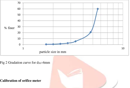
Sieve Analysis

Sieve analysis was performed to determine the particle size of the material used to create

artificial bed roughness. Results of sieve analysis were plotted to investigate the particle size of

the bed material used in the present study. Experiments were conducted on two different bed

materials. First on one rough bed condition having gravel as a bed particle size d50 =20mm,

d50=6mm and then on the smooth condition having lined concrete as bed material. Then, the

gradation curve is plotted as follow:

-20 0 20 40 60 80 100

1 10 100

(7)

Fig 1 Gradation curve for d50=20mm

Fig 2 Gradation curve for d50=6mm

Calibration of orifice meter

Orifice meter was provided in the inlet pipe for the measurement of discharge. Orifice plate was

made up of GI sheet having diameter of 0.06m and the diameter of inlet pipe was 0.10m.

Ultrasonic flow meter was used for the calibration of coefficient of discharge of orifice meter.

Different discharges were noted corresponding to varying head. This result was plotted and the

best fitted line was used (Fig. 3).

0 10 20 30 40 50 60 70

1 10

particle size in mm % finer

0 0.002 0.004 0.006 0.008 0.01 0.012

0 0.05 0.1 0.15 0.2

√H (m)

(8)

Fig. 3 Calibration curve

Cd was calibrated as 0.66. after calibration of Cd of orifice meter, the discharge in the channel

was computed by using the following equation.

𝑄 = 𝐶

_𝑑

𝑎

_𝑜

√2𝑔ℎ (2)

Where, ao is area of orifice plate; g= acceleration due to gravity and h= height of water column.

Measurement of water surface profiles

i) Water was released into the rectangular flume by opening the valve of inlet pipe,

ii) The desired depth of flow was maintained at the downstream end by operating sluice gate

provided at the end of the channel. The depth of water was measured using pointer gauge,

iii) After a while when the flow become steady in the channel and the desired depth was

maintained at the downstream end, the water surface profile was being measured,

iV) Starting from the maintained depth at the downstream end (0.00m), the water surface profile

is measured towards upstream at 21 discrete locations that are 0.00m, 0.20m, 0.70m, 1.20m,

1.70m, 2.20m, 2.70m, 3.70m, 4.70m, 5.70m, 6.70m, 7.70m, 8.70m, 9.70m, 10.70m, 12.70m,

14.70m, 16.70m, 18.70m, 20.70m and 22.70m.

v) The above mentioned steps were repeated for thee different downstream depths, Discharges

rates and bed roughness as mentioned in Table 1

Table 1 Data used for experimental measurement of water surface profiles

Discharge rates

(m3/s)

8.601x10-3 9.233x10-3 9.314x10-3

Downstream depths

(m)

0.25 0.30 0.35

Bed materials

(d50 in mm)

(9)

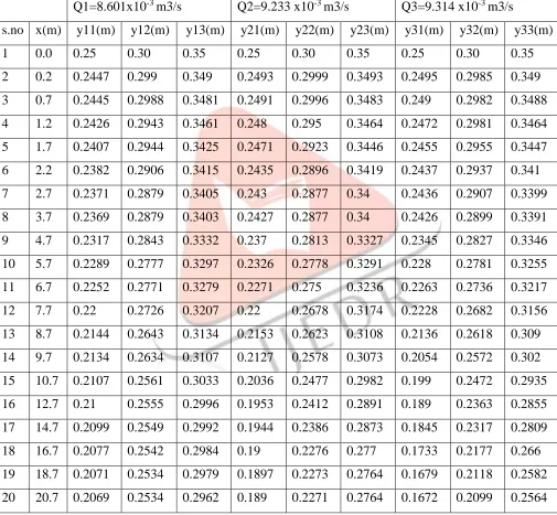
IJEDR1702179 International Journal of Engineering Development and Research (www.ijedr.org) 1057 Collection of data

The data obtained for experimental measured water surface profiles corresponding to different

bed materials is presented in Table 2, 3 and 4 for d50=20mm, d50=6mm and lined concrete

respectively.

Table 2 Observed water surface profiles corresponding to d50=20mm

Q1=8.601x10-3 m3/s Q2=9.233 x10-3 m3/s Q3=9.314 x10-3 m3/s

s.no x(m) y11(m) y12(m) y13(m) y21(m) y22(m) y23(m) y31(m) y32(m) y33(m)

1 0.0 0.25 0.30 0.35 0.25 0.30 0.35 0.25 0.30 0.35

2 0.2 0.2447 0.299 0.349 0.2493 0.2999 0.3493 0.2495 0.2985 0.349

3 0.7 0.2445 0.2988 0.3481 0.2491 0.2996 0.3483 0.249 0.2982 0.3488

4 1.2 0.2426 0.2943 0.3461 0.248 0.295 0.3464 0.2472 0.2981 0.3464

5 1.7 0.2407 0.2944 0.3425 0.2471 0.2923 0.3446 0.2455 0.2955 0.3447

6 2.2 0.2382 0.2906 0.3415 0.2435 0.2896 0.3419 0.2437 0.2937 0.341

7 2.7 0.2371 0.2879 0.3405 0.243 0.2877 0.34 0.2436 0.2907 0.3399

8 3.7 0.2369 0.2879 0.3403 0.2427 0.2877 0.34 0.2426 0.2899 0.3391

9 4.7 0.2317 0.2843 0.3332 0.237 0.2813 0.3327 0.2345 0.2827 0.3346

10 5.7 0.2289 0.2777 0.3297 0.2326 0.2778 0.3291 0.228 0.2781 0.3255

11 6.7 0.2252 0.2771 0.3279 0.2271 0.275 0.3236 0.2263 0.2736 0.3217

12 7.7 0.22 0.2726 0.3207 0.22 0.2678 0.3174 0.2228 0.2682 0.3156

13 8.7 0.2144 0.2643 0.3134 0.2153 0.2623 0.3108 0.2136 0.2618 0.309

14 9.7 0.2134 0.2634 0.3107 0.2127 0.2578 0.3073 0.2054 0.2572 0.302

15 10.7 0.2107 0.2561 0.3033 0.2036 0.2477 0.2982 0.199 0.2472 0.2935

16 12.7 0.21 0.2555 0.2996 0.1953 0.2412 0.2891 0.189 0.2363 0.2855

17 14.7 0.2099 0.2549 0.2992 0.1944 0.2386 0.2873 0.1845 0.2317 0.2809

18 16.7 0.2077 0.2542 0.2984 0.19 0.2276 0.277 0.1733 0.2177 0.266

19 18.7 0.2071 0.2534 0.2979 0.1897 0.2273 0.2764 0.1679 0.2118 0.2582

(10)

21 22.7 0.2031 0.2494 0.2934 0.1872 0.2253 0.2712 0.1511 0.1929 0.2389

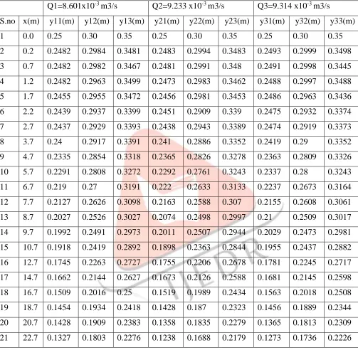
Table 3 Observed water surface profiles corresponding to d50=6mm

Q1=8.601x10-3 m3/s Q2=9.233 x10-3 m3/s Q3=9.314 x10-3 m3/s

S.no x(m) y11(m) y12(m) y13(m) y21(m) y22(m) y23(m) y31(m) y32(m) y33(m)

1 0.0 0.25 0.30 0.35 0.25 0.30 0.35 0.25 0.30 0.35

2 0.2 0.2482 0.2984 0.3481 0.2483 0.2994 0.3483 0.2493 0.2999 0.3498

3 0.7 0.2482 0.2982 0.3467 0.2481 0.2991 0.348 0.2491 0.2998 0.3445

4 1.2 0.2482 0.2963 0.3499 0.2473 0.2983 0.3462 0.2488 0.2997 0.3488

5 1.7 0.2455 0.2955 0.3472 0.2456 0.2981 0.3453 0.2486 0.2963 0.3436

6 2.2 0.2439 0.2937 0.3399 0.2451 0.2909 0.339 0.2475 0.2932 0.3374

7 2.7 0.2437 0.2929 0.3393 0.2438 0.2943 0.3389 0.2474 0.2919 0.3373

8 3.7 0.24 0.2917 0.3391 0.241 0.2886 0.3352 0.2419 0.29 0.3352

9 4.7 0.2335 0.2854 0.3318 0.2365 0.2826 0.3278 0.2363 0.2809 0.3326

10 5.7 0.2291 0.2808 0.3272 0.2292 0.2761 0.3243 0.2337 0.28 0.3243

11 6.7 0.219 0.27 0.3191 0.222 0.2633 0.3133 0.2237 0.2673 0.3164

12 7.7 0.2127 0.2626 0.3098 0.2163 0.2588 0.307 0.2155 0.2608 0.3061

13 8.7 0.2027 0.2526 0.3027 0.2074 0.2498 0.2997 0.21 0.2509 0.3017

14 9.7 0.1992 0.2491 0.2973 0.2011 0.2507 0.2944 0.2029 0.2473 0.2981

15 10.7 0.1918 0.2419 0.2892 0.1898 0.2363 0.2844 0.1955 0.2437 0.2882

16 12.7 0.1745 0.2263 0.2727 0.1755 0.2206 0.2678 0.1781 0.2245 0.2717

17 14.7 0.1662 0.2144 0.2627 0.1673 0.2126 0.2588 0.1681 0.2145 0.2598

18 16.7 0.1509 0.2016 0.25 0.1519 0.1989 0.2434 0.1563 0.2018 0.2508

19 18.7 0.1454 0.1934 0.2418 0.1428 0.187 0.2323 0.1456 0.1889 0.2344

20 20.7 0.1428 0.1909 0.2383 0.1358 0.1835 0.2279 0.1365 0.1813 0.2309

21 22.7 0.1327 0.1803 0.2276 0.1238 0.1688 0.2179 0.1273 0.1736 0.2226

(11)

Q1=8.601x10-3 m3/s Q2=9.233 x10-3 m3/s Q3=9.314 x10-3 m3/s

s.no x(m) y11(m) y12(m) y13(m) y21(m) y22(m) y23(m) y31(m) y32(m) y33(m)

1 0.0 0.25 0.30 0.35 0.25 0.30 0.35 0.25 0.30 0.35

2 0.2 0.2435 0.2953 0.3472 0.2455 0.298 0.3494 0.2474 0.2992 0.348

3 0.7 0.2419 0.2964 0.3474 0.2474 0.2974 0.3493 0.2465 0.2948 0.3527

4 1.2 0.237 0.2941 0.3461 0.2469 0.2887 0.3489 0.2449 0.2889 0.3469

5 1.7 0.2336 0.2918 0.3429 0.242 0.2874 0.344 0.243 0.2966 0.3463

6 2.2 0.2292 0.2911 0.341 0.2338 0.2874 0.3431 0.2429 0.2919 0.3458

7 2.7 0.2282 0.2872 0.3382 0.2319 0.2855 0.3402 0.2428 0.2918 0.3447

8 3.7 0.2198 0.2819 0.3327 0.2301 0.2809 0.3356 0.2359 0.291 0.3436

9 4.7 0.2173 0.2762 0.3272 0.2236 0.2764 0.3311 0.2345 0.2873 0.3363

10 5.7 0.2117 0.2708 0.3227 0.2154 0.2672 0.3265 0.231 0.2747 0.3326

11 6.7 0.2051 0.2651 0.3152 0.2125 0.2615 0.3181 0.2235 0.2671 0.3251

12 7.7 0.1958 0.2559 0.306 0.1986 0.2505 0.3005 0.2061 0.2532 0.3132

13 8.7 0.189 0.2426 0.291 0.1936 0.2463 0.2947 0.1973 0.2491 0.3026

14 9.7 0.1808 0.2327 0.2864 0.1901 0.2399 0.293 0.1955 0.2428 0.2936

15 10.7 0.1718 0.2253 0.2715 0.1811 0.2329 0.2884 0.1856 0.2401 0.2892

16 12.7 0.1654 0.2191 0.2682 0.1619 0.2108 0.2674 0.1673 0.2265 0.2772

17 14.7 0.1571 0.2089 0.2583 0.1547 0.2036 0.263 0.1629 0.2155 0.2759

18 16.7 0.1463 0.2041 0.2564 0.1391 0.1918 0.2458 0.1501 0.1975 0.2664

19 18.7 0.1443 0.201 0.2551 0.1201 0.1765 0.232 0.1439 0.1893 0.241

20 20.7 0.1419 0.1996 0.2537 0.1146 0.1647 0.2185 0.1203 0.1821 0.2276

21 22.7 0.1418 0.1965 0.2506 0.1028 0.1591 0.2148 0.1137 0.1665 0.2146

RESULTS AND DISCUSSION

Simulation Model

The optimization problem posed in the preceding section is solved by employing the linked

optimization problem. This approach would require development of a model for simulation of

(12)

Subsequently this simulation model is linked to an optimizer for addressing the optimization

problem. Effectively the simulation model would provide the vector of computed depths

𝑦(𝑥𝑖, 𝑄𝑘, 𝐻𝑖) appearing in the objective function. The details of the simulation model in the

following sections.

Discretization of reach

In the simulation model the entire channel reach is discretized into M small space steps such that

depth of water level at Mth step is greater than 1.01 x normal depth.

Governing differential equation

Governing differential equation used for simulation of GVF is given as:

𝑑𝑦 𝑑𝑥 =

𝑆𝑜− 𝑆𝑓

1 −𝑄2𝑇 𝑔𝐴3

(3)

In this equation 𝑑𝑦

𝑑𝑥 is change in depth y with distance x; Sf is energy slope and T is top width. Sf

can be calculated by using Manning’s formula as:

𝑆𝑓 =

𝑛_𝑐2𝑄2

𝐴2_𝑅4/3 (4)

Where 𝑛_𝑐 is composite roughness coefficient and computed as follow:

𝑛𝑐 =

(∑

𝑛

𝑖

∝

_𝑃

𝑖 𝑁

𝑖=1

)

1/∝

(∑

𝑁_𝑖=1

𝑃

_𝑖

)

1/∝

(5)

Simulation strategy

Crank-Nicolson method is used to solve the governing differential equation mentioned in above

section. In this method, depth of water level at next space step is calculated as:

(13)

Where, 𝑦_𝑖+1 and 𝑦_𝑖 is depth of water level at 𝑖 + 1𝑡ℎ_and_𝑖𝑡ℎ_{section respectively,}_∆𝑥_{is the}

distance between them and 𝛽 is the average slope which is given as follow:

𝛽 =( 𝑑𝑦

𝑑𝑥⎸𝑦𝑖 +𝑑𝑦_𝑑𝑥⎸𝑦𝑖+1)

2 (7)

Where,

(

𝑑𝑦

𝑑𝑥

⎸𝑦

𝑖

)

and ( 𝑑𝑦

𝑑𝑥

⎸𝑦

𝑖+1

)

are the change in the depth of flow with channel distance x at

𝑖𝑡ℎ_and_{𝑖 + 1}𝑡ℎ_{section. Equation (6) can be further elaborated using previously mentioned}

equation as:

𝑦_𝑖+1= 𝑦_𝑖 −(

𝑆𝑜− 𝑛 2

𝑐𝑖𝑄2

𝑇2_𝑦 𝑖10/3

1 − 𝑄2 𝑔𝑇2_𝑦

𝑖3

𝑆𝑜− 𝑛 2

𝑐𝑖𝑄2

+ 𝑇2𝑦𝑖+110/3 1 − 𝑄2

𝑔𝑇2_𝑦 𝑖+13)

∆𝑥

2 (8)

Where, 𝑛_𝑐𝑖 and 𝑛_𝑐𝑖+1are the composite roughness of 𝑖𝑡ℎ and 𝑖 + 1𝑡ℎ section. An iterative

procedure is adopted for the computation of 𝑦_𝑖+1. In this procedure, 𝑦_𝑖+1𝑙+1_{is calculated where}

l is the number of iteration as:

𝑦_𝑖+1𝑙+1= 𝑦_𝑖 − 𝛽∆𝑥 (9)

And the iteration ends when it met the converging criterion, which is given as:

𝑦𝑖+1 𝑙+1

− 𝑦𝑖+1𝑙 <∈ (10)

Where, ∈ is a constant term. Thus, using the above mentioned approach 𝑦_𝑖+1 is computed for

each discrete step up to Mth_{step and this leads to the simulation of GVF profiles.}

(14)

As mentioned in above section, the experimental channel consists of three types of wetted

perimeter; accordingly following equation is used in the simulator for computing the composite

roughness𝑛_𝑐:

𝑛_𝑐 =(𝑛1

∝_{∗ 𝐵 + 𝑛}

2∝∗ 𝑦 + 𝑛3∝∗ 𝑦)1/∝

(𝐵 + 2𝑦)1/∝ (11)

Fig. 4 Composite roughness of channel

Where, 𝑛_𝑐 is the composite Manning’s n,𝑛₁, 𝑛₂, and 𝑛₃ are value of Manning’s n for bed and

sides respectively. B is bed width and y is the depth of flow. Since composite roughness depends

on the depth of the flow, which is not constant in the present scenario. Therefore, 𝑛𝑐 is computed

at each section of the water surface flow profile. The value of ∈ is take n as 0.001 in equation

(5).

Optimization

The following problem was solved three times corresponding to different bed conditions i.e.

d50=20mm, d50=6mm and lined concrete as bed materials.

y

𝑛2 𝑛3

(Glass) B (GI sheet)

(15)

IJEDR1702179 International Journal of Engineering Development and Research (www.ijedr.org) 1063 Decision Variables:

(𝑛𝑖, 𝑖 = 1, … … . .3); and ∝

Objective Function:

𝑀𝑖𝑛 𝑍 = ∑ ∑ ∑ 𝑤_𝑖

𝑀

𝑖 3

𝑘 3

𝑙

[𝑦(𝑥_𝑖, 𝑄_𝑘, 𝐻_𝑙) − 𝑦⏞_𝑖𝑘𝑙]2 (12)

Where, 𝑦(𝑥𝑖, 𝑄𝑘, 𝐻𝑙) and 𝑦⏞_𝑖𝑘𝑙 are simulated and experimentally measured depth at 𝑖𝑡ℎ discrete

section, 𝑘𝑡ℎ_{discharge rate and}_𝑙𝑡ℎ_{downstream head respectively;}_𝑀 _{is a subset of the locations}

where the observed depth is larger than 1.01 x normal depth; 𝑤_𝑖 is the weight assigned to the

mismatch at 𝑖𝑡ℎ_{location. In the present study the weights are assigned to index the length}

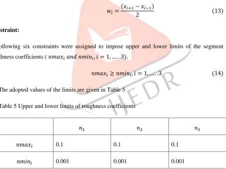
discretized by the discrete sections. Thus (𝑤_𝑖) is defined as follows:

𝑤𝑖 =

(𝑥_𝑖+1− 𝑥_𝑖−1)

2 (13)

Constraint:

i) Following six constraints were assigned to impose upper and lower limits of the segment

roughness coefficients ( 𝑛𝑚𝑎𝑥_𝑖 𝑎𝑛𝑑 𝑛𝑚𝑖𝑛_𝑖, 𝑖 = 1, … . .3).

𝑛𝑚𝑎𝑥_𝑖 ≥ 𝑛𝑚𝑖𝑛_𝑖, 𝑖 = 1, … . .3 (14)

The adopted values of the limits are given in Table 5

Table 5 Upper and lower limits of roughness coefficients

𝑛1 𝑛2 𝑛3

𝑛𝑚𝑎𝑥_𝑖 0.1 0.1 0.1

(16)

ii) Following three constraints were assigned to ensure realistic relative roughness of the three

roughness coefficients.

𝑛₁ ≥ 𝑛₂ ≥ 𝑛₃ (15)

iii) Following constraints was assigned to impose upper and limits of fitting parameters (∝).

2 ≥ ∝ ≥ 1 (16)

Since the reported value of ∝ 1.5, a range of 1 to 2 was prescribed.

Linked simulation optimization approach is used to estimate the optimal values of the parameters

for three bed conditions i.e d50=20mm, d50=6mm and lined concrete as bed materials and their

corresponding GVF profiles were simulated.

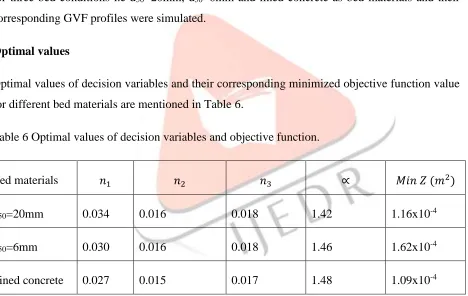
Optimal values

Optimal values of decision variables and their corresponding minimized objective function value

for different bed materials are mentioned in Table 6.

Table 6 Optimal values of decision variables and objective function.

Bed materials 𝑛₁ 𝑛₂ 𝑛₃ ∝ 𝑀𝑖𝑛 𝑍 (𝑚2)

d50=20mm 0.034 0.016 0.018 1.42 1.16x10-4

d50=6mm 0.030 0.016 0.018 1.46 1.62x10-4

Lined concrete 0.027 0.015 0.017 1.48 1.09x10-4

Optimal reproduction of GVF profiles

Computed GVF profiles corresponding to the optimal parameter values and the variation of

composite roughness are in the following figures. The profile is plotted for three different bed

(17)

Fig. 5 Observed reproduction of GVF profiles ( Q=8.601x10-3 m3/s and d50=20mm)

Fig. 6 Optimal reproduction of GVF profiles ( Q=8.601x10-3_m3_{/s and d}

50=20mm)

0.00 0.05 0.10 0.15 0.20 0.25 0.30 0.35 0.40

0 5 10 15 20 25

H1=0.25m H2=0.30m H3=0.35m

x (m) D

e p t h

(

m₎

0 0.05 0.1 0.15 0.2 0.25 0.3 0.35 0.4

0 5 10 15 20 25

H2=0.25m H2=0.30m H3=0.35m

x (m) D

e p t h

(

(18)

Fig. 7 Observed reproduction of GVF profiles ( Q=9.233x10-3 m3/s and d50=6mm )

Fig. 8 Optimal reproduction of GVF profiles ( Q=9.233x10-3_m3_{/s and d}

50=6mm)

0.00 0.05 0.10 0.15 0.20 0.25 0.30 0.35 0.40

0 5 10 15 20 25

H1=0.25m H2=0.30m H3=0.35m

x (m) D

e p t h

(

m₎

0 0.05 0.1 0.15 0.2 0.25 0.3 0.35 0.4

0 5 10 15 20 25

H2=0.25m H2=0.30m H3=0.35m

x (m) D

e p t h

(

(19)

Fig. 9 Observed reproduction of GVF profiles ( Q=9.314x10-3 m3/s and lined concrete)

Fig. 10 Optimal reproduction of GVF profiles ( Q=9.314x10-3_m3_{/s and lined concrete)}

Estimated parameters

The bed roughness (𝑛₁) varies from 0.027 to 0.034 as bed material /condition changes from lined

concrete to gravel (d50=20mm). The corresponding reported/ Strickler’s estimates are given in

0.00 0.05 0.10 0.15 0.20 0.25 0.30 0.35 0.40

0 5 10 15 20 25

H1=0.25m H2=0.30m H3=0.35m x (m) D e p t h ( m₎ 0 0.05 0.1 0.15 0.2 0.25 0.3 0.35 0.4

0 5 10 15 20 25

(20)

Table 5.2 by using equation 1.2. It may be seen that optimal roughness estimates are higher than

Strickler’s estimates.

Table 7 Reported/Strickler’s estimated optimal estimates for bed materials

Bed material/condition Reported/Strickler’s Estimation Optimal estimates

d50=20mm 0.0247 0.034

d50=6mm 0.0202 0.030

Lined concrete 0.013-0.015 0.027

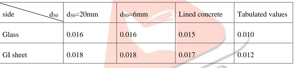
The roughness coefficient of glass and GI sheet sides as optimized for various runs are presented

in Table 8.

Table 8 Reported/Strickler’s estimates and optimal estimates for sides

side d50 d50=20mm d50=6mm Lined concrete Tabulated values

Glass 0.016 0.016 0.015 0.010

GI sheet 0.018 0.018 0.017 0.012

The estimated roughness coefficients satisfy the known inequality (𝑛₂ < 𝑛₃) and are higher than

the tabulated values. This establishes the credibility of the proposed model.

The optimal value of ∝ (fitting parameter) ranges from 1.42 to 1.48, which differs from the

reported value i.e. 1.5. The optimal value of ∝ increases as the bed materials get finer.

Reproduction of observed profile

Computed GVF profiles corresponding to the optimal parameter values match quite well with

corresponding observed profiles.

(21)

It can be observed that composite roughness reduces with increase in flow depth. Apparently

because of increase in weightage of side resistance, the value of composite roughness increase.

CONCLUSION

This study was carried out to identify open channel flow parameters. Manning’s roughness

coefficient and other parameters are estimated for different bed materials used ( d50 =20mm grain

size , 6mm grain size particles and Lined concrete bed materials). Also, based on the estimated

value of Manning roughness coefficient and flow depths, GVF flow profile is identified.

An optimization method is applied to identify the parameters based on Manning formula for

estimation of manning roughness coefficient and corresponding manning roughness parameters.

This estimation invokes the data of observed GVF profiles and such accounts for different bed

materials with the flow depth.

Experimental works is done to several sets of data monitored in Hydraulics Laboratory of Civil

Engineering Department. The application led to the following conclusions;

i) The GVF profile computed on the basis of estimated parameters match quite closely

with the corresponding observed profiles.

ii) Strickler’s formula under estimate the roughness due to the bed material.

iii) The following commonly used formula is calibrated for Manning coefficient

estimation

𝑛𝑐 =(∑ 𝑛𝑖

∝_𝑃 𝑖 𝑁

𝑖=1 )1/∝

(∑𝑁 𝑃_𝑖

𝑖=1 )1/∝

iv) The currently documented value of ∝ is 1.5. However, the present work reveals that it

varies from 1.42 to 1.48. The value of ∝ generally decreases as the bed material gets

coarser.

(22)

1. Atanov, G. A., Evseeva, E. G., and Meselhe, E. A. (1999). ‘‘Estimation of roughness

profile in trapezoidal open channel.’’ J. Hydraul. Eng., 125(3), 309–312

2. Ayvaz MT (2013). A linked simulation–optimization model for simultaneously

estimating the Manning’s surface roughness values and their parameter structures in

shallow water flows. Journal of Hydrology. 2013; 500: 183-199

3. Barros A.P and Calello J.D.,(2001), ‘’surface Roughness for shallow over land flow on

crushed stone surfaces’’, J.Hydraulics. Eng. ASCE. Vol. 127, No.1, January. Pp.38-52

4. Becker, L., and Yeh, W. W.-G. (1972). ‘‘Identification of parameters in unsteady open

channel flows.’’ Water Resour. Res., 8(4), 956–965.

5. Bennett, A. F., and McIntosh, P. C. (1982). ‘‘Open ocean modeling as an inverse

problem: Tidal theory.’’ J. Phys. Oceanogr., 12, 1004–1018.

6. Candela A, Noto LV, Aronica G. Influence of surface roughness in hydrological response

of semiarid catchments. Journal of Hydrology. 2005; 313(3-4): 119-131.

7. Chow, V.T., (1959), ‘’open channel Hydraulics’’, McGraw-Hill, New York

8. Christodoulou G.C., (2014), ‘’Equivalent Roughness of submerged obstacles in open

channel flow’’, J.Hydraulics. Eng. ASCE. Vol.140, No.2, February, pp.226-230

9. Das A., (2000), ‘’optimal channel cross section with composite roughness’’, J.Irrig.Drain.

Eng. ASCE. Vol.126, No.1, January, pp 68-72

10.Das, S. K., and Lardner, R. W. (1991). ‘‘On the estimation of parameters of hydraulic

models by assimilation of periodic tidal data.’’ J. Geophys. Res., [Oceans], 96, 15187–

15196

11.Dey S., (2000), ‘’Chebyschev solution as Aid in computing GVF by standard step

method’’, J.Irrig.Drain. Eng. ASCE. Vol.128, No.4, July/August, pp.271-274

12.Ding Y., Jia. Y. and Wang S.S.M., (2004), ‘’Identification of Manning’s Roughness

coefficient in shallow water flows’’, J.Hydraulics. Eng. ASCE. Vol.130, no.6, June,

pp.501-510

13.Esfandiari M. and Maheshwari B.L., (1998), ‘’suitability of selected flow Equations and

variation of Manning’s n in furrow Irrigation’’, J.Irrig.Drain. Eng. ASCE. Vol.124, No.2,

(23)

14.Guo Y., Zhang L., Shen Y., and Zhang J., (2008), ‘’Modeling study of free overfall in a

rectangular channel with strip Roughness’’, J .Hydraulics. Eng. ASCE. Vol.134, No.5,

May, pp. 664-667

15.Hameed L.K, and Ali T., (2013), Estimating of manning’s Roughness coefficient for

Hilla River through calibration using HEC-RAS Model’’, Jordan J. Civil Eng. Vol.7,

No.1, October, pp. 44-53

16.Hessel R., Jetten V., and Guanghi Z., (2003), ‘’Estimating Manning’s n for steep

slopes’’, CATINA, vol.54, No. 1-2, November. Pp. 77-91

17.Ishii, A. (2000). ‘‘Parameter identification of Manning roughness coefficient using

analysis of hydraulic jump with sediment transport.’’ Kawahara Group Research Report,

Chuo University, Japan

18.Jarret R.D., (1984), ‘’Hydraulics of High Gradient Streams’’, J .Hydraulics. Eng. ASCE.

Vol.110, No.11, November, pp.1519-1539

19.Koza JR. Human-competitive results produced by genetic programming. Genetic

Programming and Evolvable Machines. 2010; 11(3-4): 251-284.

20.Li Z. and Zhang J., (2001), ‘’calculation of field Manning’s Roughness Coefficient’’,

Agricultural water management, Vol.153, No.49, January 1, pp.152-161

21.Mailapalli D.R., Raghuwanshi N.S., Singh R., Schmitz G.H., and Lennartz F., (2002),

‘’spatial and temporal variation of Manning’s Roughness Coefficient in furrow Irrigation’’, J. Irrig.Drain. Eng. ASCE. Vol.134, No.2, April, pp.185-192

22.Naidu B.J, Bhallamudi S.M., Narasimhan S., (1997), ‘’GVF Computation in Tree-type

channel networks’’, J .Hydraulics. Eng. ASCE. Vol.123, No.8, August, pp.700-708

23.Navon, I. M. ~1998!. ‘‘Practical and theoretical aspect of adjoint parameter estimation

and identifiability in meteorology and oceanography.’’ Dyn. Atmos. Oceans, 27~1–4!,

55–79

24.Panchang, V. G., and O’Brien, J. J. (1989). ‘‘On the determination of hydraulic model

parameters using the strong constraint formulation.’’ Modeling marine systems, Vol. I, A.

M. Davies, ed., CRC Press, Boca Raton, Fla., 5–18.

25.Prevost, C., and Salmon, R. (1986). ‘‘A variational method for inverting hydrographic

(24)

26.Qin J. and Ng S.L., (2012), ‘’Estimation of effective roughness for water worked gravel

surfaces’’, J .Hydraulics. Eng. ASCE. Vol.138, No.11, November, pp.923-934

27.Ramesh R., Datta B., Bhallamudi S.M. and Narayana S., (2000), ‘’optimal estimation of

roughness in open channel flows’’, J .Hydraulics. Eng. ASCE. Vol.126, No.4, April, pp.

299-303

28.Reddy H.P., and Bhallamudi S.M., (2004), ‘’Gradual Varied Flow computation in cyclic

looped channel network’’, J. Irrig.Drain. Eng. ASCE. Vol.130, No.5, October, pp.

424-431

29.Rodríguez-Caballero E, Cantón Y, Chamizo S, et al. Effects of biological soil crusts on

surface roughness and implications for runoff and erosion. Geomorphology. 2012;

145-146: 81-89.

30.Stone B.M, and Hung T.S., (2002), ‘’Hydraulic Resistance of flow in channels with

cylindrical Roughness’’ J .Hydraulics. Eng. ASCE. Vol.128.,No.5, May, pp.50-506

31.Subramanya, K., (2012), ‘’flow in open channel’’, McGraw-Hill, third edition.

32.Urquhart, W. J. (1975). Hydraulics: Engineering field manual, U.S. Department of

Agriculture, Soil Conservation Service, Washington, D.C.

33.Vatankhah A.R., (2012), ‘’Direct Integration of Manning based GVF Equation in

trapezoidal channels’’, J. Hydrol. Eng. ASCE. Vol.128, No.3, March, pp. 445-462

34.Yeh, W. W.-G. (1986). ‘‘Review of parameter identification procedures in groundwater

hydrology: The inverse problem.’’ Water Resour. Res., 22(2), 95–108.

35.Zou, X., Navon, I. M., and Le Dimet, F. X. (1992). ‘‘An optimal nudging data

assimilation scheme using parameter estimation.’’ Q. J. R. Meteorol. Soc., 118, 1163–