A Generic Matrix Method to Model the Magnetics of Multi-Coil Air-Cored IPT Systems

A Generic Matrix Method to Model the Magnetics of

Multi-Coil Air-Cored IPT Systems

†

Prasanth Venugopal *†, Soumya Bandyopadhyay, Pavol Bauer and Jan Abraham Ferreira

Delft University of Technology (TU Delft), Mekelweg 04, 2628 CD, Delft, The Netherlands; [email protected] (S.B.); [email protected] (P.B.); [email protected] (J.A.F.) * Correspondence: [email protected]; Tel.: +31(0)15 2786016

† This paper is an extended publication of conference papers published by authors in [1]-[2]

Abstract: This paper deals with a generic methodology to evaluate the magnetic parameters of contactless power transfer systems. Neumann’s integral has been used to create a matrix method that can model the magnetics of single coils (circle, square, rectangle). The principle of superposition has been utilised to extend the theory to multi-coil geometries such as double circular, double rectangle and double rectangle quadrature assuming linearity of magnetics. Numerical and experimental validation has been performed to validate the analytical models developed. A rigorous application of the analysis has been carried out to study misalignment and hence the efficacy of various geometries to misalignment tolerance. Comparison of single-coil and multi-coil shapes considering coupling variation with misalignment, power transferred and maximum efficiency is carried out.

Keywords:air-cored; contactless; coupling; inductive power transfer; magnetics; matrix; modelling; multi-coil

1. Introduction

Inductive Power Transfer (IPT) relies on electromagnetic fields to transfer energy between circuits that are not physically connected. Loosely coupled coils that are used in IPT systems suffer from high leakage fields that demand reactive power, constricting large power transfer at high efficiency. To nullify this effect, capacitive compensation is carried out such that reactive power exchange take places between the capacitors and inductors with the source directly connected to the load, improving power factor, power transfer and efficiency.

Inductive Power Transfer systems due to its non-contact nature allows efficient power flow to happen with reduced maintenance, is safe, clean and reliable. Thus, applications spanning from low power medical devices (mW) to mining (MW) have been found in literature [3]. Other applications include consumer electronics, EVs, underwater power delivery etc [4], [5]. A number of resonant topologies have been proposed and several coil shapes and designs have been researched in this field [3]. However, an analytical framework that studies the impact of coil shape and misalignment in IPT systems in a rigorous manner is found missing.

The magnetic design and its optimization is an important step in the design of IPT systems. Typically, coil optimization and magnetic parameter estimation(L1,L2,M,k)are performed relying

on EM field solvers and/or combing with evolutionary algorithms [6,7]. In other work, numerical techniques (solving look-up tables (book of Grover [8]), solving Bessel functions [9], solving elliptical integrals [10] ) and PEEC solvers [11,12] are used to achieve the same. In Grover’s book, there is available closed-form expressions for self-inductance of a number of polygonal shapes. However, all the equations are developed for single-turns ignoring the effect of the air-gap between turns resulting in a reduction in a reduced fill factor.

In this paper, we bridge this gap by taking into account the effect of turns (increase in perimeter for every new turn) as well as any incipient air-gap by using a matrix manipulation. This extends to both single and multi coil geometries and their magnetic behaviour is analysed.

2. Neumann’s Integral

The mutual inductance between two current carrying circuits assuming uniform cross-sectional current density and neglecting radiation can be written in terms of the differential length vector of the two circuitsdl1~ ,dl2~ separated by a distancer12as

L12=

λ2 i1 =

µ0

4π I

c1

I

c2 ~

dl1.dl~2

r12 (1)

In equation1, contoursc1andc2are along the middle edge of the circuits 1 and 2 (primary and secondary) respectively. This equation is generic, order independent and can be adapted to model self-inductance by considering the contoursc1andc2as along the middle edge of the conductor and the inner edge of the wire.

2.1. Circular Coils

In case of a pair of circular coils, the application of Neumann’s integral as in (1), the two contours

c1 and c2 represent the contour of current filaments assumed to be in the middle of primary and

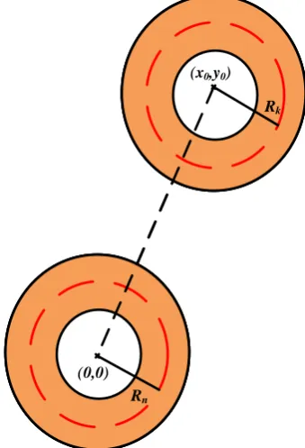
secondary. Now, consider the case of a misaligned circular coil pair, composed of wires of circular cross-section of radius r and with an air-gaplgbetween turns. Such a coil pair is indicated in Figure 1. The inner radius of theithturn of the primary andjthturn of secondary areRi=Rp+ (i−1)(2r+

Rn

Rk

(0,0)

(x0,y0)

Rn

Rk

(0,0)

(x0,y0)

Figure 1. A coupled circular coil system with primary havingi = 1, 2...,nturns and the secondary havingj=1, 2...,kturns, the radii of the mid current contour of thenthprimary turn andkthsecondary turn areRnandRk.

lg),Rj =Rs+ (j−1)(2r+lg)respectively. In such a case, the partial mutual inductance is written in terms of azimuths,φiandφjof the respective coils as

Mij=

µ0

4π × "

Z 2_π

φi=0

Z 2_π

φj=0

Idφidφj #

WhereI,Ri,Rjare defined as

I = q RiRjsinφisinφj+RiRjcosφicosφj

Ricosφi−(x0+Rjcosφj)2+ Risinφi−(y0+Rjsinφj)2

(3)

The final mutual inductance can be defined for primary having0n0turns and secondary with0k0

turns as

M= n

∑

k

∑

Mij (4)

The self-inductances can be extracted similarly from (4) by defining the radius of the middle edge and the inner edge of each turn.

2.2. Rectangular Coils

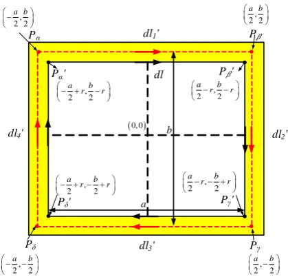
A single turn rectangular coil is shown in Figure2. A rectangular structure can be split into four sections (l₁0,l

20, ..l40), each of which refer to conductors in the top, bottom, left and right respectively

In such a case, (1) can be written in terms of the various sections of the coil as

Pα P

Pδ Pγ

, 2 2 a b

_ 

 

 

 0, 0

a b

, 2 2 a b

 

 

 

,

2 2

a b

 _ 

 

 

,

2 2

a b

_{ } 

 

 

,

2 2

a b

r r

_{  } 

 

  2 ,2

a b

r r

 _{ } 

 

 

,

2 2

a b

r r

 _{  } 

 

 

,

2 2

a b

r r

_{   } 

 

 

Pα' P '

Pγ'

Pδ'

dl1'

dl2'

dl3'

dl4'

dl

Figure 2.Definition of the contour of the elementary inner edge of a single turn rectangular coildland the various sections of the contour of the elementary line along the centre of the wire(dl₁0,dl

20, ..dl40).

For further evaluation, the contour ofdlcan be split at the top, right, bottom and left sections as

(dl1,dl2, ..dl4).

L= µ0 4π×

" I

l

10

I

l1

d−l→₁0.d

−→

l1 r₁0

1 +

I

l

20

I

l1

d−→l₂0.d

−→

l1 r₂0

1 +

I

l

30

I

l1

d−l→₃0.d

− →

l1 r₃0

1 +

I

l

40

I

l1

d−l→₄0.d

−→

l1 r₄0

1

#

(5)

which the inductance contribution is considered. Each element of the matrix is a partial inductance (self partial inductance(i=j)and mutual partial inductance(i6=j)).

Lij =

µ0

4π×                   H l 10 H l1

d−l→

10.d − →

l1 r

101

H l

10

H l2

d−l→

10.d −→

l2 r

102

· · · H

l

10

H l4

d−l→

10.d −→

l4 r

104

H l

20

H l₁

d−l→

20.d − →

l1 r

201

H l

20

H l2

d−l→

20.d −→

l2 r

202

· · · H

l

20

H l₄

d−l→

20.d −→

l4 r

204

H l

30

H l₁

d−l→

30.d − →

l1 r

301

H l

30

H l2

d−l→

30.d −→

l2 r

302

· · · H

l

30

H l₄

d−l→

30.d −→

l4 r

304

H l

40

H l₁

d−l→

40.d − →

l1 r

401

H l

40

H l2

d−l→

40.d −→

l2 r

402

· · · H

l

40

H l₄

d−l→

40.d −→

l4 r

404

                  (6)

Self-inductance of this rectangular coil can be written as

L= 4

∑

∑

Lij (7)

Since the orthogonal terms in the vector dot product reduces to a zero. For eg: (dl~₁0.dl2~ = dx1iˆ.dyjˆ=0).

L=     

L11 0 L13 0

0 L22 0 L24

L31 0 L33 0

0 L42 0 L44

     (8)

Thus, the total external self-inductance can be written in terms ofLa = L11 = L33,Lb = L22 = L44,Ma=L13=L31,Mb =L24 =L42as

L=2(La+Lb−Ma−Mb) (9)

Where, the self-partial inductances(La,Lb =L(a=b))are given by

La= µ0 4π×

" Z a

2−r −a 2+r dx1 Z a 2 −a 2 dx2 p

(x2−x1)2+r2

#

La= (a−r)ln

a−r+pr2_{+ (a−r)}2

−a+r+pr2_{+ (−a+r)}2

+rln

−r+√2r

r+√2r

+2√2r−

q

(r2_{+ (a−r)}2₎₋q_(r2_{+ (−a+r)}2₎

(10)

Also, the mutual partial inductances(Ma,Mb= M(a↔b))are given as

Ma=

µ0

4π × "

Z a

2−r −a 2+r dx3 Z a 2 −a 2 dx2 p

(x2−x3)2+ (b−r)2

#

(11)

3. Multi-Turn Charge Pads

of turns. It is useful to list the vertices of the extremes of the contour along the center of the wire as well as along the inner edge of the wire for theNthwinding.

2r

lg

(0,0) _b

a

Pα P

Pδ Pγ

2r

lg

(0,0) _b

a

Pα P

Pδ Pγ

Top section (1)

Left section (4) Right section (2)

Bottom section (3)

1,2,3..Nturns

Figure 3. A multi turn inductor with dimensions defined from the centre of a wire of circular section with radius r and wound in a manner such that air gap is uniform (lg)

and the center contour of the wire has vertices Pα = (−a/2,b/2), Pβ = (a/2,b/2),

Pγ = (a/2,−b/2), Pδ = (−a/2,−b/2). The Nth turn ‘α

0 _{vertex has its middle edge}

and inner edge with vertices PNα =

h −a

2−(N−1)(2r+lg),b2+ (N−1)(2r+lg)

i

and PNαi =

h

−a₂+r

−(N−1)(2r+lg),

b

2−r

+ (N−1)(2r+lg)

i .

The partial self-inductance of theNthturn (due to the 1stsection) can be derived as

LN1N1=

µ0

4π × "

Z k₂

k1

dx1

Z _β

α

dx2

p

(x2−x1)2+r2

#

(12)

Where,

k1=−a

2+r

−(N−1)(2r+lg),k2=

a 2−r

+ (N−1)(2r+lg)

α=−a

2−(N−1)(2r+lg),β=

a

2+ (N−1)(2r+lg)

(13)

The result of such an integration is

µ0

4π×[I(C=β)−I(C=α)] (14)

Where,

I(C) = q

r2_{+ (C−k} 2)2−

q

r2_{+ (C−k} 1)2+ln

q

r2_{+ (C−k}

1)2+ (C−k1)

(C−k1)

q

r2_{+ (C−k2)}2_{+ (C−k2)}

(C−k2)

(15)

Lijlk =

µ0

4π ×                N

∑

∑

Li1l1 0 −

N

∑

∑

Li1l3 0

0 N

∑

∑

Li2l2 0 −

N

∑

∑

Li2l4

− N

∑

∑

Li3l1 0

N

∑

∑

Li3l3 0

0 − N

∑

∑

Li4l2 0

N

∑

∑

Li4l4

               (16)

The diagonal terms in the above matrix are the sectional partial self-inductance and the off-diagonal terms are the sectional partial mutual inductance. Note that the signs of sectional self-inductance are positive and sectional partial mutual inductance are negative for rectangular structures. The summation terms can be evaluated by calculating some general matrices like

LN1k1,LN1k3. The inductance contributions of LN2k2,LN2k4 can be obtained by inverting a ↔ b in

the previous set of general expressions. The net self-inductance can then be written as

L= N

∑

∑

∑

∑

Lijlk (17)

3.1. Sectional Partial Inductances

The sectional partial self-inductance is defined as the sum of the partial self and partial mutual inductance contributions of current in a particular section on the same section on all possible turns. The sectional partial mutual self-inductance is defined as the sum of the partial mutual inductance contributions of current in a particular section on a different section for all combinations of possible turns. Following the previous procedures, the partial self-inductance due to current in theNthturn first section on thekth_{turn first section is given by}

LN1k1=

µ0

4π× 

 Z k₂

k1 dx1 Z _β α dx2 q

(x2−x1)2_{+ r+ (N−k)(2r+l} g)2





Symbols:

k1=−a

2+r

−(k−1)(2r+lg),k2=

a 2−r

+ (k−1)(2r+lg)

α=−a

2 −(N−1)(2r+lg),β=

a

2+ (N−1)(2r+lg)

(18)

The result of this integration is the same as (14) withI(C)defined as

I(C) = q

(r+ (N−k)(2r+lg))2+ (C−k2)2

−

q

(r+ (N−k)(2r+lg))2+ (C−k1)2

+ln q

(r+ (N−k)(2r+lg))2+ (C−k1)2+ (C−k1) (C−k1)

q

(r+ (N−k)(2r+lg))2+ (C−k2)2+ (C−k2) (C−k2)

(19)

LN1k3=

µ0

4π× 

 Z k₂

k1 dx1 Z β α dx2 q

(x2−x1)2+ (b−r) + (2r+lg)(N+k−2)2 



Symbols:

k1=

−a

2+r

−(k−1)(2r+lg),k2=

a 2−r

+ (k−1)(2r+lg)

α=−a

2−(N−1)(2r+lg),β=

a

2+ (N−1)(2r+lg)

(20)

Again, the result of this integration is the same as (14) withI(C)defined as

I(C) = q

((N+k−2)(2r+lg) + (b−r))2+ (C−k2)2

−

q

((N+k−2)(2r+lg) + (b−r))2+ (C−k1)2

+ln q

((N+k−2)(2r+lg) + (b−r))2+ (C−k1)2+ (C−k1) (C−k1)

q

((N+k−2)(2r+lg) + (b−r))2+ (C−k2)2+ (C−k2)

(C−k2)

(21)

4. Mutual Inductance between rectangular coils

Pα _P

Pδ Pγ

Pα _P

Pδ Pγ

a b dl1'

dl2'

dl3'

dl4'

0,0,0

     

Pα P

Pδ Pγ

Pα P

Pδ Pγ

dl1 dl2 dl3 h d c

Pα P

Pδ Pγ

dl1 dl2 dl3 h d c r rs , 2 2 a b      

  2 2,

a b         , 2 2 a b          , 2 2 a b          0,0,h            cd,h

2 ,

2 

   cd_,h

2 , 2      cd,h

2 ,

2 

   cd_,h

2 , 2       c d,h

2 , 2      _c_d_,h

2 ,

2 _ c d,h_

2 , 2      _c_d_,h

2 , 2

Pα _P

Pδ Pγ

a b dl1'

dl2'

dl3'

dl4'

0,0,0

     

Pα P

Pδ Pγ

dl1 dl2 dl3 h d c r rs , 2 2 a b      

  2 2,

a b         , 2 2 a b          , 2 2 a b          0,0,h            cd,h

2 ,

2 

   cd_,h

2 , 2       c d,h

2 , 2      _c_d_,h

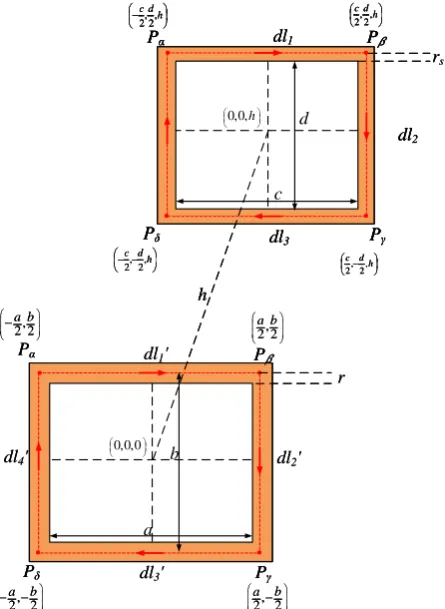
2 , 2

A simple description of the mutual inductance scenario of a single turn primary and a single turn secondary is depicted in Figure4. As an extension of the theory previously developed, the mutual inductance for a multi-turn rectangular coil can be written in terms of the contributions due to current flowing throughithturn, jthsection of the primary on thelthturn,kthsection on the secondary. The sectional mutual inductance matrix can be written as

Mijlk =

µ0

4π×                N

∑

∑

Mi1l1 0 −

N

∑

∑

Mi1l3 0

0 N

∑

∑

Mi2l2 0 −

N

∑

∑

Mi2l4

− N

∑

∑

Mi3l1 0

N

∑

∑

Mi3l3 0

0 − N

∑

∑

Mi4l2 0

N

∑

∑

Mi4l4

               (22)

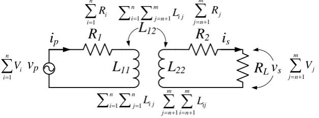
5. Extension to MCCP

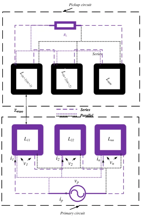
Consider a linear magnetic system excited by a pure sinusoidal (non-harmonic) voltage consisting of a primary and pickup composed of several segmented coils as shown in Figure5. The coils can be individually connected serially or in parallel to compose the multi-coil charge-pad. Let the primary be composed of0n0coils,(1, 2, ..n)and pickup with0m−n0coils,(n+1,n+2, ..m,(m>n)). Consequently, the voltage matrix,hVifor all the coils can be written as a in terms of currents,hiiand time-derivative of currents,h_dtdii

h

Vi=hLi×hdi dt i

+hRi×hii (23)

Where the matrices are defined as

[V] =                 v1 v2 .. . vn vn+1 vn+2

.. . vm                 di dt = i0 =                

i0₁ i0₂

.. .

i0n i0_n+1 i0_n+2

.. .

i0_m

               

[i] =                 i1 i2 .. . in in+1 in+2

.. . im                

[R] =      

R1 0 0 0 0 0 0 0

0 R2 0 0 0 0 0 0

..

. ... ... ... ... ... ... ...

0 0 0 0 0 0 0 R8

v1

v1 vv22 vvnn

vn+2

vn+2

vn+1

vn+1 vvmm

vs

vs

vp

ip

ip

i2

i2 iinn

in+1

in+1 iin+2n+2 iimm

is

is

v1 v2 vn

vn+2

vn+1 vm

vs

vp

ip

i2 in

in+1 in+2 im

is

v1 v2 vn

vn+2

vn+1 vm

vs

vp

ip

i2 in

in+1 in+2 im

is

i1

i1

L11 L22 Lnn

L11 L22 Lnn

L11 L22 Lnn

L11 L22 Lnn

RL

RL

L11 L22 Lnn

RL

Zairgap Series

Parallel Series Parallel

L11 L22 Lnn

RL

Zairgap Series

Parallel

v1 v2 vn

vn+2

vn+1 vm

vs

vp

ip

i2 in

in+1 in+2 im

is

i1

L11 L22 Lnn

RL

Zairgap Series

Parallel Series Pickup circuit

Primary circuit

Figure 5. Defining a IPT system with primary and secondary composed of multiple coils with self-inductances as(Lij,i=j)and mutual inductances as(Lij,i6=j).

Finally,[L]is defined as

[L] = 

              

L11 L12 . . . L1n L1(n+1)L1(n+2). . . L1(m) L21 L22 . . . L2n L2(n+1)L2(n+2). . . L2(m)

..

. ... ... ... ... ... ... ...

Ln1 Ln2 . . . Lnn Ln(n+1)Ln(n+2). . . Ln(m) L(n+1)1L(n+1)2. . . L(n+1)n 0 0 0 0 L(n+2)1L(n+2)2. . . L(n+2)n 0 0 0 0

..

. ... ... ... 0 0 0 0

Lm1 Lm2 . . . Lmn 0 0 0 0



              

(25)



   

n

∑

vi m

∑

vj 

   

= 

   

n

∑

n

∑

Lij n

∑

m

∑

Lij m

∑

n

∑

Lij m

∑

m

∑

Lij 

   

×

"

ip0 is0 #

+ 

    n

∑

Ri 0

0

m

∑

Rj 

   

×

"

ip is #

(26)

The Equation (26) indicates that it is possible to convert a linear magnetic system with multi-coil

L

L

R

L

R

R

v

i

i

v

j j n

V

 



1 n

i i

V





1 m

j j n

R

 



1 n

i i

R





1 1

n n

i j

i j

L

 

1 1

n m

i j i j n 

L

 

1 1

m m

ij

j n i n

L

   

 

Figure 6.Equivalent single coil pair for a system of coils with(1, 2..n)coils in the primary and(n+

1,n+2..m)coils in the pickup.

into a system of a single coil pair by calculating the individual contributions. Such a equivalent coil system is shown in Figure6. Such a transposition makes it easy to analytically model multi-coil linear magnetic systems by using the principles of single coils already developed previously.

6. Validation of Analytical Model

To validate the analytical models that are developed in previous sections, FEM simulation and experimentation are carried out. Circular and rectangular shapes are compared. The physical properties of the coils are tabulated in Table 1. To show the efficacy of analytical expressions, a reduced fill factor was employed for rectangular coils by maintaining an air-gap of 0.6 cm between the turns.

Table 1.Properties of the compared circular and rectangular coils

Type of coil a(cm) b(cm) lg(cm) N (turns)

Rectangular(R1) 4 2 0.6 9

Rectangular(R2) 6 4 0.6 15

Circular(C) inner diameter = 5.5 cm 14

litzwire used 600×0.071 mm, 2.1 mm dia overall

The constructed coils are shown in Figure7. The measurements, analysis and simulations are carried out at variable z-gaps between the coils and also at several misaligned positions. The z-gaps are simulated at 3, 5, 7 and 9 cms of coil displacements in the z-direction, taking vertical misalignment in consideration. In case of lateral misalignment, perfect alignment, 75%, 50% and 25% alignments are chosen along x-axis. The results along y-axis for symmetrical shapes follows the same trend as the x-axis and hence are not considered.

Figure 7.Experimental comparison of rectangular and circular coils with parameters as tabulated in Table1.

by connecting the coils serially from one end to the other and then swapping one of the ends (Lconst, Ldes). The expressions used for extracting the mutual inductance and coupling are

M= Lconst−Ldes 4

k= √M

L1L2

(27)

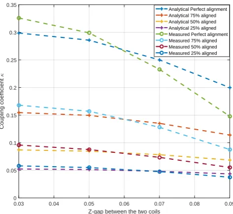
The analytical expressions for circular coils are calculated from Equations (1) −(4). Also, for rectangular coils, Equations (12)− (22) are computed. MATLAB scripts are written separately for each of the computation and a software tool for self, mutual and coupling computations is developed for air-cored coils. A comparison of coupling obtained analytically and by making measurements for circular coils is presented in Figure8.

0.03 0.04 0.05 0.06 0.07 0.08 0.09

Z-gap between the two coils 0

0.05 0.1 0.15 0.2 0.25 0.3 0.35

Coupling coefficient

5

Analytical Perfect alignment Analytical 75% aligned Analytical 50% aligned Analytical 25% aligned Measured Perfect alignment Measured 75% aligned Measured 50% aligned Measured 25% aligned

The results show a large degree of agreement between the analytical expressions and the measured results. Mismatch in the results are due to the use of litz wire in the experiments (unlike a solid conductor used in the analysis) and eddy currents (proximity effects) in the coils that are not considered in the analytical expressions. Some instrumental accuracy limitations also add to this error. However, most observations are within 1% accuracy except for an odd set in the neighbourhood of 6%. These accuracy measures are acceptable for magnetic analysis.

FEM models were created and simulated so as to perform numerical evaluation of the coils considered. The FEM models developed are presented in Figure9.

Figure 9. FEM simulation models of the rectangular coil (top-left), circular coil (top-right) and the rectangular coil (bottom) couple. The rectangular coils are modelled in a 3d domain while the circular coils due to their rotational symmetry are modelled in the 2d domain.

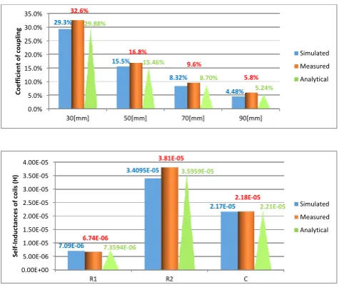
The coupling and self-inductances of circular and rectangular coils are compared analytically, using FEM simulations and experimentation. The results are presented in Figure10, the coupling being recorded at perfect alignment and variable z-gaps while self-inductances measured for all variable shapes. All measurements show the same trend and there is a close match between analytical observations, FEM simulations and measurements.

0.0% 5.0% 10.0% 15.0% 20.0% 25.0% 30.0% 35.0%

30[mm] 50[mm] 70[mm] 90[mm]

29.3%

15.5%

8.32%

4.48%

32.6%

16.8%

9.6%

5.8% 29.88%

15.46%

8.70%

5.24%

Co

e

ff

ic

ie

n

t

o

f c

o

u

p

lin

g

Simulated

Measured

Analytical

0.00E+00 5.00E-06 1.00E-05 1.50E-05 2.00E-05 2.50E-05 3.00E-05 3.50E-05 4.00E-05

R1 R2 C

7.09E-06

3.4095E-05

2.17E-05

6.74E-06

3.81E-05

2.18E-05

7.3594E-06

3.5959E-05

2.21E-05

Se

lf

-In

d

u

ctan

ce

s o

f c

o

ils

(H

)

Simulated

Measured Analytical

7. Shape and Performance of Air Couplers

The effect of shapes in IPT systems can be analysed for air-cored couplers based on the mathematical analysis that has been derived previously. To make such a comparison, a few performance parameters are considered. They are the open circuit voltagevoc, short circuit currentisc, maximum output power,smax and maximum efficiency,ηmax. Open circuit voltage is the maximum voltage that the IPT system can source and short circuit current is the maximum current that the same can deliver.

For a coupled charge-pad, ifL1andL2are the self-inductances of the two couplers with ‘M0as the mutual inductance and operated at angular frequencyω, creating currenti1through the primary,

the open-circuit voltage is defined asvoc= jωMi1and during short-circuit ifiscis the current flowing in the pickup,isc = voc

jωL2 =

Mi1

L2 . Now, the maximum output power is defined in terms of loaded

quality factor of pickup,Q2L = (ω×L2)/(RL+R2), whereRL is the load resistance andR2is the

ac-resistance of the pickup charge-pad as

smax=voc×isc= (i2

1M2Q(2,L)ω) L2

(28)

The above equation quantifies the maximum output power that such an air-cored coupler can source. Also, the maximum efficiency of IPT systems have been derived independent of compensation applied and load present in terms of native quality factors of the primary(Q1) and pickup(Q2)as [13]

ηmax = k

√

Q1Q2

2+k√Q1Q2 (29)

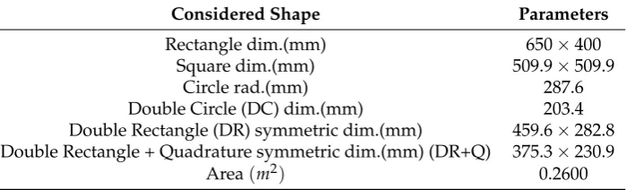
These parameters have been used to compare a number of differently shaped air-cored charge-pads. All shapes considered have been analysed keeping area conserved. This way, generalizations of the behaviour of fields and hence coupling, power transferred and other parameters are possible. Several analysis were also carried out keeping perimeter conserved and multi-turns with similar results. In addition, these results also correspond and can be generalized to charge-pads with flux-enhancing materials such as ferrite. This as enhanced coupling is obtained by placing ferrites along the natural direction of flux lines. Hence, the basic tendency of the shape in terms of coupling and its gradient is similar in all IPT applications. The compared shapes are listed in Table2. All considered shapes have been simulated with a one turn coil and a z-gap of 1 cm. This so that the effect of shapes are more enhanced.

Table 2.Physical parameters of various coil shapes used in the air-cored coupler.

Considered Shape Parameters

Rectangle dim.(mm) 650×400

Square dim.(mm) 509.9×509.9

Circle rad.(mm) 287.6

Double Circle (DC) dim.(mm) 203.4

Double Rectangle (DR) symmetric dim.(mm) 459.6×282.8 Double Rectangle + Quadrature symmetric dim.(mm) (DR+Q) 375.3×230.9

Area(m2) 0.2600

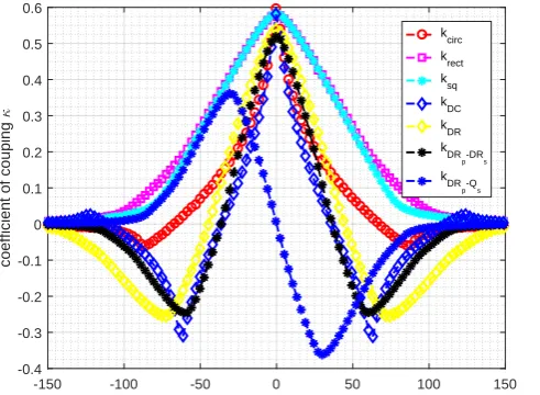
A study of coupling by misaligning the coils along x-direction (lateral displacement) is presented in Figure11.

-150 -100 -50 0 50 100 150

% coupling along X-direction represented as a percent of rectangle edge a = 650mm

-0.4 -0.3 -0.2 -0.1 0 0.1 0.2 0.3 0.4 0.5 0.6

coefficient of couping

5

k

circ

k

rect

k_sq k_DC k

DR

k_DR

p-DRs

k

DR

p-Qs

Figure 11. Coupling coefficients of single and multi-coil shapes with x-directional misalignment of coils in Table2.

It can be inferred that circle and four sided shapes differ in the tolerance to coupling variations when subjected to lateral misalignment. The coupling of rectangular and square coils tend to decay gradually, while the circular shape sees a more sharper drop with misalignment. Circular shape due to the fact that it has the highest area for a given perimeter among closed shapes, has the highest coupling at the best aligned point. The double coils also share the same feature but with a larger extension of the power profile. It is important to note that in this analysis, since area is kept conserved, the perimeter varies between the shapes and hence it is important to keep trends in mind, rather than absolute values. Null-coupling points in DR and DC coils, occur at positions where a pick-up coil is confronted with opposing flux of equal magnitude from the primary charge-pad. Among the double coils, the DC geometry has greater best-aligned coupling than that of DR geometry. However, the misalignment profile for DR coils is broader than that of DC coils and hence it is well suited to applications where larger misalignment behaviour is expected, for eg: EVs. When such an analysis was broadened to include the behaviour of a DR primary and a DRQ pick-up, the Q picking up flux emanating from a DR primary behaves best at the misaligned points, while is the worst at the best-aligned point. On the contrary, the DR pick-up behaves complementary to the Q pick-up with a DR primary.

-150 -100 -50 0 50 100 150

% Misalignment along X-direction with edge of the rectangle a = 650mm

0 0.1 0.2 0.3 0.4 0.5 0.6

Uncompensated power s

max

in p.u.

Circular Rectangular Square DC DR DR_p-(DR+Q)_s

Figure 12. Uncompensated power analysed on the basis of a unit current flowing through various shapes of single turn and equal area as indicated in Table2. The misalignment is considered along x-direction.

The maximum efficiency as presented in Equation (29) has dependence on quality factor which in-turn depend on the ac resistances of the coils. The ac-resistances for thelitzwire used is extracted from a tabulation technique as presented in [14]. The calculated ac resistance factor including both skin and proximity effects for litz wire indicated in Table1is Rac

Rdc

= 1.029. The result of maximum

efficiency computation when subjected to variable coupling during misalignment is shown in Figure

13. This plot represents the theoretical maximum efficiency that can be expected at various misaligned points for various shapes. The efficiency values floor at the power null points as expected.

-150 -100 -50 0 50 100 150

% Misalignment along X-direction with edge of the rectangle a = 650mm

0 0.1 0.2 0.3 0.4 0.5 0.6 0.7 0.8 0.9 1

Maximum efficiency profile for tracking

2 max

Circular Rectangular Square DC DR DR_p-DR_s DR

p-Qs

Figure 13.Maximum efficiency profile tracking with x-directional misalignment of coils in Table2.

8. Discussion

be present in charge-pads is the next step. Such a FEM optimisation for a 1kW DR system is presented in [15]. Some useful results obtained from the analysis are:

1. The analysis, compared with FEM and experiments have a good match. Almost all observations have an error less than 10%. This is acceptable for magnetic analysis.

2. The coupling of single coils are such that circular coils have the best coupling at the well-aligned point and the four shaped coils have a larger misalignment tolerant band. Thus, rectangular coils can be used for more misalignment tolerant designs and circular for well-aligned applications.

3. The coupling behaviour of multi-coil geometries follow the trend of single-coil shapes but have null-coupling points. By designing a Q coil located between the mid points of the single-coils, flux can be captured at the null-coupling points.

4. The Q and DR pickup have complementary coupling-misalignment behaviour. At the best aligned point, the Q picks up no flux and at the misalignment point of null-coupling of DD pickup, the Q picks up maximum flux.

5. The DR and DC shapes can effectively extend the range of power transfer to larger misaligned positions. The addition of Q to the pickup can remove null-coupling points from the power profile.

6. Rectangular coils also perform well with the same enclosed area as multi-coil geometries, with a lesser zone of power transfer.

7. The total enclosed area of the shapes has been kept constant to make a fair comparison. However, it is possible to influence the turns in the Q coils in DRQ and this impacts the peaks obtained in the misalignment points. For designing IPT systems that are adapted to misalignment as in EVs during motion, dynamic power transfer, a DR charge pad on the roadway would be a good solution optimizing the excess material costs involved in building DRQ pads. Also, EVs travelling along the regions of power null for a long time is limited. However, for stationary charging, misalignment tolerant DRQ charge pad for both primary and secondary is a good choice for good power transfer. Also, interoperability is possible between these pads thus making it possible to have the same vehicle pads for both modes of operation.

Author Contributions: “V.P. is the primary investigator. S.B. made several numerical models to evaluate the theory developed. P.B. and J.A.F. are the supervisors who directed the study and gave valuable suggestions and shared their experiences in this field.”

Conflicts of Interest:“The authors declare no conflict of interest.”

References

1. Prasanth, V.; Bauer, P.; Ferreira, J.A. A sectional matrix method for IPT coil shape optimization. In International Conference on Power Electronics and ECCE Asia (ICPE-ECCE Asia), Daejeon, Korea, 5–6 June 2015, pp. 1684–1691.

2. Prasanth, V.; Bandyopadhyay, S.; Bauer, P.; Ferreira, J.A. Analysis and comparison of multi-coil inductive power transfer systems. In Power Electronics and Motion Control Conference (PEMC), 2016 IEEE International , Varna, Bulgaria, 25–30 Sept 2016, pp. 993–999.

3. Covic, G.A.; Boys, J.T. Modern Trends in Inductive Power Transfer for Transportation Applications. IEEE

Trans. Emerg. Sel. Topics Power Electron.2013,1, 28–41.

4. Prasanth, V.; Bauer, P. Distributed IPT Systems for Dynamic Powering: Misalignment Analysis.IEEE Trans.

Ind. Electron.2014,61, 6013–6021.

5. Shekhar, A.; Prasanth, V.; Bauer, P; Bolech, M. Economic Viability Study of an On-Road Wireless Charging System with a Generic Driving Range Estimation Method.Energies2016,9, 76.

6. Budhia, M.; Covic, G.A.; Boys, J.T. Design and optimization of circular magnetic structures for lumped inductive power transfer systems.IEEE Trans. Power Electron.2011,26, 3096–3108.

8. Grover, F.W.; InInductance Calculations: Working Formulas and Tables; Dover Publications, 1946.

9. Convway, J.T. Inductance calculations for noncoaxial coils using bessel functions. IEEE Trans. Mag. 2007,

43, 1023–1034.

10. Maxwell, J.C.; InA Treatise on Electricity and Magnetism; Cambridge University Press: Cambridge, UK, 2010. 11. Ruehli, A.; Paul, C.; Garrett, J. In Proceedings of International Symposium on Electromagnetic

Compatibility, 1995 pp. 7–12.

12. Musing, A.; Ekman, J.; Kolar, J.W. Efficient calculation of non-orthogonal partial elements for the peec method.IEEE Trans. Mag.2009,45, 1140–1143.

13. Takanashi, H.; Sato, Y.; Kaneko, Y.; Abe, S; Yasuda, T. A large airgap 3kw wireless power transfer system for electric vehicles. In Energy Conversion Congress and Exposition (ECCE) , 2012 IEEE, pp. 269–274. 14. Terman, F.E.; InRadio Engineer’s Handbook; 1943.