Improving the learning of self-driving vehicles
based on real driving behavior using Deep Neural
Network Techniques
Nayere Zaghari1 , Mahmood Fathy2, Seyed Mahdi Jameii3, Mohammad Sabokrou4, Mohammad Shahverdy5
1Department of Computer Engineering, Shahr-e-Qods Branch, Islamic Azad University, Tehran, Iran
2 School of Computer Science, Institute for Research in Fundamental Sciences Tehran, Iran
3 Department of Computer Engineering, Shahr-e-Qods Branch, Islamic Azad University, Tehran, Iran
4 School of Computer Science, Institute for Research in Fundamental Sciences (IPM)
5 Department of Computer Engineering, IRAN University of Science and Technology (IUST), Tehran, IRAN
Corresponding Author: Mahmood Fathy, [email protected]
Abstract Considering the significant advancements in autonomous vehicle technology, research in this field is of interest to researchers. To drive vehicles autonomously, controlling steer angle, gas hatch, and brakes need to be learned. The behavioral cloning method is used to imitate humans’ driving behavior. We created a dataset of driving in different routes and conditions and using the designed model, the output used for controlling the vehicle is obtained. In this paper, the Learning of Self-driving Vehicles Based on Real Driving Behavior Using Deep Neural Network Techniques (LSV-DNN) is proposed. We designed a convolutional network which uses the real driving data obtained through the vehicle’s camera and computer. The response of the driver is during driving is recorded in different situations and by converting the real driver’s driving video to images and transferring the data to an excel file, obstacle detection is carried out with the best accuracy and speed using the Yolo algorithm version 3. This way, the network learns the response of the driver to obstacles in different locations and the network is trained with the Yolo algorithm version 3 and the output of obstacle detection. Then, it outputs the steer angle and amount of brake, gas, and vehicle acceleration. The LSV-DNN is evaluated here via extensive simulations carried out in Python and TensorFlow environment. We evaluated the network error using the loss function. By comparing other methods which were conducted on the simulator’s data, we obtained good performance results for the designed network on the data from KITTI benchmark, the data collected using a private vehicle, and the data we collected.
Keywords: Autonomous vehicle,Self-driving, Real Driving Behavior, Deep Neural Network, LSV-DNN.
1
Introduction
Research and development in the field of machine learning and more precisely deep learning lead to many discoveries and practical applications in different domains. The domain where machine learning has a huge impact is the automotive industry and the development of fully autonomous vehicles.
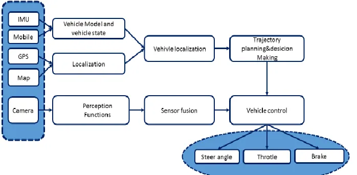
Machine learning solutions are used in several autonomous vehicle subsystems, as the perception, sensor fusion, simultaneous localization and mapping, and path planning. In parallel with work on full autonomy of commercial vehicles, the development of various automotive platforms is the current trend. For example, delivery vehicles or various different robots and robot-vehicles are used in warehouses [1]. The autonomous driving system can be generally divided into four blocks: sensors, perception subsystem, planning subsystem, and control of the vehicle, Figure 1.
Figure 1: Autonomous vehicle system block diagram [1].
The main idea of our work was to develop a solution for autonomous driving for a light automotive platform that has limited hardware resources, processor power, and memory size. Having those hardware restrictions in mind, we are aiming to design a light deep neural network (DNN), an end-to-end neural network that will be able to perform the task of autonomous driving on the representative track, while the developed networks’ model used for inference is possible to deploy on the low-performance hardware platform. This paper comprises two main phases: Phase one is the detection of obstacles around the vehicle. We considered the detection of different moving and stationary obstacles including pedestrians, benches, parked vehicles, overtaking vehicles, etc., and sometimes we do not have any obstacles and want to detect the roads and turning left and right while moving.
In phase two, real driving methods are applied to autonomous vehicles according to the processing carried out in phase one which include obstacle and motorway detection in order to improve the learning in autonomous vehicles. Then, the network is trained and generates steer angle, acceleration, and brake as output.
The paper presented here is organized as the following. Section 2 presents the related works. In Sect. 3 brings the proposed LSV-DNN framework.Moreover, results and discussion of the implementation of LSV-DNN and inference during autonomous driving are given in section 4.Finally, in Section 5, the paper is concluded.
2
Related works
In this section, we review existing work on the learning of self-driving vehicles as well as work on visual explanation and justification.
network. The core gradient of deep neural networks are convolutional networks. Convolutional neural networks (CNN) are a specialized kind of neural network for processing data that has a known grid-like topology. CNNs combine three architectural ideas: local representative fields, shared weights, and spatial or temporal sub-sampling, which leads to some degree of shift, scale, and distortion invariance. Convolutional neural networks are designed to process data with multiple arrays (e.g., color image, language, audio spectrogram, and video), and benefit from the properties of such signals: local connections, shared weights, pooling, and the use of many layers. For that reason, CNNs are most commonly applied to analyzing visual imagery [4, 5].
The first successful attempts of the development of autonomous vehicles started in the 1950s. The first fully autonomous vehicles were developed in 1984 [6,7], and in 1987 [8]. Significant breakthrough in the field of autonomous vehicles is done during the Defense Advanced Research Projects Agency’s (DARPA) challenge, Grand Challenge events in 2004 and 2005 [9,10], and Urban Challenge in 2007 [11], where it was demonstrated that machines could independently perform the complex human task of driving.
However, application on real-time embedded platforms with limited computational power and, memory spaces seeks for a different approach [12]. Since the execution of DNN depends heavily on the weights, also called model parameters, the solution for deep neural network architecture suitable for applications on embedded platforms is the smaller model that needs to communicate less data. This is challenging to achieve, especially if the application is computer vision and that has, as an input, a high-quality image. The reduction of the neural network depth and number of parameters often leads to accuracy degradation. Hence, by developing deep neural networks for computer vision for embedded platforms we are looking for a solution that will be good enough for both an acceptable accuracy and the possibility for inference on hardware platforms with limited capabilities. Therefore, our goal is to develop the right deep neural network architecture that can achieve acceptable accuracy, the successful autonomous driving in a representative track, but which operates in real-time within power and energy limitations of its target embedded automotive platform.
An additional motivation for the use of end-to-end systems can be found in related problems [13]. An end-to-end neural network based on camera images to fly a drone through a room. They stress that using pre-trained networks is a good alternative to learning from scratch for end-to-end networks. It saves training time and requires less data because it is less prone to overfitting. They also stress that training LSTM networks using a limited time window produces better performance than when training it on all previous input samples. Moreover, [13] indicates that there is a clear trend in which LSTM networks outperform standard feedforward networks. [14] also used LSTMs combined with other techniques to tackle end-to-end driving. Another observation is that recovery cases have a big impact on performance. Following the same directions, [15] demonstrates that it is possible for networks trained on simulation data to be generalized to the real world. Taking these works into account, it is plausible to assume that many observations and conclusions drawn from the autonomous drone problem, such as the generalization of simulators and the better performance of LSTM networks, also hold for our problem. Finally, motivation for incorporating inter-frame dependencies is found in language modeling. Just like different words in a sentence are also related in order to convey meaning, the input images are temporally dependent because they are consecutive frames of a video. It is proven that LSTMs can outperform standard feedforward neural networks on such tasks [16, 17].
Based on similar ideas, modern self-driving vehicles [19, 20] have recently started to employ a batch IL approach: with DNN control policies, these systems require only expert demonstrations during the training phase and on-board measurements during the testing phase. For example, Nvidia’s PilotNet [20], a convolutional neural network that outputs steering angle given an image, was trained to mimic human drivers’ reactions to visual input with demonstrations collected in real-world road tests.
CNN is a type of feed-forward neural network computing system that can be used to learn from input data. Learning is accomplished by determining a set of weights or filter values that allow the network to model the behavior according to the training data. The desired output and the output generated by CNN initialized with random weights will be different. This difference (generated error) is back propagated through the layers of CNN to adjust the weights of the neurons, which in turn reduces the error and allows us produce output closer to the desired one [21].
A notable approach [22] addressing the problem of understanding classification decisions by pixel-wise decomposition of non-linear classifiers proposes a methodology called layer pixel-wise relevance propagation, where the prediction is back propagated without using gradients such that the relevance of each neuron is redistributed to its predecessors through a particular message-passing scheme relying on the conservation principle. The stability of the method and the sensitivity to different settings of the conservation parameters was studied in the context of several deep learning models [23].
TheLayer-wise Relevance Propagation (LRP) technique was extended to Fisher Vector classifiers [24] and also used to explain predictions of CNNs in NLP applications [25]. An extensive comparison of LRP with other techniques, like the deconvolution method and the sensitivity-based approach, which we also discuss next in this section, using an evaluation based on region perturbation. This study reveals that LRP provides better explanation of the CNN classification decisions than considered competitors.
3
The proposed LSV-DNN framework
In the following section, we design the learning of self-driving vehicles schema by employing deep neural network techniques. The proposed system consists of three Phases; such as an overview of the LSV-DNN model is discussed in Phase 1. The detection of obstacles around the vehicle is discussed in Phase 2. The next section's real driving methods are applied to autonomous vehicles is discussed in Phase 3.
3.1Phase 1: Overview of the LSV-DNN model
gradually). Therefore, acceleration type or measuring acceleration are some of the most important criteria for the driver’s behavior whether it is while the vehicle is moving straight, turning left, or overtaking another vehicle. The distance to the vehicle in front is another important one of driver’s behavior criteria. Also, the driver should maintain the distance limit to obstacle or vehicles on the road when obstacles are seen. In an aggressive driving, the autonomous vehicle might move closer and farther from the vehicle in front. This kind of driving is hazardous and causes problems for the passengers of this vehicle and the passengers of other vehicles. While in real and pleasant driving, the vehicle adjusts its distance and speed using the speed limit of the road such that it is not hazardous and observes the matter of perception and reaction time in terms of traffic.We describe the problem in seven steps as Fig. 2.
Figure 2: General seven steps of the study
Figure 3 shows the autonomous driving system in this research.
Figure 3: The autonomous driving system in this research
3.2Phase 2: Detection of obstacles around the vehicle
Step one: gathering data
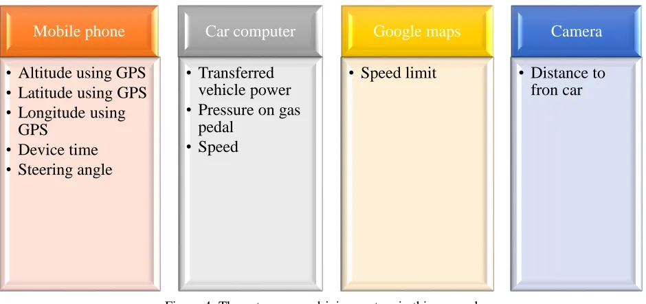
In step one, we have provided logistics for installing cameras on the vehicle, using the IMU of the vehicle computer while driving absolutely safely, and recording vehicle and camera data during the safe drive we had on the highway. In this step, we have first gathered the data. The intended vehicle was equipped with data gathering devices so that it can save the data required for detecting driver’s behavior according to the proposed architecture. To do this, a device was installed for communicating with the vehicle computer which transfers speed, RPM, amount of pressure on the gas pedal, and vehicle defects wirelessly to the computer or mobile phone. Also, a mobile phone was installed on the steering wheel for measuring acceleration, steering wheel rotation angle, the geographical location of the vehicle, and road tilt. To measure the distance to the front vehicle, a camera was used which records video from front vehicles with a 30 frame per second accuracy. Distance to the front vehicle is determined by detecting its license plate and measuring its area with a below 40-centimeter error. Measuring distance is carried out using radar in advanced vehicles. However, because we did not have access to this technology, we used image processing instead. The data regarding the surrounding environment including traffic levels, road windings, speed limit, and road type was obtained from google maps.
Step two: data pre-processing
This step includes creating the excel file containing the data gathered while driving, including rotation angle while driving safely, brake, gas, condition, and location of the vehicle obtained from vehicle’s computer system, and converting the video to image frames. In this step, pre-processing and image normalization was carried out. Also, the values obtained from the aforementioned equipped vehicle in different traffic and road conditions were tested and data was collected with a 100-millisecond frequency. Fields of initial harvested data without preprocessing is presented in the Figure 4.
Figure 4: The autonomous driving system in this research
Normal driving contains the driver’s normal behavior including safe and allowed speed, avoiding too accelerating or decelerating speed, paying attention to the road, observing the distance to vehicles in front and on the side, driving between the lanes, etc. The driver being examined in this test must observe these items. We will gather the collected dataset in a CSV1 file and use as input for the
1 Comma Separated Values
Mobile phone
• Altitude using GPS • Latitude using GPS • Longitude using
GPS
• Device time • Steering angle
Car computer
• Transferred vehicle power • Pressure on gas
pedal • Speed
Google maps
• Speed limit
Camera
designed network and study the results afterward. To this end, a file comprising acceleration measurements, steering wheel turning angle, the geographical location of the vehicle, road tilt on the wheel, distance to the front vehicle, speed data, RPM, pressure on the gas pedal, and vehicle problems columns.
Then, we saved the recorded videos as frames and matched each frame to the information we have in the Excel file. After collecting data and loading data into the network, we need data processing steps. In the next step, we preprocess the data. This data along with the images taken using the camera, which were saved as frames, are the network input. At this step, we analyze the data and preprocess useless parts of the images like obstacles in the lane facing the vehicle or obstacles on the roadside which are considered to be noise. One data distribution method is distribution histogram. Histogram graph is a variable which abides by the normal distribution and its normality has been proven. In fact, if after drawing the graph we observe that histogram shape is symmetrical and a bell-like shape, its normality can be accepted. In this project, we need catalogs which are as follows. A file containing the images and reports which will be used for training the model which we save under the name ‘model’ in the clone. After collecting data, it is essential we know what distribution they follow.
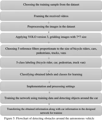
Step three: obstacle detection
Figure 5: Flowchart of detecting obstacles around the autonomous vehicle
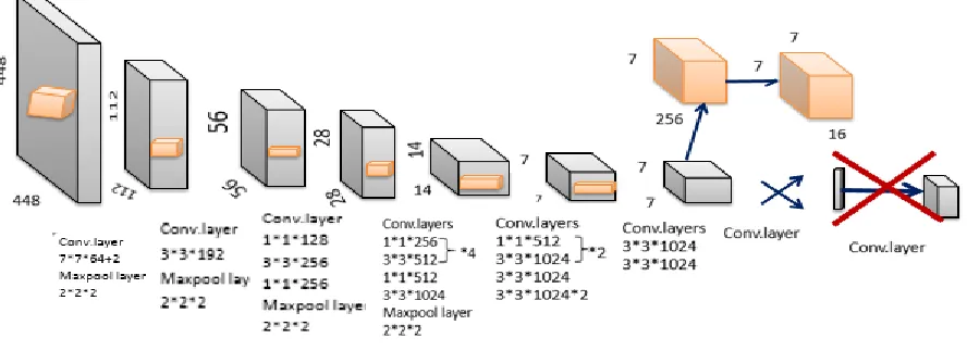
We carry out obstacle detection on the images extracted from the video recorded while driving using the YOLOv3 algorithm. In the classification method, image content is identified and we assign a label to the image. However, the location and class name must be reported for each sample of an object in obstacle detection. Also, there is no limit on the number of objects in an image and usually the location of each object is specified using a bounding box (bbox). Therefore, we need an algorithm that can do these things at a high speed. The YOLOv3 algorithm extracts features and classifies the objects in the image using convolutional layers. In this algorithm, multiple objects are detected in the images. In other algorithms, a sliding window is convolved with the image and a part of the image the size of the sliding window is fed to convolutional layers each time. Each time, we have an output vector and at the next step, the window moves and these steps are repeated on the next part of the image. In the end, we have a fully-connected layer. In the YOLO algorithm, these steps are carried out simultaneously using multiple windows and it searches for gridded images with multiple sliding windows. when multiple sliding windows carry out feature extraction simultaneously, we get multiple output vectors at the same time which improves the speed. In this algorithm, fully-connected layers are removed from the end of the layers and feature extraction is done using several extraction boxes. This helps speed up the process.The YOLOv3 is given in Fig. 6.
Choosing the training sample from the dataset
Framing the received videos
Preprocessing the images in the dataset
Applying YOLO version 3, gridding images with 7*7 size
Implementation and processing settings
Training the network using training data and detecting objects around the car Choosing 5 reference filters proportionate to the size of bicycle riders, cars,
pedestrians, trucks, vans
5-class labeling (bicycle rider, car, pedestrian, truck van)
Classifying obtained labels and classes for learning
Figure 6: YOLOv3
In the YOLOv3, the authors present a novel and deeper architecture for feature extraction called Darknet-53. As it is clear from its name, it contains 53 annular layers. Each layer is followed by a batch normalization layer and Leaky ReLU activation function. Sampling is done from below using dense layers with stride = 2. The second version of YOLO was called YOLO9000. The detection algorithm uses a proposed regional network to detect objects in input images and a single tracker SSD Multi-box Detector. The next version is YOLO version 3. The accuracy and speed advantages of YOLO version 3 have led to its superiority. In this version, a specific score will be predicted for each box using logistic regression. Multi-class classification is possible in the classifier. For instance, we will have the probability of each class between being human and man. YOLO version 3 extracts features using Darknet-53 which is deeper than Darknet-19 uses by the second version of YOLO.The Darknet-53 is given in Fig. 7.
Figure 7: Darknet-53
Figure 8: Overall structure of the YOLO system along with the input and the output
Each boundary box has 5 elements (x, y, w, h, confidence score). X and Y are the coordinates of the object in the input image. W and H represent the width and height of the object respectively. Confidence score is the probability of the box having an object and its accuracy.The boxes border is given in Fig. 9.
Figure 9: Boxes border
The YOLO algorithm is based on regression where object detection, positioning, and classification for an input image is carried out with a single action. These algorithms are usually used for object detection in real-time. The disadvantage of YOLO version one is that it does not detect small objects. The YOLO architecture is given in Fig. 10.
Figure 10: Boxes, input, and output of the YOLO architecture
Score, abjectness score, or confidence means how probable it is for the bounding box (bbox) to contain an object.
x, y: specifies the upper right point in each bbox
width: specifies the width of the bbox
height: specifies the height of the bbox
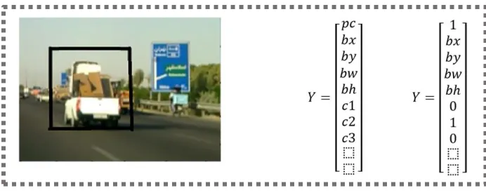
In object detection, we specify the location of the objects and classify them. When there is more than one object in an image, we find the location of each object using a bounding box. This can be carried out using a simple convolutional network. This network carries out classification and 4 numbers are specified for the bounding box location. The coordinates, including X and Y, along with w and h, representing width and height, are the output. This means that in addition to the bounding box, it specifies their position as well. We have the ground truth for training the box. We compare the predicted box to the ground truth and square their difference and obtain the sum of squared errors function. By minimizing this function, better answers can be found which means better boxes can be chosen and the object positions can better be detected. So, in addition to the classification we always received, we have the properties of the bounding box as well. Therefore, we solve a specific classification problem along with a regression problem at the same time. Assume we have multiple objects like vehicles, pedestrians, and bicycle riders. We have three classes for three objects. We consider a fourth class as the background as well. While generating the training set, when we select parts of the images on random for this algorithm, the objects often are not in that part. This means there is no object in the part we selected and the fourth class belongs to these backgrounds which do not contain any objects. this way, we create the training set. The bounding box can be specified through many methods. For example, using the center point along with length and width or a chosen point along with the length and the width, etc. We also create an output vector for each input image. Output vectors of the bounding box from the image is given in Fig. 11.
Figure 11: Output vectors of the bounding box from the image
This vector contains one column and 8 rows for 3 classes. The first row is pc which is the probability of an object being in the image and is either zero or one. For example, if there is an object in the image, the value of pc will be set to one and if there are no objects, pc will be set to zero. The next rows are the coordinates of the object in the bounding box. Parameters bx, by, bw, and bh correspond to the x and y (coordinates) and h and w (height and width). While c1, c2, and c3 are the defined object classes like vehicle, pedestrian, and bicycle. The corresponding class parameters get set to one for whichever class is found in the bounding box. After the detection of the object, we evaluate the error using the loss function. The loss function can be used to minimize these numbers and carry out the object detection task. The output can be zero and one at the same time. However, if an object is not present, this does not happen, meaning that it doesn’t matter what value other rows have in case pc = 0 and we do not need to use them in the sum of squared errors function.
which can be used to detect multiple objects is Sliding Window. In this technique, we crop different parts of the image while creating the training set and determine whether there were any objects in any part of the image. Since the size of the objects is not determined, we use different windows to crop the image. Therefore, it is not cost-effective at all to use the sliding window technique because we would need to convolve the image with different windows over and over again and obtain the value from their multiplication. The idea is to give the image as the system input only once and identify all the objects in the image and receive them in the output. The idea for object detection is that we implement a convolutional network in a fully convolutional form, meaning that we do not have fully connected layers at the end and we also use convolutional layers instead of fully connected ones. To this end, the YOLO algorithm grids the images for object detection as well and checks different part of the image concurrently using several anchor boxes. This way, sliding window calculations are simultaneous and we get an output vector for each window. Each part of the grid we have considered for an image corresponds to a part of the image and the output of each part is available for object presence probability and classification.
While detecting an object, we have the ground truth which is the real box and a predicted bounding box. We calculating the amount of overlap between these two boxes, which is the similarity and overlap between two boxes corresponding to the presence of an object. The overlapping value is a number between 0 and 1 calculated using similarity distance (the IOU criterion). Assume for example that we want to detect the object in the image. We have 2 bounding boxes which if they are similar (we calculate the similarity between the two bounding boxes using the IOU criterion), we can detect the object. If the object is labeled as 1 in the output, this object is a vehicle or if it gets a value of 0, it means that the object is not a vehicle. If the overlapping between these two boxes is more than a threshold, it means that the object is detected. For calculating this criterion, we only need to measure their area and divide the area of their intersection to the area of their union.
Steps of the YOLOv3 algorithm:
1. We use a grid to divide the image into multiple parts
2. We represent training data like figure 14.3. Assuming C to be the number of unique data points in our
dataset, S S* will be the number of networks to which we divide our images. Our output vector will have
a length of S S* *(C+5). In the above case, for example, our target vector is 4*4*(C+5)because we
have divided our images to a 4*4 grid and we train for 3 unique objects, i.e. vehicle, light, and pedestrian.
3. We create a deep annular neural network with the dropout operation as an error between outputs of activations functions and the generated label vector. In fact, the output model predicts the outputs of all
networks with a single pass of the input image using.ConvNet
4. The label of the object in a grid is determined if the object is present in it. An object is not labeled several times in different networks.
we have labels for each network cell where an anchor boxes are needed. If an object is assigned to an anchor box in the grid, another object can be assigned to another anchor box in the same grid.
With the YOLOv3 algorithm, detecting the obstacles around the vehicle is done in minimum time and with the highest accuracy on the KITTI dataset. The goal of image processing is to track each frame in the video and separate the background from target objects after removing the random noise from the images. The current methods include optical flow, background subtraction [51], frame difference methodsetc. These methods have simple steps and high detection speed. However, these methods still have some flaws. The background subtraction method needs to obtain background images in advance and is sensitive to environmental factors like changes in lighting. This makes it susceptible to wrong judgment. The frame difference method is used for creating a difference between two or several consecutive frames in a video. If the environmental variation is small between these two frames, the frame difference method can obtain the moving object with accuracy. However, an object with a low movement speed might not be detected and environmental changes, like changes in lighting, might affect the results significantly. In this research, a combination of frame difference and background difference methods are used for background separation. A video is approximately 25 frames per second. Therefore, the delay between two consecutive frames is very short. Shifting background and object pixels change significantly. Therefore, we can assume that the luminance of a specific pixel follows the Gaussian distribution presented below.Gaussian distribution is given in Eq. (1).
(
)
(
)
1
0 1
, ,
N i
x y F x y
N
= −
(
)
1(
) (
)
0 1
, , ,
N i
x y F x y x y
N
= − −
(1)
Where
( )
x y, represents the coordinates of a pixel.It is worth noting that N (σ2, μ), B (x, y) is satisfied if μ represents the average difference of the Gaussian distribution and σ2 is the variance of the Gaussian distribution.
The Gaussian model is trained using the data pixel points and these two parameters are optimized during the progression of training. The difference operation on pixel point in the background of the image and grids of the previous image is carried out for obtaining different values. If this value is higher than the threshold value, it becomes evident that an object has been detected. The frame difference method is used for detecting moving regions. Changeable regions can be identified by comparing the difference between adaptor boxes and the threshold value. We use the frame difference method to eliminate the similarity between two frames and then adopt the background detection method for object detection. The Gaussian model is used for placing pixel points.Gaussian model is given in Eq. (2).
DK x y
(
,)
=
K x y(
,)
−
K−1(
x y,)
We carry out the obstacle detection steps in this problem using the YOLOv3 algorithm in autonomous vehicles on the KITTI dataset. In the received images, some parts of the image are not needed and we need to select features which affect driving. Some parts of the image do not present any correct information, like the vehicles on the opposite lane on the highway which need to be removed from the image. Also, to this end, we need obstacle detection steps with a standard evaluation criterion. The technique used for object detection in this research is YOLOv3. It is the most comprehensive real-time system in deep learning and solving image detection problems. First, this algorithm divides the image to different parts and marks each part. Then, it runs the detection algorithm in parallel on all of these sections to see which part belongs to which category. After the full recognition of objects, it connects them together so that every two main objects are in one box. All of these steps are run in parallel. Therefore, it is real-time and can process up to 40 images in one second. Although this model has a slightly worse performance compared to RCNN, it can be used for solving everyday problems because it is real-time. The YOLO architecture has brought some changes to object detection systems and looks at the object detection problem as a regression problem which gets directly from image pixels to box coordinates and class probabilities. Using the YOLO system, for detecting the objects in the image, you only look once. YOLOv3 has the DARKNET-53 network. Using these 53 layers, the model is more than strong enough even for the smallest objects in the image. YOLOv3 is able to detect more than 80 different objects in one image. YOLOv3 can reduce error significantly. YOLOv3 uses a bounding box with a thin size.
In this research, we will study processing on CUDA using TensorFlow and Keras frameworks. A graphics card with support for compute capability 3.5 or above (version 1.11.0 and above) is needed to be able to install the GPU version of TensorFlow and carry out processing on CUDA. We use the conda install tensorflow-gpu command for installation so that all the dependencies like cuda, cudnn, etc., are installed automatically. From version 1.8 onwards, CUDA8 and cuDNN6 are the oldest supported version of CUDA and cudnn which are supported (CUDA7.5 and cudnn5.1 and below are not supported from this version onwards and version 1.7 of TensorFlow is the last version which supports CUDA7.5 and cudnn5.1). With RTX series of NVIDIA vehicles (like RTX2060, RTX2070, etc.) one could install TensorRT so that we can enjoy a significant increase in speed using CUDA. To use the TensorFlow library of Python, we need to meet some requirements which will differ based on the type of CPU or GPU we are using. For the GPU version, only NVIDIA graphics cards which are compatible with CUDA are usable. The prerequisite of the CPU version of TensorFlow is Python but in the GPU version, the graphics card drivers, Cuda, and Cudnn must be installed on the system first. The process of processing with CUDA and TensorFlow is so that the data is copied from the main CPU memory to GPU memory. CPU sends processing instructions to the GPU. GPU cores carry out the instructions in parallel. The result is copied from GPU memory to the main memory.
Sum of squared errors function:
The YOLO algorithm divides images to a S*S grid and the output of each network has a (B*5+C) size and includes location, the confidence level of the bounding box, and the probability of the defined class information. The sum of squared errors function comprises three types of error.
(
)
2
0 S i
Loss=S
= coordErr+iouErr+classErr(3)
There are objects with different sizes in the image. We evaluate all boxes with any size using one criterion. We know the error is not the same in big boxes as it is in small boxes. In other words, an error pixel in a big box must be punished less than an error pixel in a small box. Using √, we punish big boxes less than we punish smaller ones. It suffices to compare y=x and y=√x charts. coordErr
represents the sum of squared position errors and is defined as follows:
(
) (
)
(
)
(
)
2 2 ^ ^ 1 2 2 ^ 1 ^ B objij i i
i
B obj
ij i
j
coordErr i x x y y
i W W h h
= = = − + − + − + −
(4)When iijobjis equal to one, it means that there is an object at the center of the I’th grid. Otherwise, its
value is zero. Value of IOU represents the amount of intersection between the current active bounding box with all reference bounding boxes. We choose the object with the maximum IOU value as the object detected by the current bounding box. iouError represents the number of squared errors of confidence level and is defined as follows:
iouErr=
Bj=1iijobj (
ci −c^)
2+
Bj=1iijnobj(
ci−c^)
2
(5)
ClassError represents the sum of squared error of classes and is defined as follows:
It is clear that these factors have different effects on object detection accuracy. Furthermore, many networks do not store objects and the confidence level of their created bounding boxes are zero which will lead to unstable training and divergence. Therefore, we define different weights for different networks. Usingcoord, we define different weights for image grids which represents the center of an object and where coord=0.5, represents the weights of grids where there is no object. Therefore, the improved loss function is as follows:
(
)
2
0 * *
s i
Loss=S
= coord coordErr+noobji iouErr+classErr(6)
3.3Phase 3: Applying realistic driving patterns for vehicles
are able to extract features automatically during training and eventually carry out the road segmentation and obstacle detection automatically with high accuracy.
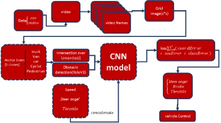
A convolutional neural network makes it possible to use the behavior of a vehicle during driving to obtain its location and speed and train the network. This network uses the information provided by front cameras, vehicle location on the road, and its speed. Driving data is obtained directly from real driving in the form of a video and the system learns to automatically drive on a striped road. This network automatically learns the internal representations of necessary processing, different functions are used and it realizes that the Exponential Linear Unit (ELU) function leads to improved learning compared to other activation functions. A behavioral simulation is a software where the behavior of a driver and his capabilities are transferred to the computer. To this end, the actions taken by the driver such as braking, pressing the gas, and changing the angle of the steer are recorded on the computer. This way, this behavior is transferred to the computer and finally, these actions are fed to the designed network as the driver’s behavior. In the next part, the system learns to output the parameters needed for driving according to the convolutional network we will design, the layers, defined weights, and activation functions we will consider. To this end, we have designed this research in multiple steps.The flowchart of proposed LSV-DNN is given in Fig. 13.
Figure 13: Flowchart of the LSV-DNNproposed model
The third phase consists of two steps.
Step one: designing the convolutional network
Convolutional networks contain several layers where we have a number of neurons. Each neuron receives a number of inputs and calculates the product of the multiplication of weights in the inputs. Finally, it presents a result using a non-linear transfer (activation) function. the network is a differentiable scoring function where the raw image pixels are on its one side and the scores corresponding to each set are on the other side. This type of networks has a loss function like Softmax or SVM at their last fully-connected layer. The input of the convolutional network are the images and we encode specific features in the architecture. By doing so, the forward function can be implemented more efficiently and also network parameter values decrease significantly. Neural networks get an input in the form of a vector and pass it through a number of hidden layers. Finally, an output, which is the result of the processing done in hidden layers, appears at the network output. Each hidden layer comprises a number of neurons and these neurons are connected to all the neurons in the previous layer. Neurons at each layer operate independently and are not related to each other at all. The last fully connected layer is known as the output layer and usually plays the role of presenting the score of each class. Normal neural networks are not scalable for full images. Therefore, a fully connected neuron in the first hidden layer of a normal neural network will have a weight of 32x32=3072. This value might not at first seem like a significant value but it is obvious that this fully-connected architecture will not be usable for larger images. For instance, an image with a more conventional size like 200x200x3 makes a neuron get a weight of 200x200x3=120,000. Furthermore, we will definitely want more neurons. Therefore, the number of parameters increases rapidly. It is clear that this full connectivity is wasteful and the large number of parameters will quickly lead to overfitting.
Each layer in the ConvNet organizes its neurons in 3 dimensions (width, height, and depth). Each layer of a ConvNet network transforms the input in the form of a dimensional mass to a three-dimensional output of neuron activation values. The ConvNet network comprises several layers and each layer have a simple way of working where it receives a three-dimensional mass input and uses differentiable functions, which might have parameters or have no parameters, to transform them to a three-dimensional output mass. Since the values of these step parameters are tuned automatically, we call it learning because the neural network is able to perform the detection task assigned to it by learning these parameters. Each layer of the convolutional network transforms an activation mass into another activation mass using a differentiable function. We use three main types of layers for creating a convolutional network architecture. These layers are as follows: Convolutional layer, Pooling layer, and fully-connected layer which is exactly like the ones we see in ordinary neural networks. We stack these layers on top of each other to create a complete convolutional network architecture.
We have designed an architecture with input, convolutional, RELU, POOL, and FC layers. The input layer contains out raw input pixel values. This means that we will have an image with a width of 32, height of 32, and 3 red, green, and blue channels. The Convolutional layer: this layer calculates the output of neurons which are connected to local regions in the input. The calculation operation is done through the scalar product of the weight of each neuron and the region it is connected to (input activation mass). The result of this operation is a mass of size 32x32x12.
The Pooling layer carries out the down sampling operation along spatial dimensions (width and height) which leads to a mass of size 16x16x12. In the pooling layer, we reduce the input mass (image) dimensions. In principle, it is through the operation of this layer that we obtain a score vector at the end of the convolutional network. The FC or fully-connected layer is responsible for calculating class scores. The result is a mass of size 1x1x10 where each one of 10 numbers represent the score of a specific class. Like ordinary neural networks and as can be inferred from the name of this layer, each layer in this network is connected to every neuron in the mass before it. With this method, the convolutional network transforms raw pixels of the original image to class scores at the end of the network layer by layer. Some layers have some parameters and others do not. Specifically, Conv/FC layers are the layers that apply transformations which not only are a function of activations (available values) in the input layer but also are a function of parameters like weight and bias of the neurons. On the other hand, RELU/POOL layers only implement a fixed function. The parameters present in Conv/FC layers are trained using the gradient descent method so that the class scores calculated by the convolutional network fit (are consistent with) the label of each image in the training set.
We train the weight of our network so that the sum of squared errors between the steering command output by the network and the human command or the steering command tuned for off-center images is turned. The following figure presents the network architecture which comprises 9 layers. A normalization layer, 5 convolutional layers, and 3 fully-connected layers of among them. Convolutional network architecture is given in Fig. 14.
Figure 14: Convolutional network architecture
has a distance less than the allowed limit, brakes will be used. Also, the opposite lane is removed from the image so that the vehicles on the opposite adjacent line are dismissed and only the vehicles in the same line are considered. The designed convolutional network comprises 5 convolutional layers, three fully-connected layers, and a normalization layer. The network uses GPU for fast processing and is implemented in the TensorFlow framework. In the first layer, image normalization is carried out. The convolutional layers are designed for feature extraction with respect to the research conducted in this field.
Step two: tuning the parameters
The network settings for learning, loading data to the network, and training the network designed for learning driver’s behavior and feature extraction like the optimization method, learning rage, momentum, and test iterations are specified. Learning tasks are divided between the solver and the network such that tasks like monitoring optimization and updating parameters are assigned to the solver and calculating the error and gradient values are assigned to the network. Organizing optimization, creating the training network, and creating testing networks are done to evaluate the network. Optimization is done by the solver by calling forward and backward repeatedly and updating network parameters, evaluating (periodically) the network, taking snapshots from the network model and solver condition. At each repetition of optimization, the forward phase is called to calculate the output and network error. Then, the backward phase of the network is called to calculate the gradients. Gradients are applied during parameter updating with respect to the method specified in the solver. The condition of the solver is updated according to learning rate, history, and the specified method so that we can transform the weights from the initial values to the learned model. There are various methods for optimization. The optimization methods specified in the solver address general optimization problems for reducing error.
4
Evaluating the Performance
Step one: evaluating obstacle detection and evaluating the error in the designed network
The dataset containing vehicle information which includes vehicle status, acceleration, brake, and steering wheel rotation angle and the video of vehicle surroundings from driver’s behavior during driving. The video is converted to image frames and vehicle information was procured in an excel file. First, We carried out obstacle detection using the YOLOv3 algorithm on image frames. Then,We divided the results along with the vehicle information found in the excel file input dataset to training and validation datasets with an 85/15 ratio and trained the designed CNN model. The goal of this project is predicting steering wheel angle and amount of gas and brake. We carry out obstacle detection using the IOU overlapping criterion and obtain the error rate using the sum of loss which was described in the previous section. We used the Adam optimizer to obtain the best Mean of Squared Errors (MSE) value for the predicted steering wheel angle. We used 10 rounds for training with a batch size of 64.
convolutional network will be trained using the data collected during the driving We have done. The network output which is the steering wheel rotation angle, acceleration, gas, and brake which has been carried out with little output time and a loss=0.650 network error. In the second project, obstacle detection in the designed convolutional network was carried out using three Resnet, Unet, and YOLOv3 algorithms on the KITTI data. The best results were obtained by YOLOv3 algorithm with IOU=0.98. To this end, I designed the proposed model with the YOLOv3 algorithm which presents better results. In this model, YOLOv3 algorithm detects the obstacles around the vehicle with five truck, vehicle, pedestrian, van, cyclist, and tram classes. This algorithm detects the objects around the vehicle using the standard KITTI data quickly and with high accuracy and presents the results to the designed convolutional network so that the network can be trained. This way, we can have the steering wheel angle, acceleration, gas, and brakes with high speed and accuracy.
In the next project, We carried out my second project on the data We had collected. First, obstacle detection was carried out with the YOLO algorithm on the data collected during driving with IOU=0.98 and network error is low according to the following results. We got very good results and the network has presented the steering wheel angle, gas acceleration, and brake after training.
Step two: routing and controlling the vehicle movement
In the last step, we give the outputs of the designed network which are the steering wheel rotation angle, gas acceleration, and brakes to the control system of the autonomous vehicle so that the vehicle can respond to the surrounding obstacles according to the responses it has learned and gas acceleration, brake, and the rotation angle are applied.Obstacle detection on the KITTI data using the Unet algorithm is given in Fig. 15.
Figure 15: Obstacle detection on the KITTI data using the Unet algorithm
Figure 16: Obstacle detection on the KITTI data using the Resnet algorithm
Figure 17: Obstacle detection has also been done using the YOLOv3 algorithm on the images obtained from real driving
Figure 18: Obstacle detection on the collected data using the YOLOv3 algorithm
In this research, we divided the input dataset to training and test sets with an 85/15 ratio and trained the CNN network. The goal of these projects is to predict steering wheel angle and this can be achieved using linear regression. To obtain the best mean squared error (MSE) value for the predicted steering wheel angle, we used the Adam optimizer. We used 10 iterations with a batch size of 64. Training iterations are very fast. I ran it on my own personal computer and it ran very fast. In this research, we have three files. One is the split frame which separates the video file frames. Another is clone which is used for training the model. The last file is test model which is for testing the generated model. In the first file, we have a variable named video file where we enter the address to the video recorded from real driving with respect to the system it is stored on. Image folder is where we store the separated image frames of the video.
Figure 19: Sample framed images from the real driving video
Considering the excel which has saved the steering wheel rotation angle under the Rolldegree name, we should read it from the excel file. Then, we call the excel address. The excel file has 3638 rows which the records are read in this interval. For each element in the excel file, there are three frames in the folder which for each wheel rotation, we skip three frames and for each row in the excel file, we move three images forward.
The image corresponding to the steering wheel angle is also read and the degree size is resized. Finally, the extra part of the images is cropped. We set the batch size to be one which can be changed according to the processing power of the system. In the structure of the convolutional model, we used the Elu activation function, two dimensional (64,3,3) convolutional, 5 convolutions, and also the Relu activation function which can be compared that better results are obtained using Elu and it has gotten rg images.
Then, we refer to the model test file where we put the relative model address. Then, we call the address of the images and the excel file. Also, we transform the image sizes to the training image size using Fixed Dim= (320,160). We enter the gas value in column 19 according to vehicle speed so that the network model can predict vehicle speed.
So, it gets the image and calculates the gas value. There are thirty frames in each second of the video. These thirty frames are saved for each second and we use them according to our need. In the excel file, ten records are saved for each second. Therefore, there are ten frames for one second and so we consider ten frames per second. We also use the openpyxl library and the directory containing saved frames is as follows: 10913 image frames are stored in the image folder file. For evaluation, we took 10 percent of the data for the final test and 90 percent was used for training. Again, 20 percent was assigned to validation and used the remaining 80 percent as training images. At each epoch, it registers the loss value. Finally, using the ten percent of the images which were not used during test or validation, we evaluated the model and gave the images to the model and got the prediction output. The evaluation model is modeled with our method and the outputs and evaluation results are stored. There is a total of 3637 images for training which correspond to excel rows. The number of samples for training is 793, 19 for validation, and 100 for testing. The first epoch took 117 seconds and the loss in this epoch was 3. After 10 epochs, loss starts decreasing at reaches 0.7 in the last epoch.
Obstacle detection on the data collected using the private vehicle through the YOLOv3 algorithm
Table 1. Performance evaluation.
val_loss loss
steps Epoch
- val_loss: 0.9958 - loss: 0.95828
- 48s 2s/step Epoch 26/35 1683/1683
- val_loss: 0.9597 - loss: 0.9540
- 47s 2s/step Epoch 27/35 1683/1683
- val_loss: 0.8648 loss: 0.9110
- 46s 2s/step Epoch 28/35 1683/1683
- val_loss: 0.8513 - loss: 0.7332
- 45s 2s/step Epoch 29/35 1683/1683
- val_loss: 0.8101 - loss: 0.7676
- 44s 2s/step Epoch 30/35 1683/1683
- val_loss: 0.8836 - loss: 0.6487
- 43s 2s/step Epoch 31/35 1683/1683
- val_loss: 0.7901 - loss: 0.4985
- 42s 2s/step Epoch 32/35 1683/1683
- val_loss: 0.6457 - loss: 0.3679
- 41s 2s/step Epoch33/35 1683/1683
- val_loss: 0.4719 - loss: 0.2185
- 22s 2s/step Epoch34/35 1683/1683
- val_loss: 0.4587 - loss: 0.0455
- 2722s 2s/step Epoch 35/35 1683/1683
The Intersection over Union (IoU) criterion
The IoU criterion determines the accuracy by comparing the intersection between the reference bbox and the predicted bbox.
Figure 20: The Intersection over Union (IoU) criterion
4.1Performance metrics
In this section, the effectiveness and performance of our proposed LSV-DNN approach is thoroughly evaluated with comprehensive simulations. A detection is considered to be true when its IoU criterion
percent, a correct detection (True Positive) has happened. On this basis, other items needed for calculating Precision and Recall are defined
5.1.1 False positive rate
FPR is illustrated in Eq. (7). This value expresses the number of records where the real class was negative but the classification algorithm has incorrectly detected their class as positive.
FPR FPR *100
FPR TNR
= + Where: TNR TNR *100 TNR FPR
= + (7)
5.1.2 False negative rate
FNR is demonstrated by Eq. (8).This value expresses the number of records where the real class was positive but the classification algorithm has incorrectly detected their class as negative.
FNR TPR TNR *100 All
+
= Where: TPR TPR *100 TPR FNR
= +
All =FPR FNR TPR TNR+ + +
(8)
5.1.3 True negative rate
This value expresses the number of records where the real class was negative and the classification algorithm has correctly detected their class as negative as well.
5.1.4 True positive rate
This value expresses the number of records where the real class was positive and the classification algorithm has correctly detected their class as positive as well.
Accuracy can be calculated using the following equations:
1 TN TP
CA
TN TP FN FP
EN FP
ER CA
TN TP FN FP +
= + + +
+
= = −
+ + +
(9)
Also, the classification error criterion is calculated. We used 5 classes for the YOLOv3 algorithm: 1. truck
2. Van 3. car
4. Cyclist
5. Pedestrian
Using these classes, the bounding boxes, detection scores, and class names are determined for each obstacle. After splitting the videos we downloaded from KITTI, we select the images using the def detect_image(self, image) function. We consider number of random =2 and select the images two by two from the defined path and save in a file named image path list. We give the file to the YOLO class and prediction is carried out for each class and its key. Then, the results are saved in the detection result dictionary. Finally, we convert the dictionary to a data frame. It has detected two images with the features presented in the following table.
Figure 21: Definition of the confusion matrix while considering the IoU criterion in the object detection problem
5.2Simulation results and Analysis
In the following section, the performance of LSV-DNN in terms of self-driving vehicles is analyzed.
Calculating Precision and Recall in the object detection problem:
To draw the Precision-Recall diagram in the classification problem, we need to change the threshold value of the classifier and calculate the Precision and Recall values. Then, we can draw the PR curve. Two threshold values can be considered for an object detection method: 1. Threshold value on the score 2. Threshold value on the IoU criterion. Although the IoU geometrical criterion and setting a threshold value for it can easily be standardized, setting a threshold value for each bbox is not a trivial task. For example, method number one with threshold value 0.5 might operate the same as method number two with dynamic threshold value. It is for this reason that IoU has been considered as the only criterion when determining whether a bbox is TP or FP.
Calculating Precision and Recall in the object detection problem: We sort the output of object detector based on the score of each bbox:
Figure 22: Sorting the scores of detected bboxes TP/FP Score Input FP 0.8 Image1 TP 0.35 Image1 TP 0.85 Image1 TP 0.7 Image2 FP 0.55 Image2 TP 0.95 Image2 FP 0.6 Image2 TP/FP Score TP 0.95 TP 0.85 FP 0.8 TP 0.7 FP 0.6 FP 0.55 TP 0.35
Calculate Precision and Recall in an accumulated fashion: * * * * acc TP p
acc TP acc FP
acc TP R
Number of groun truth bboxes
= + =
LSV-DNN Performance evaluation is given in Table 2.
Table 2. LSV-DNN performance evaluation.
(9)
𝑹 𝒑
𝒂𝒄𝒄 ∗ 𝑭𝑷 Acc.TP
TP or FP Score 0.17 1.00 0 1 TP 0.95 0.33 1.00 0 2 TP 0.85 0.33 0.67 1 2 FP 0.8 0.50 0.75 1 3 TP 0.7 0.50 0.60 2 3 FP 0.6 0.50 0.50 3 3 FP 0.55 0.67 0.57 3 4 TP 0.35
Number of ground truth bounding boxes:5
acc.TP: accumulated True Positive
acc.FP: accumulated False Positive
Calculating Precision and Recall for the outputs of a mAP calculation object detection method: in PASCAL VOC competitions, mean AP is obtained by taking the average AP for different categories. Also, the detection criterion of a bbox is its TP where IoU>=0.5. In the COCO Challenge, a range of IoU values are considered. Then, averaging is carried out by considering different AP values for different classes and AP values for different IoU values.
Table 3. The average precision of 5-class on the KITTI dataset AND Gathering data by YOLO
Model name AP mAP Outputs
LSV-DNN-KITTI 75% 85% Detection boxes
LSV-DNN-Gathering data 83% 87% Detection boxes
LSV-DNN-without yolov3 82% 79% Detection boxes
LSV-DNN-using yolov3 93% 89% Detection boxes
In the above table, by mAP we mean the average accuracy which is equal to the product of accuracy with Recall of detection boxes. mAP is a good hybrid criterion for understanding the network sensitivity to desired objects and the precision in avoiding unwanted items. The higher the mAP score is, the more accurate the network is. However, this high score is achieved with the cost of decreased execution speed.
Table 4. output feature table of two random images
top left bottom right score Predict class path Index 172 730 197 782 0.66254648 vehicle c/:user/.... 0 198 653 225 742 0.91584848 vehicle c/:user/.... 1
The results of applying the YOLO algorithm on the KITTI data are as follows.
Results of applying the YOLO algorithm on the KITTI data are carried out with high prediction accuracy and speed. The %99 and %98 results for detecting determined classes and the very short time required for processing along with parallel processing and using Keras and TensorFlow for running the algorithm has led to higher processing speed compared to other algorithms. Machine-learning-based methods are suitable for resolving the challenges of manual methods in object detection and obstacle detection. Furthermore, higher quality deep-learning-based methods have a significant performance. Obstacle detection with the deep learning technique includes three object detection, feature generation, and classification steps. To this end, the results are evaluated in multiple steps in order to reinforce the detection operation. We will carry out feature extraction in multiple levels according to the framework we consider. In lower levels, the size of the feature map is large but the semantic level of features is low and weak, i.e. the features have a low semantic level and the details have not been extracted at early stages. Finally, a framework can be created where the extracted features, which are the combination of low-level and higher-level semantic levels, lead to reinforcement of feature extraction. Various strategies can be used in different rows of extraction layers for this method to achieve a better performance in this regard. One of these strategies is improving the Loss Function which is the network evaluation and correct operation testing criterion. The intersection problem is evaluated using IoU. The object classification problem in deep neural networks can be effectively improved using IoU. Using IoU, we can solve the intersection problem by finding the pixel value where the two objects overlap on and dividing it by the number of pixels covered by both objects. The intersection evaluation criterion is IoU. The IoU criterion measures the number of common pixels between the target and predicted masks (Overlap) divided by the total number of pixels present in both masks (Union).
This criterion is used for segmentation and has is value between 0 and 1. Numbers close to 1 indicate more accurate performance [53]. The IoU criterion is obtained using the following equation.
IntersectionOverUni
on(IoU) area of overlap
area of union
=
(10)
Figure 23: The intersection between three classes using the YOLO algorithm
The sum of squared errors function has also decreased in this method. Considering that the high resolution of KITTI data and images has increased anchor boxes while detecting small images and processing speed has increased on CUDA. The frame rate is 50. This means that it processes 50 frames per second and is completely real-time and it has detected the objects around the vehicle accurately and quickly in real-time while the vehicle was on the move.
The loss over epochs must be plotted for comparison. I came up with a graph depicting the loss for each of the three architectures. The graph plotted between 0 to 0.1 (loss values) shows a clearer comparison between different architecture results. Refer to Figure 24.
Figure 24: Loss over epochs
Figure 25: Validation over epochs
Proposed method will be predicting the steering angel for next frames that it shows in table5.In this table compare degrees of device time in 27:50.3 until 27:51.8 with predict steering angel in 33:52.3 until 33:58.10 frame. It shows predicts are in range of roll degree by real driving.
Table5: Examples of Steering angel prediction
Output LSV-DNN IMU output IMU Predicted Steering angel
Current Steering
5
Conclusion
In this paper, we showed that convolutional networks are able to learn and can present good results in the output according to the steering wheel rotation angle and the actions of the real driver. Also, they can simulate the driver’s actions in the network and finally, we were able to carry out planning for routing on difficult roads. we have trained a deep convolutional network to make the best decision that imitates the safe driving of a driver according to the data entered from the vehicle and the images in front of the car. The results confirmed that our scheme is capable of exhibiting high prediction accuracy (exceeding 92.93%). It addition, our proposed scheme has high speed (more than 64.41%), low FPR (less than 6.89%), and low FNR (less than 3.95%), in comparison with the other approaches currently being employed.
Reference
1. Kocić J, Jovičić N, Drndarević V. An End-to-End Deep Neural Network for Autonomous Driving Designed for Embedded Automotive Platforms. Sensors. 2019 Jan;19(9):2064.
2. Hatt M, Parmar C, Qi J, El Naqa I. Machine (deep) learning methods for image processing and radiomics. IEEE Transactions on Radiation and Plasma Medical Sciences. 2019 Mar 1;3(2):104-8.
3. Nawrocka D. Machine learning for trading and portfolio management using Python.
4. Henderson P, Islam R, Bachman P, Pineau J, Precup D, Meger D. Deep reinforcement learning that matters. InThirty-Second AAAI Conference on Artificial Intelligence 2018 Apr 29.
5. Xie Y, Le L, inventors; Equifax Inc, assignee. Dual deep learning architecture for machine-learning systems. United States patent application US 16/141,152. 2019 Mar 28.
6. Kanade T, Thorpe C, Whittaker W. Autonomous land vehicle project at CMU. InProceedings of the 1986 ACM fourteenth annual conference on Computer science 1986 Feb 1 (pp. 71-80). ACM.
7. Wallace RS, Stentz A, Thorpe CE, Moravec HP, Whittaker W, Kanade T. First Results in Robot Road-Following. InIJCAI 1985 Aug 18 (pp. 1089-1095).
8. Fotohi, R., & Jamali, S. (2014). A comprehensive study on defence against wormhole attack methods in mobile
Ad hoc networks. International journal of Computer Science & Network Solutions, 2, 37-56.
9. Jamali, S., & Fotohi, R. (2016). Defending against wormhole attack in MANET using an artificial immune
system. New Review of Information Networking, 21(2), 79-100.
10. Jamali, S., Fotohi, R., Analoui, M. (2018). An Artificial Immune System based Method for Defense against
Wormhole Attack in Mobile Adhoc Networks. TABRIZ JOURNAL OF ELECTRICAL ENGINEERING, 47(4), 1407-1419
11. Fotohi, R. (2020). Securing of Unmanned Aerial Systems (UAS) against security threats using human immune
system. Reliability Engineering & System Safety, 193, 106675.
12. Fotohi, R.; Nazemi, E. An Agent-Based Self-Protective Method to Secure Communication between UAVs in
Unmanned Aerial Vehicle Networks. Preprints 2020, 2020010229 (doi: 10.20944/preprints202001.0229.v1). 13. Dickmanns ED, Zapp A. Autonomous high speed road vehicle guidance by computer vision. IFAC Proceedings Volumes.
1987 Jul 1;20(5):221-6.
14. Thrun S, Montemerlo M, Dahlkamp H, Stavens D, Aron A, Diebel J, Fong P, Gale J, Halpenny M, Hoffmann G, Lau K. Stanley: The robot that won the DARPA Grand Challenge. Journal of field Robotics. 2006 Sep;23(9):661-92.
15. Montemerlo M, Thrun S, Dahlkamp H, Stavens D, Strohband S. Winning the DARPA Grand Challenge with an AI robot. InAAAI 2006 Jul 16 (pp. 982-987).
16. Buehler M, Iagnemma K, Singh S, editors. The DARPA urban challenge: autonomous vehicles in city traffic. springer; 2009 Nov 26.
17. Sze V, Chen YH, Yang TJ, Emer JS. Efficient processing of deep neural networks: A tutorial and survey. Proceedings of the IEEE. 2017 Nov 20;105(12):2295-329.
18. Kelchtermans K, Tuytelaars T. How hard is it to cross the room?--Training (Recurrent) Neural Networks to steer a UAV. arXiv preprint arXiv:1702.07600. 2017 Feb 24.
19. Xu H, Gao Y, Yu F, Darrell T. End-to-end learning of driving models from large-scale video datasets. InProceedings of the IEEE conference on computer vision and pattern recognition 2017 (pp. 2174-2182).
20. Sadeghi F, Levine S. Cad2rl: Real single-image flight without a single real image. arXiv preprint arXiv:1611.04201. 2016 Nov 13.
22. Mabodi, K., Yusefi, M., Zandiyan, S., Irankhah, L., & Fotohi, R. Multi-level trust-based intelligence schema for securing of internet of things (IoT) against security threats using cryptographic authentication. The Journal of Supercomputing, 1-25.
23. Fotohi, R., Jamali, S., Sarkohaki, F., & Behzad, S. (2013). An Improvement over AODV routing protocol by
limiting visited hop count. International Journal of Information Technology and Computer Science (IJITCS), 5(9), 87-93.
24. Zandiyan S, Fotohi R, Koravand M. P‐method: Improving AODV routing protocol for against network layer
attacks in mobile Ad‐Hoc networks. International Journal of Computer Science and Information Security. 2016 Jun 1;14(6):95.
25. Jamali, S., & Fotohi, R. (2017). DAWA: Defending against wormhole attack in MANETs by using fuzzy logic
and artificial immune system. the Journal of Supercomputing, 73(12), 5173-5196.
26. Fotohi, R., Heydari, R., & Jamali, S. (2016). A Hybrid routing method for mobile ad-hoc networks. Journal of
Advances in Computer Research, 7(3), 93-103.
27. Fotohi, R., & Bari, S. F. (2020). A novel countermeasure technique to protect WSN against denial-of sleep
attacks using firefly and Hopfield neural network (HNN) algorithms. The Journal of Supercomputing, 1-27. 28. Sundermeyer M, Schlüter R, Ney H. LSTM neural networks for language modeling. InThirteenth annual conference of
the international speech communication association 2012.
29. Pomerleau DA. Alvinn: An autonomous land vehi
![Figure 1: Autonomous vehicle system block diagram [1].](https://thumb-us.123doks.com/thumbv2/123dok_us/1003751.1600214/2.612.121.480.149.316/figure-autonomous-vehicle-block-diagram.webp)