Visual Inertial Odometry with Robust Initialization and Online Scale Estimation

Visual Inertial Odometry with Robust Initialization

and Online Scale Estimation

Euntae Hong1, Jongwoo Lim1,*

1 _{Division of Computer Science and Engineering, Hanyang University, Seoul, 133-791, Korea.;}

[email protected], [email protected]

* Correspondence: [email protected]; Tel.: +82-02-2220-2376

Abstract: Visual inertial odometry (VIO) has recently received much attention for efficient and accurate ego-motion estimation of unmanned aerial vehicle systems (UAVs). Recent studies have shown that optimization-based algorithms achieve typically high accuracy when given enough amount of information, but occasionally suffer from divergence when solving highly non-linear problems. Further, their performance significantly depends on the accuracy of the initialization of inertial measurement unit (IMU) parameters. In this paper, we propose a novel VIO algorithm of estimating the motional state of UAVs with high accuracy. The main technical contributions are the fusion of visual information and pre-integrated inertial measurements in a joint optimization framework, and the stable initialization of scale and gravity using relative pose constraints. To handle ambiguity and uncertainty of VIO initialization due to unpredictable motion patterns, a local scale parameter is adopted in the online optimization. Quantitative comparisons with the state-of-the-art algorithms on the EuRoC dataset verify the efficacy and accuracy of the proposed method.

Keywords:visual-inertial odometry; UAV navigation; sensor fusion; optimization

1. Introduction

In robots and Unmanned Aerial Vehicle systems (UAVs), the ego-motion estimation is essential. To estimate the current pose of a robot, various sensors such as GPS, inertial measurement unit (IMU), wheel odometry, and camera have been used. In recent years, the visual-inertial odometry (VIO) algorithm, which fuses the information from a camera and an IMU, has been garnering increasing interest because it overcomes the disadvantages of other sensors and can operate robustly. For example, a GPS sensor can estimate the global position of the device, but it can only operate in outdoors, and cannot get precise positions needed for UAV navigation. An IMU sensor measures acceleration and angular velocity with high frequency, but the pose estimated by integrating the sensor readings easily drift due to the sensor noise and time-varying biases. The visual odometry (VO) is more accurate than other sensors for estimating the device poses because it utilizes the long-term observations of distant visual features. However, it is vulnerable to motion blur from fast motions, lack of scene textures, and abrupt illumination changes. Also monocular VO systems cannot estimate the absolute scale of motion. By fusing IMU and visual information, VIO operates in extreme environments where the VO fails, and achieve higher accuracy with metric scale.

Initially VIO is approached by loosely-coupled fusion of visual and inertial sensors [1,2]. An Extended Kalman Filter (EKF) [3,4] is also used as it can update the current state (e.g., the 3D pose and covariance) by solving a linearized optimization problem for all state variables in a tightly-coupled manner [5–7]. The filtering-based approaches can estimate the current poses fast enough for real-time applications; however they are less accurate than the optimization-based approach because of the approximation in the update step. Recently the optimization-based algorithms [5–8] have been developed for higher accuracy, but they require higher computation cost and suffer from divergence when the observation is poor or the initialization is not correct. Certainly there is a trade-off between

phase, especially when the information is insufficient.

In this work, we propose a VIO system that uses the tightly-couple optimization framework with a robust initialization method for the scale and gravity. A non-linear problem for visual-inertial system may not have a unique solution depending on the some types of the motions [9], and it makes the initialization task a challenging research. We jointly optimize a relative motion constraint together with other parameters and update by the accuracy of the optimization result rather than waiting for a precise scale to be computable. And we verified that we can estimate the reliable camera pose quantitatively on real scale for EuRoC [10] benchmark dataset including dynamic illumination changes and fast motion. Our main contributions are summarized as follows:

• We propose a novel visual-inertial odometry algorithm using non-linear optimization of tightly-coupled visual and pre-integrated IMU observations with a local scale variable.

• A robust online initialization algorithm for the metric scale and gravity directions is introduced. By enforcing the relative pose constraints between keyframes acquired from visual observations the initial scale and gravity vectors can be estimated reliably.

• To avoid the failure due to the divergent scale variable in optimization, the proposed system determines the initialization window size adaptively and autonomously.

• The experimental results show that the proposed method achieves higher accuracy than the state-of-the-art VIO algorithms on the well-known EuRoC benchmark dataset.

2. Related work

The VIO algorithms focus on highly accurate pose estimation of a device by fusing visual and IMU information. Cameras provide the global and stationary information of the world but the visual features are heavily affected by the external disturbances like fast motion, lighting, etc. IMU sensors generate instantaneous and metric motion cues, but integrating the motions for a long period of time results a noisy and drifting trajectory. As these two sensors are complementary there have been many attempts to combine the two observations.

Visual information

KLT feature tracking Assign unique_{feature ID}

IMU measurements

Accelerometer

Gyroscope IMU pre-integration

Initialization

Alignment check

Keyframe check

VI-optimization process

Current frame optimization

VI-optimization for current state

Non-keyframe marginalization

Local keyframe optimization

Add new points (Triangulation)

VI-optimization with scale for local window

Old keyframe marginalization

No

Yes

No Yes

SFM

Choose best keyframe (Reference frame)

Estimate pose (5-points algorithm)

PGO with IMU

Metric scale & gravity estimation

Initial bias estimation Initialization accuracy verification and update

Visual optimization

Figure 1.Overview of the proposed system

Shen [17] and Raul Mur-Artal and Tardos [6] combined VIO with the SLAM system for more accurate pose estimation.

The optimization methods directly use IMU sensor measurements together with the visual features as the constraints of the pose variables which results a highly non-linear formulation. For accurate and stable pose estimation, the initialization of metric scale and gravity direction is critical because the time-varying IMU biases needs to be calculated from the device poses. If the biases are not estimated accurately the following online pose optimization is likely to diverge. Martinelli [9] demonstrates that there may exist multiple solutions in the visual-inertial structure from motion formulation. Mur-Artal and Tardos [6] proposes closed-form formulation for vision-based structure from motion with scale and IMU biases; however they should wait initialization until 15 seconds to make sure all values are observable. Weiss et al. [18] proposed an initialization method that converges quickly using the extracted velocity and the dominant terrain plane based on the optical flow between two consecutive frames, but it requires aligning the initial pose and the gravity direction at the beginning. We discuss in Section5how to calculate the metric scale and gravity using the pose graph optimization (PGO) [19] and IMU pre-integration.

3. System overview

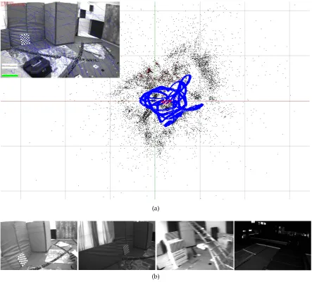
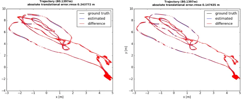
(a)

(b)

Figure 2.(a) is the result of proposed system for V1 02 in EuRoC benchmark dataset, blue line is the estimated trajectory, black dots show reconstructed sparse landmarks, and red square represents the current camera pose. (b) shows a captured camera images in the EuRoC, which has experience of challenging environmental changes such as motion blur and illumination changes. Our proposed system has been verified to be able to estimate reliable poses for all sequences in Section6.

4. Visual inertial optimization

The goal of the visual-inertial odometer is to estimate the current motional state using visual information and inertial measurements at every time. The statestat timetis defined as a quadruple

st=hw_dTt,wvt,dbat,dbωti, (1)

where,w_dT= [w_dR,wp]∈SE(3)is the transformation from the device to the world coordinate system, vis the velocity of the device, anddba_,d_bω _{are the sensor bias. The coordinate systems are denoted as}

a prescript on the left side of the symbol, and there are the world (w), the device (d), and the camera (c) coordinate systems. The time is denoted as a subscript (t) of the symbol. The world coordinate system is defined so that the gravity direction is aligned with the negativez-axis. We follow the convention that the device coordinate system is aligned with the IMU coordinate system. The transformation from the camera to the device coordinate system is written asdcTand it is pre-calculated in the device

4.1. Visual reprojection error

The visual error term of our proposed method uses the re-projection error in the conventional local bundle adjustment. The error is the difference between the projected locationxi,lof a 3D landmarkXl and its tracked location ˆxi,lat the keyframei. The visual costC_kν_,ifrom the tracked features is defined as:

Cν k,i=ρ

eν_(i,l)>Λν i,leν(i,l)

(2)

eν_{(i,l) =xˆ} i,l−π

d

cT−1?wdT−1?wXl

, (3)

whereΛν

i,lis the information matrix associated with the tracked feature point at the keyframe, and

πdenotes the camera projection function. ?and−1denotes the composition/application and the

inversion operators for SE(3) transformations respectively, andρis the Huber norm [27], which is

defined as:

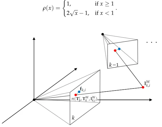
ρ(x) = (

1, ifx≥1

2√x−1, ifx<1. (4)

−1

. . .

Figure 3.Visualization of visual error. The green dashed line represents re-projection erroreν_and

visual error term optimizes the summation of these errors for local window.

4.2. IMU Pre-Integration

The IMU sensors measure the angular velocity and translational acceleration and in theory the 3D pose (orientation and position) of the device can be calculated by integrating the sensor readings over time. However, the raw IMU measurements contain significant noise and time-varying non-zero bias, and these make the integration-based pose estimation very challenging. The IMU angular velocitydωˆ and accelerationdaˆmeasurements at timetare modeled with the true accelerationwaand angular velocitydωas

d_aˆ

t=w_dR>t (wat−wg) +dbat+na, and (5)

d_ˆ

ωt=dωt+dbωt+nω, (6)

wherew_dR>_t is the rotation from the world to the device coordinates (note the transpose),wgis the constant gravity vector in the world,dbat,dbω

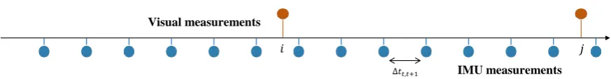
𝑖 𝑗

∆𝑡𝑡,𝑡+1

Visual measurements

IMU measurements

Figure 4.IMU sensor measurements are typically much faster than the camera frame rate. In this study, we verified the algorithm using a 200Hz IMU sensor and a 20fps camera on the EuRoC benchmark dataset, whereiandjare the camera capture time andtis the IMU measurement time.



 

w_{p˙ =}w_v

w_{v˙ =}w_a

w_˙

R=w_dR[dω]× 



, where [ω]×= 

 

0 −ωz ωy

ωz 0 −ωx

−ωy ωx 0





, (7)

for the image frameskandk+1 (at timetkandtk+1respectively), the position, velocity, and

orientation of the device can be propagated through the first and second-integration used in [28],

w_p

k+1=wpk+wvk∆tk+ Z Z

t∈tk,tk+1

(w_dRt(daˆt−dbat−na) +wg)dt2 (8)

w_v

k+1=wvk+ Z

t∈t_k,t_k+1

(w_dRt(daˆt−dbat−na) +wg)dt (9)

w

dRk+1=wdRkExp

Z

t∈tk,tk+1

(dωˆt−dbωt−nω)dt

. (10)

Assuming the accelerationdaˆkand the angular velocitydωˆkare constant between time intervaltk andtk+1, we can simplify the above equations as follows:

w_p

k+1=wpk+wvk∆tk,k+1+1

2

w_g∆t2

k,k+1+

1 2

w dRtk(

d_aˆ

t_k−dbat_k−na)∆t2_k,k+1 (11)

w_v

k+1=wvk+wg∆tk,k+1+wdRtk( d_aˆ

tk− d

batk−n a_)∆tk

,k+1 (12)

w

dRk+1=wdRtkExp

(dωˆt_k−dbωt_k−nω)∆tk,k+1

. (13)

The measurement rate of the IMU is much faster than that of the camera, as illustrated in Figure4, and it is computationally burdensome to re-integrate the values according to the changes of the state in the optimization framework. Thus, we follow the pre-integration method, which represents IMU measurements to the poses of the consecutive frames by adding IMU factors incrementally as in [7,8].

For two consecutive keyframes [i,j] where the time between two (ti,tj) can vary, the changes of position, velocity, and orientation that are not dependent to the biases can be written as follows from the Equations11-13:

∆pi,j := wdR

>

i (wpj−wpi−wvi∆ti,j− 1 2

w_g∆t2

i,j) = j−1

∑

k=i 1 2R

i k(daˆtk−

d

bat_k−na)∆t2_k,k+1 (14)

∆vi,j := wdR

>

i (wvj−wvi−wg∆ti,j) = j−1

∑

k=i

Ri_k(daˆt_k−dbat_k−na)∆tk,k+1 (15)

∆Ri,j := (wdRi)>wdRj = j−1

∏

k=i

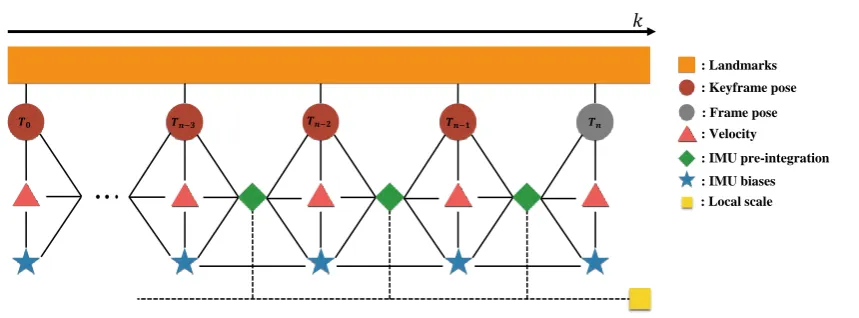
: Velocity

: IMU pre-integration

: IMU biases : Landmarks : Keyframe pose

: Frame pose

𝑻𝒏−𝟐 𝑻𝒏−𝟏

𝑻𝟎 𝑻𝒏−𝟑 𝑻𝒏

𝑘

: Local scale

Figure 5. Illustration of the proposed visual inertial local bundle adjustment. All keyframe poses hw_dT0,w_dT1, . . . ,w_dTnicontain visual terms with landmarks and IMU pre-integration factor with local scale variable. The current framen is included in the local window with the accumulated IMU pre-integration.

whereRi_k represents the rotation from the framekto the timei. We can calculate the right side of above equation directly from the IMU measurements and the biases between the two keyframes. However, these equations are the function of the biasdbatk and

d_bω

tk. If the biases

d_ba_andd_bω

between the keyframes are assumed to be fixed, we can obtain the values of∆pi,j,∆vi,j,∆Ri,jfrom the IMU measurements without re-integration.

However, in the case of bias, it changes slightly in the optimization window, and we use recent IMU pre-integration described in [7,8] to reflect the bias changes in the optimization by updating delta measurements of bias using the Jacobians which describe how the measurements change due to the estimation of the bias, as

w_p

j=wpi+wvi∆ti,j+1 2

w_g∆t2

i,j+wdRi(∆pi,j+Jω_∆p

d bω

i+Ja_∆p

d

bai) (17)

w_v

j=wvi+wg∆ti,j+wdRi(∆vi,j+Jω_∆vdbωi+Ja_∆vdbai) (18)

w

dRj=wdRi∆Ri,jExp(Jω_∆R

d bω

i), (19)

whereJaandJω _{are the Jacobians which are first-order approximations of the variation of the IMU}

biases.

Finally, the local optimization cost of the IMU residualeµ_i,jfor the interval of keyframesiandj using pre-integration is defined as follows:

Cµ

i,j=eµ(i,j)

>_Λµ

i,jeµ(i,j) (20)

eµ_{(i,j) =}

        w

dR>i (wpj−wpi−wvi∆ti,j−1₂wg∆t2_i,j)−(∆pi,j+Jω_∆pdbωi+Ja_∆pdbai)

w

dR>i (wvj−wvi−wg∆ti,j)−(∆vi,j+Jω_∆vdbωi+Ja_∆vdbai) Log((∆Ri,jExp(Jω_∆Rdbωi))>(wdRi)>wdRj)

d_ba j−dbai

d_bω

j−dbωi

        (21)

Considering UAVs, the VIO system should estimate the current pose in real-time using captured visual information and IMU measurement. We use the visual-inertial bundle adjustment framework and solve the optimization problem with the Gauss-Newton algorithm implemented in the ceres-solver [29]. For the state sn and the 3D landmarks lm, the cost function is defined as follows for the optimization window

Sonline =hs0,s1, . . .sn,lmi (22)

S∗online=argmin Sonline

(

Cρ₊

∑

Cν k,i+

∑

k

Cµ k,k+1

)

k∈[0,n],i∈m (23)

where,Cρ_{is the prior information from marginalization which is the factor for the states out of the} local optimization window.

The scale estimated from initialization is often not observable since it has a dependent on motion. In order to estimate a optimal metric scale, we include the local scale factor into our cost function and optimize it with other variables such as poses. When a new keyframe is added, we assumed that the device experiences the motion changes and perform jointly optimization including local scales variable.

eµ_{(i,j) =}



      

w

dR>i ((wpj−wpi)s−wvi∆ti,j−12wg∆t2i,j)−(∆pi,j+Jω_∆p

d_bω

i+Ja_∆p

d_ba i)

w

dRi>(wvj−wvi−wg∆ti,j)−(∆vi,j+Jω_∆v

d_bω

i+Ja_∆v

d_ba i) Log((∆Ri,jExp(Jω_∆R

d_bω

i))>(wdRi)>wdRj)

d_ba

j−dbai

d_bω

j−dbωi



      

(24)

Figure5shows the graphical model of our visual inertial local bundle adjustment. We perform local optimization with sufficiently accurate scale variable which is computed through bootstrapping in Section5, and the optimized reliable local scale is marginalized to prior information along with the pose of the old keyframe.

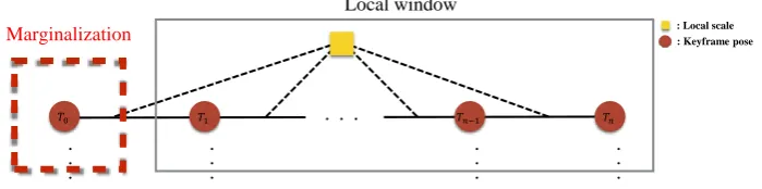
4.4. Marginalization

The optimization-based VIO algorithms need to marginalize out the old information not to slow down the processing speed [5,7]. The marginalization does not eliminate the old information outside of the local optimization window of keyframes, but converts it into a linearized approximate form to the remaining state variables using Schur complement [30]. When a new keyframe is added into the local optimization window and the window size exceeds the preset threshold, the state of the oldest keyframe in the window including the pose, velocity, and bias is marginalized (Figure 7illustrates keyframe marginalization in a graphical model). On the other hand, if the current frame is not selected as a keyframe, only the visual information is dropped while the IMU measurements are kept for IMU pre-integration. The marginalized factor is applied to be a prior of the next optimization, which helps to find a better solution than simply fixing the keyframe poses outside of the optimization window.

Local window

𝑇0 𝑇1 . . . 𝑇𝑛−1 𝑇𝑛

Marginalization

.

. . . .

: Local scale : Keyframe pose

Figure 7.Old keyframe marginalization with optimized scale. Marginalized measurements are used as prior for the next optimization.

5. Bootstrapping

Unlike the monocular visual odometry where the camera parameters are known and the absolute scale of the map is not recoverable, the visual-inertial odometry needs to find the critical parameters such as the scale of the map and gravity direction to robustly estimate the state. Moreover there are many motion patterns in which the multiple solutions of IMU bias parameters exist, such as constant velocity motions including no motion [9]; thus, optimization involving all state variables without precise initialization may not converge to the true solution. For these reasons, some VIO systems require approximate manual initialization of the gravity vectors or IMU biases, or real scale distance information using different sensors [31]. The map of visual features are constructed starting from the two keyframes with sufficient parallax, and it is continuously updated as more keyframes are observed. However, the IMU measurements for these keyframes may not observe any significant changes in acceleration, and this can cause failure in bootstrapping the VIO system.

In this work, we propose a bootstrapping method that computes the accurate scale and gravity through stepwise optimization using relative pose constraints. Our method consists of vision-only map building, pose graph optimization with IMU pre-integration, convergence check, and IMU bias update.

5.1. Vision-only map building

The first step, vison-only map building, is identical to monocular visual odometry [32,33] and structure from motion algorithms (SFM) [34]. The system finds the first two keyframeswcT0and w

cT1 with sufficient motion, by checking the numbers of inlier features by a Homography and a

Data:Images, accelerations and gyro Result:6DOF poses and landmarks

Initialization : Select 2 keyframes for visual motion based initialization and perform visual odometry to estimate relative keyframe motion [37]. Then, calculate the metric scale and gravity by PGO with IMU factor. Check the convergence of the optimized parameters and re-propagate the pre-integration factor using the initial bias, scale and gravity;

for k = 1 to Kdo

Extract and tracking keypoints using KLT [20]; if kthframe is keyframethen

Add new landmarks;

Perform online optimization minimizing cost function with local scale factor Eqn.24; Marginalize old keyframe’s variables with scale.;

else

Performs pose optimization by Eqn.22with fixed previous keyframe’s poses; Marginalize visual information observed on current frame;

end end

returnoptimized 6DOF pose and landmarks involving real scale

built the pose of later keyframes are computed by the PNP algorithm [36] Local bundle adjustment using Equation2is performed initially and whenever a keyframe is added to improve the accuracy of pose and point positions. Until the scale and gravity is reliably measured in the next steps, purely vision-only map building is continued.

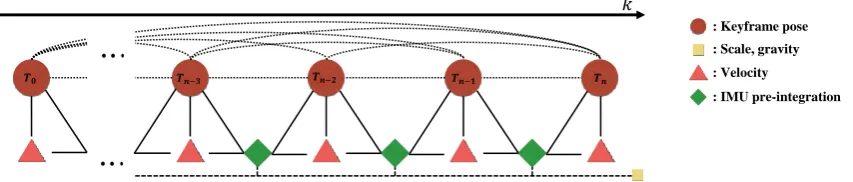
5.2. Pose graph optimization with IMU pre-integration

While purely visual mapping is running, we try to estimate the metric scale using the pre-integrated IMU factor. For easy formulation and efficient estimation, we adopt the pose graph optimization (PGO) framework [19,38,39] which constructs a graph of keyframes whose edges represent the relative pose constraints between keyframes, and optimizes the keyframe poses so that the inconsistency of the relative poses and constraints are minimized (note that this is equivalent to marginalizing the landmarks in bundle adjustment). PGO is commonly used in monocular SLAM systems to fix the scale drift in loop closures using Sim(3) relative poses. In contrast we use SE(3) relative poses with a global scale parametersto the entire map, as the scale drift for a short period of initialization time is not significant. Additional constraints from the pre-integrated IMU and the gravity vector are added to PGO, and the factors in our formulation are illustrated in Figure8.

Formally we define the state for PGO with all keyframe poses, velocities, the gravity, and the global scalesas

Spgo =hwT0,wT1, . . . ,wTn,wT0,wv1, . . . ,wvn,wg,si. (25)

In this section we parameterize an SE(3) transformation with a pair of a translation vectorpand a Hamiltonian quaternion [40]q, i.e.,T= [R(q),p], whereR(·)is the function converting a quaternion to a 3×3 rotation matrix.

While performing visual pose estimation, we calculate IMU pre-integration for keyframes using Equations 17-19, in which bias and noise are initialized as zero. Using Equations17-18for consecutive keyframesiandj, we obtain the scale error costes_i,j

C_is_,j= (es(i,j))>Λs_i,jes(i,j) (26)

es(i,j) =

"

R(w_q

i)>((wpj−wpi)s−wvi∆ti,j−12wg∆t2i,j)−(∆pi,j+Jω_∆p

d bω

i+J_∆apdbai)

R(w_q

i)>(wvj−wvi−wg∆ti,j)−(∆vi,j+Jω_∆vdbωi+Ja_∆vdbai)

#

: Velocity

: IMU pre-integration : Keyframe pose 𝑘

𝑻𝒏−𝟐 𝑻𝒏−𝟏

𝑻𝟎 𝑻𝒏−𝟑 𝑻𝒏

: Scale, gravity

Figure 8.Proposed pose graph optimization model including metric scale and gravity variables. We estimate the metric scale and gravity while maintaining the fundamental relationship of the relative pose for whole keyframes.

Hereby,Λs_i,j denotes the information matrix, and we use the sub-block ofΛµ_i,j. Experimentally, the metric scale can be calculated to be zero if the motion is partially small or involve no motion. To prevent this case, the scale factor in the proposed method uses exponential parameterization.

For the relative pose between two keyframesiandjis given aspi,j = R(qi)(wpj−wpi)and qi,j =w_dq∗i wdqj, the relative pose costs in PGO are given as follows:

C_irel_,j =erel(i,j)>Λrel_i,jerel(i,j) (28)

erel(i,j) =

"

pi,j−pˆi,j 2 ∗Vec(qi,jqˆ∗i,j)

#

(29)

where ( ˆpi,j, ˆqi,j) is the relative pose constraint between keyframeiandjin the current map, Vec(q)

returns the vector (imaginary) part of theqandΛrel_i,j is the information matrix from the keyframe pose covariance.

We define the optimization cost for a new stateSpgoby combining Equations29and 26for whole keyframesnas follows:

S∗pgo=argmin Spgo

(

∑

i,j∈k

Creli,j+

∑

C_ks_,k+1

)

, k∈[0,n]. (30)

Note that, because we know that the magnitude of gravitygis 9.8, we include the constraintg>g=9.82 when performing the optimization.

5.3. Convergence check

The proposed scale and gravity optimization can be calculated in real-time at the moment of insertion of a new keyframe, and we update the optimized variable at a point sufficient to initialize VIO. We use two ways to measure the accuracy: covariance ofX∗and variance of optimized scale variables. The covariance ofS∗pgois given by,

C(S∗pgo) =

J>(S∗pgo)J(S∗pgo)

−1

(31)

whereJ(S∗pgo)is the Jacobian of Equation30atS∗pgo. We apply the optimized scale and gravity to the system initialization when the largest eigenvalue of the optimized covarianceλmax(C(S∗pgo))is less than the thresholdτcovand the scale variance is less than the thresholdτvarat the same time. The scale

Figure 9.The optimized scale variable for the sequence MH 01. The optimal scale value is computed aligning the estimated trajectory with the ground-truth via Sim(3)[41]. Our bootstrapping algorithm estimate reliable initial scale within the 50-th frame, then optimizes the local scale to the optimal value by Eqn.24and update incrementally.

5.4. IMU biases update

After the optimized scale and gravity are applied to stateS, we can calculate the initial IMU biases while fixing the pose variableshwT0,wT1, . . . ,wTkiin the optimization using Equation22. The pre-integration factors for the local window keyframes are re-propagated using biases computed through initialization. At this point, the bootstrapping of the VIO is complete and online optimization is performed using the framework presented in Section4.3.

6. Experiments

We used the EuRoC [10] dataset, which contains various challenging motions, to evaluate the quantitative performance of the proposed algorithm. The dataset was collected from a "Firefly" micro-aerial vehicle equipped with a stereo camera and inertial measurement at high flying speeds. We used only the left images with inertial sensor data. The sensor data in the EuRoC dataset were captured as a global shutter WVGA monochrome image at 20 fps and IMU data at 200 Hz. This dataset consists of five "Machine Hall" sequences and six "Vicon Room" sequences, which are labeled into easy, normal and difficult, depending on the motion speed and illumination environment changes. Both types of datasets measure the ground truth position from the Leica MS50 laser tracker and Vicon motion capture systems and are well calibrated to be used as benchmark datasets in various SLAM applications. We implemented the proposed system in C ++ without GPU and was executed it on Intel Core i7 3.0G CPU laptops with 16GB RAM in real-time.

6.1. Comparison

We compared our proposed algorithm with recent state-of-the-art approaches using the same evaluation method as Delmerico and Scaramuzza [31], who evaluated the benchmark VIO performance in advance. They used the recommended parameter settings maintained in all tests of each algorithm and evaluated the RMSE position error over the align trajectory to ground truth pose via SE(3)[42]. Note that, because our proposed method is not a SLAM system, we conducted the comparison evaluation with algorithms that do not include loop closing. We directly compared the RMSE results with OKVIS [5], ROVIO [43], VINS-Mono [17], SVO+MSF [44,45] and SVO+GTSAM [46] using [31].

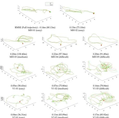
RMSE (Full trajectory) : 0.14m (80.13m) 0.13m (73.10m)

MH 01 (easy) MH 02 (easy)

0.20m (130.40m) 0.22m (97.34m) 0.20m (91.49m)

MH 03 (medium) MH 04 (difficult) MH 05 (difficult)

0.05m (58.43m) 0.07m (75.80m) 0.16m (78.84m)

V1 01 (easy) V1 02 (medium) V1 03 (difficult)

0.04m (36.31m) 0.11m (83.09m) 0.17m (85.92m)

V2 01 (easy) V2 02 (medium) V2 03 (difficult)

Figure 10. Trajectory result of the proposed method and ground truth. Estimated trajectories are aligned to ground truth pose via SE(3). The green line represents ground truth trajectory and the red dashed line is ours. For overall sequences, the proposed method estimates the accurate poses without any failure cases in tightly coupled optimization framework with a robust initialization method using relative pose constraints.

visual patches and IMU measurement with EKF framework. Note that, this VIO system needs manual initialization using extra sensors. SVO+GTSM optimize structureless visual reprojection error with IMU pre-integration term performing full-smoothing factor graph optimization by [14]. These several methods differ from visual term (re-projection and photometric error), IMU term (IMU pre-integration and direct integration) and minimization method. Since the VIO system is a pose estimation method in continuous situations that does not involve re-localization, partial pose estimation failures can not be restored in extreme environments changes such as fast motion or dramatic illumination changes (V1 03 (difficult), V2 03 (difficult)).

EuRoC seq Ours SVO+MSF [45] OKVIS [5] ROVIO [43] VINS-MONO [17] SVO+GTSAM [46]

MH 01 (easy) 0.14 0.14 0.16 0.21 0.27 0.05

MH 02 (easy) 0.13 0.20 0.22 0.25 0.12 0.03

MH 03 (medium) 0.20 0.48 0.24 0.25 0.13 0.12

MH 04 (difficult) 0.22 1.38 0.34 0.49 0.23 0.13

MH 05 (difficult) 0.20 0.51 0.47 0.52 0.35 0.16

V1 01 (easy) 0.05 0.40 0.09 0.10 0.07 0.07

V1 02 (medium) 0.07 0.63 0.20 0.10 0.10 0.11

V1 03 (difficult) 0.16 X 0.24 0.14 0.13 X

V2 01 (easy) 0.04 0.20 0.13 0.12 0.08 0.07

V2 02 (medium) 0.11 0.37 0.16 0.14 0.08 X

V2 03 (difficult) 0.17 X 0.29 0.14 0.21 X

Overall 0.13 0.23 0.22 0.16

works well with the same parameters for whole sequences without any failures. ROVIO, VINS and OKVIS operate robustly in all sequences, but get low accuracy at V2 03, which is difficult to robust initialization due to fast motion and MH 05 which contains night-time outdoor scene. SVO+GTSAM makes a challenging performance in the "Machine Hall" with far features with illumination changes, however it fails to estimate temporal poses on "Vicon Room" including fast motion (V1 03, V2 02-03). Our algorithm performs well in the MH 04-05 and V1-2 03 which are the most difficult dataset with dramatic illumination changes involving motion blur and darkness scene. Accurate scale and gravity initialization can reliably update the bias, and it is also possible to estimate exact pose in unstable feature tracking case through continuous scale updating. We make the best performance for overall without any failure cases in tightly coupled optimization framework with a robust initialization method using relative pose constraints. The most important aspect of the UAVs is to estimate the pose stably for the entire running without other extra sensors. The proposed method suited for this since it uses all the visual observation of the previous state by calculating the global metric scale and gravity while stably estimating the pose using visual information from the start.

7. Conclusions

In this paper, we propose a stable and accurate monocular visual inertial odometry system, which can be applied to UAVs in unknown environments. Even when we do not know the initial motion well, we optimize the relative motion with the IMU pre-integration factor to effectively solve the high non-linear problem and estimate reliable states by performing jointly optimization. We also estimate the local scale and update it into the marginalization to overcome the limitation of the sliding window approach where the observations are reduced. Further, We present that our proposed method makes stable and accurate results for EuRoC benchmark dataset experiencing various environmental changes.

Author Contributions:E.H. implemented the system and write original draft preparation with validation. And J.L. conceived main methodology and supervise with editing the manuscript. All authors read and approved the final manuscript.

Funding: This research was supported by Next-Generation Information Computing Development Program through the National Research Foundation of Korea(NRF) funded by the Ministry of Science, ICT (NRF-2017M3C4A7069369) and the National Research Foundation of Korea(NRF) grant funded by the Korea government(MISP)(NRF-2017R1A2B4011928).

Conflicts of Interest:The authors declare no conflict of interest.

1. Weiss, S.; Achtelik, M.W.; Lynen, S.; Chli, M.; Siegwart, R. Real-time onboard visual-inertial state estimation and self-calibration of mavs in unknown environments. Robotics and Automation (ICRA), 2012 IEEE International Conference on. IEEE, 2012, pp. 957–964.

2. Lynen, S.; Achtelik, M.W.; Weiss, S.; Chli, M.; Siegwart, R. A robust and modular multi-sensor fusion approach applied to mav navigation. Intelligent Robots and Systems (IROS), 2013 IEEE/RSJ International Conference on. IEEE, 2013, pp. 3923–3929.

3. Mourikis, A.I.; Roumeliotis, S.I. A multi-state constraint Kalman filter for vision-aided inertial navigation. Proceedings 2007 IEEE International Conference on Robotics and Automation. IEEE, 2007, pp. 3565–3572. 4. Li, M.; Mourikis, A.I. High-precision, consistent EKF-based visual–inertial odometry. The International

Journal of Robotics Research2013,32, 690–711.

5. Leutenegger, S.; Lynen, S.; Bosse, M.; Siegwart, R.; Furgale, P. Keyframe-based visual–inertial odometry using nonlinear optimization.The International Journal of Robotics Research2015,34, 314–334.

6. Mur-Artal, R.; Tardós, J.D. Visual-inertial monocular SLAM with map reuse.IEEE Robotics and Automation Letters2017,2, 796–803.

7. Qin, T.; Li, P.; Shen, S. Vins-mono: A robust and versatile monocular visual-inertial state estimator. IEEE Transactions on Robotics2018, pp. 1–17.

8. Forster, C.; Carlone, L.; Dellaert, F.; Scaramuzza, D. On-Manifold Preintegration Theory for Fast and Accurate Visual-Inertial Navigation. arXiv preprint arXiv:1512.023632015.

9. Martinelli, A. Closed-form solution of visual-inertial structure from motion.International journal of computer vision2014,106, 138–152.

10. Burri, M.; Nikolic, J.; Gohl, P.; Schneider, T.; Rehder, J.; Omari, S.; Achtelik, M.W.; Siegwart, R. The EuRoC micro aerial vehicle datasets. The International Journal of Robotics Research2016, p. 0278364915620033. 11. Ljung, L. Asymptotic behavior of the extended Kalman filter as a parameter estimator for linear systems.

IEEE Transactions on Automatic Control1979,24, 36–50.

12. Hesch, J.A.; Kottas, D.G.; Bowman, S.L.; Roumeliotis, S.I. Consistency analysis and improvement of vision-aided inertial navigation.IEEE Transactions on Robotics2014,30, 158–176.

13. Mouragnon, E.; Lhuillier, M.; Dhome, M.; Dekeyser, F.; Sayd, P. Generic and real-time structure from motion using local bundle adjustment. Image and Vision Computing2009,27, 1178–1193.

14. Kaess, M.; Johannsson, H.; Roberts, R.; Ila, V.; Leonard, J.J.; Dellaert, F. iSAM2: Incremental smoothing and mapping using the Bayes tree. The International Journal of Robotics Research2011, p. 0278364911430419. 15. Lupton, T.; Sukkarieh, S. Visual-inertial-aided navigation for high-dynamic motion in built environments

without initial conditions. IEEE Transactions on Robotics2012,28, 61–76.

16. Shen, S.; Michael, N.; Kumar, V. Tightly-coupled monocular visual-inertial fusion for autonomous flight of rotorcraft MAVs. Robotics and Automation (ICRA), 2015 IEEE International Conference on. IEEE, 2015, pp. 5303–5310.

17. Qin, T.; Shen, S. Robust initialization of monocular visual-inertial estimation on aerial robots. Intelligent Robots and Systems (IROS), 2017 IEEE/RSJ International Conference on. IEEE, 2017, pp. 4225–4232. 18. Weiss, S.; Brockers, R.; Albrektsen, S.; Matthies, L. Inertial optical flow for throw-and-go micro air vehicles.

Applications of Computer Vision (WACV), 2015 IEEE Winter Conference on. IEEE, 2015, pp. 262–269. 19. Sibley, D.; Mei, C.; Reid, I.D.; Newman, P. Adaptive relative bundle adjustment. Robotics: science and

systems, 2009, Vol. 32, p. 33.

2003,31, 3812–3814.

22. Bay, H.; Tuytelaars, T.; Van Gool, L. Surf: Speeded up robust features. European conference on computer vision. Springer, 2006, pp. 404–417.

23. Calonder, M.; Lepetit, V.; Strecha, C.; Fua, P. Brief: Binary robust independent elementary features. European conference on computer vision. Springer, 2010, pp. 778–792.

24. Rublee, E.; Rabaud, V.; Konolige, K.; Bradski, G. ORB: An efficient alternative to SIFT or SURF. 2011 International conference on computer vision. IEEE, 2011, pp. 2564–2571.

25. Rehder, J.; Nikolic, J.; Schneider, T.; Hinzmann, T.; Siegwart, R. Extending kalibr: Calibrating the extrinsics of multiple IMUs and of individual axes. Robotics and Automation (ICRA), 2016 IEEE International Conference on. IEEE, 2016, pp. 4304–4311.

26. Furgale, P.; Rehder, J.; Siegwart, R. Unified temporal and spatial calibration for multi-sensor systems. Intelligent Robots and Systems (IROS), 2013 IEEE/RSJ International Conference on. IEEE, 2013, pp. 1280–1286.

27. Huber, P.J.; others. Robust estimation of a location parameter. The annals of mathematical statistics1964, 35, 73–101.

28. Farrell, J.Aided navigation: GPS with high rate sensors; McGraw-Hill, Inc., 2008. 29. Agarwal, S.; Mierle, K.; Others. Ceres Solver. http://ceres-solver.org. 30. Jin, J.M.The finite element method in electromagnetics; John Wiley & Sons, 2015.

31. Delmerico, J.; Scaramuzza, D. A Benchmark Comparison of Monocular Visual-Inertial Odometry Algorithms for Flying Robots.Memory2018,10, 20.

32. Engel, J.; Schöps, T.; Cremers, D. LSD-SLAM: Large-scale direct monocular SLAM. European Conference on Computer Vision. Springer, 2014, pp. 834–849.

33. Mur-Artal, R.; Montiel, J.M.M.; Tardos, J.D. ORB-SLAM: a versatile and accurate monocular SLAM system. IEEE Transactions on Robotics2015,31, 1147–1163.

34. Sturm, P.; Triggs, B. A factorization based algorithm for multi-image projective structure and motion. European conference on computer vision. Springer, 1996, pp. 709–720.

35. Nistér, D. An efficient solution to the five-point relative pose problem.IEEE transactions on pattern analysis and machine intelligence2004,26, 756–770.

36. Lepetit, V.; Moreno-Noguer, F.; Fua, P. Epnp: An accurate o (n) solution to the pnp problem. International journal of computer vision2009,81, 155.

37. Westoby, M.J.; Brasington, J.; Glasser, N.F.; Hambrey, M.J.; Reynolds, J. ‘Structure-from-Motion’photogrammetry: A low-cost, effective tool for geoscience applications.

Geomorphology2012,179, 300–314.

38. Eustice, R.; Singh, H.; Leonard, J.J.; Walter, M.R.; Ballard, R. Visually Navigating the RMS Titanic with SLAM Information Filters. Robotics: Science and Systems, 2005, Vol. 2005, pp. 57–64.

39. Thrun, S.; Burgard, W.; Fox, D.Probabilistic robotics; MIT press, 2005.

40. Pohlmeyer, K. Integrable Hamiltonian systems and interactions through quadratic constraints. Communications in Mathematical Physics1976,46, 207–221.

41. Horn, B.K. Closed-form solution of absolute orientation using unit quaternions. JOSA A1987,4, 629–642. 42. Umeyama, S. Least-squares estimation of transformation parameters between two point patterns. IEEE

Transactions on Pattern Analysis & Machine Intelligence1991, pp. 376–380.

43. Bloesch, M.; Omari, S.; Hutter, M.; Siegwart, R. Robust visual inertial odometry using a direct EKF-based approach. Intelligent Robots and Systems (IROS), 2015 IEEE/RSJ International Conference on. IEEE, 2015, pp. 298–304.

44. Forster, C.; Zhang, Z.; Gassner, M.; Werlberger, M.; Scaramuzza, D. Svo: Semidirect visual odometry for monocular and multicamera systems. IEEE Transactions on Robotics2017,33, 249–265.

45. Faessler, M.; Fontana, F.; Forster, C.; Mueggler, E.; Pizzoli, M.; Scaramuzza, D. Autonomous, vision-based flight and live dense 3d mapping with a quadrotor micro aerial vehicle. Journal of Field Robotics2016, 33, 431–450.