Modeling the Throughput of 1-persistent CSMA
in Underwater Networks
Alain Olivier
⋆, Michele Zorzi
⋆, Paolo Casari
‡⋆
Department of Information Engineering, University of Padova, via Gradenigo 6/B, 35131 Padova, Italy ‡
IMDEA Networks Institute, Madrid, Spain
⋆{
oliviera,zorzi}@dei.unipd.it ‡[email protected]
Abstract—The aim of this paper is to present a model for the throughput of the 1-persistent CSMA protocol in underwater net-works, where the typically large propagation delay with respect to the packet transmission time requires to take into account the spatial distribution of the nodes. Our model is developed based on the analysis carried out in [1] for the non-persistent CSMA protocol. Our results show that the 1-persistent CSMA model developed by Tobagi and Kleinrock is still valid as an approximation, with a few small adjustments, even though it considers an equal propagation delay for all pairs of nodes in the network. The proposed model is validated against simulation results based on the network simulator OMNeT++.
Index Terms—Underwater acoustic networks, CSMA, Medium Access Control, throughput analysis, simulation.
I. INTRODUCTION
Carrier Sense Multiple Access (CSMA) is a Medium Access Control (MAC) protocol based on random access with channel sensing prior to each transmission. In underwater networks, CSMA has been playing a significant role mainly for two reasons:i) it is simple to implement in real hardware for field experiments, as it does not require additional capabilities such as network synchronization;ii) even when the sensing range is equal to the reception range (as is typically the case for most off-the-shelf commercial modems to date), CSMA still helps avoid some collision events, such as those caused by a node starting to transmit when it is overhearing a packet not meant for itself. Indeed, CSMA has been among the first protocols to be tested in simple MAC experiments in small networks [2]. In its collision avoidance flavor (CSMA/CA), which makes use of a preliminary 4-way handshaking, CSMA has been investigated, analyzed and simulated in different scenarios and under different assumptions, including hybrid approaches [3]. For example, the authors in [4] consider TDMA features to enhance the performance of a CSMA-based access protocol by implementing a network synchronization protocol and by having all nodes estimate the propagation delay towards all neighbors in order to predict collision events; [5] employs CSMA/CA as a MAC scheme on top of Orthog-onal Frequency-Division Multiplexing (OFDM) for multiple swarming autonomous underwater vehicles; a MACA-based protocol is proposed in [6] and analyzed by taking into ac-count the significant propagation delay of underwater acoustic channels (compared to control and data packet transmission times) and the typically severe data losses experienced under
water; a virtual full-duplex scheme exploiting the underwater acoustic propagation delay is proposed in [7] to improve the performance of CSMA/CA.
In the following, we will focus on the “sense-before-transmit” version of CSMA, i.e., without collision avoidance mechanisms based on preliminary handshakes. According to the terminology established by Tobagi and Kleinrock [8] (TK for short), in non-persistent CSMA (np-CSMA) the node backs off and reschedules a later transmission attempt whenever the channel is sensed busy.
In a more general version, named p-persistent CSMA (p-CSMA), time is slotted and a node senses the channel in each slot: if the channel is sensed idle, the node transmits with probabilityp, and refrains with probability1−p; if the channel is busy, the node backs off and performs sensing again in the next slot.
A specific version of p-persistent CSMA sets p = 1
and is named 1-persistent CSMA (1p-CSMA). The latter technique may potentially achieve better channel utilization than np-CSMA, but if two users sense the channel to be busy within a short time window, it becomes highly likely that their transmissions will collide [8].
Theoretically, CSMA makes it possible to achieve maximum channel utilizationS, defined as the ratio of the amount of time spent for correct transmissions over the total time. However, underwater networks typically exhibit large propagation delays (denoted here as τ), where “large” means that τ is a non-negligible fraction of, or may even be larger than, the packet transmission timeTD. The performance of CSMA is studied
by Tobagi and Kleinrock in [8] assuming that τ is constant across all node pairs, which is appropriate only whenτ≪TD.
the throughput whenτ is not negligible with respect toTD.
In this paper, we extend the results in [1] by analyzing the throughput and success probability performance of 1p-CSMA in networks with large propagation delays. We show that the different traffic pattern with respect to np-CSMA leads to different time-varying packet arrival rates than shown in [1] for the np-CSMA case, and discuss an approximation to these rates. The throughput analysis based on these results is shown to provide better accuracy when predicting 1p-CSMA performance figures with respect to the TK model in [8]. As introduced at the beginning of this section, our analysis is quite relevant to underwater networking, as many protocol stacks are based on some form of CSMA, possibly even natively provided by the modem [9].
The rest of this paper is organized as follows. In the next section we briefly describe the network scenario and introduce the notation used. In Section III we investigate the rates introduced by Koseoglu and Karasan in their paper [1] and characterize their behavior for large values of a. This will be the basis for the development of our model as we revisit the TK model in Section IV based on the results in Section III. In Section V, the model is compared to simulation results obtained using the OMNeT++ network simulator. Finally, in Section VI, we will discuss the model and its possible future refinements before drawing our conclusions.
II. NETWORKSCENARIO
For completeness, we now introduce the same terminology used in [8]. Let G denote the aggregate packet generation rate in the network. Let τ be the largest propagation delay of the network, and call TDthe packet transmission time. Let
a= τ
TD denote the ratio between the largest propagation delay
τ over the packet transmission timeTD.
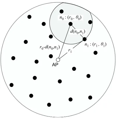
The scenario is the same as in [1] except that we assume a finite number N of users {n0, n1, . . .} to be uniformly distributed inside a circle of diameter a with the receiving access point (AP) located at the center. As in [1], we assume that physical distances and “time distances,” or propagation delays, are equivalent. From this point onward, all positions and distances considered in the model will be considered expressed in terms of time. Each node generates packets according to a Poisson process of parameter NG. The described
scenario is illustrated with reference to Fig. 1. Each node ni
of the network is located at the polar coordinates pair(ri, θi)
which is referenced to the center of the circle, where the AP is located. The distance between two nodes n0 and n1 as a function of their polar coordinates can be calculated as
d(n0, n1) = q
r2
0+r12−2r0r1cos(θ0−θ1). (1) We assume that the N users are uniformly distributed within the circle, i.e., that their polar coordinates have the following probability density functions (pdfs), for 0≤i≤N−1
fR(ri) = 2ri
a2/4, 0≤ri≤
a
2 (2)
fΘ(θi) = 1
2π, 0≤θi ≤2π . (3)
AP
d(n0,n1)
r1 r0-d(n0,n1)
n0 : (r0 , θ0)
n1 : (r1 , θ1)
Figure 1. The network scenario. Nodes are uniformly distributed inside a circle whose diameter measures a time units, normalized to the packet transmission timeTD. (Adapted from [1].)
III. CHARACTERIZATION OF PACKET RATES DURING AND AFTER RECEPTION AT THEAP
Along the lines of [1], we introduce two rates, namely
λst(t) and λend(t). The former represents the average rate of colliding packets from the beginning of the reception of a packet, transmitted by a node n0, at the AP. The latter expresses the rate of incoming packets at the AP after the completion of the reception of a packet transmitted by a node
n0. In the following, we analyze both rates in details. A. Average rate of colliding packets after packet reception:
λst(t)
The rateλst(t)represents the rate of colliding packets that would arrive at the AP when a packet sent by a node n0 is received. We set t = 0 to be the epoch when the AP begins to receive the packet from noden0. First of all, notice that, because of the finite duration of a packet transmission (1 time unit, normalized to the packet transmission timeTD),
the rateλst(t)takes non-zero values only fort∈[0,1]. Given a node n1 located at (r1, θ1), this node can collide with the transmission ofn0so far ast < d(n0, n1) +r1−r0. Another collision could take place if t > d(n0, n1) + 1 +r1−r0 but this is impossible as long as t ∈ [0,1]. Taking into account the preceding assumptions, the calculation of the rate is very similar to the one in [1], except for the limited support of the function. This leads to the following linear approximation of
λst(t):
λst(t) =
Ga−t
a if t≤min(1, a)
0 if t >min(1, a) . (4)
packet. Here we sett= 0as the epoch when the AP completes the reception of a packet sent by n0. Note that, unlike in the np-CSMA case, in 1p-CSMA a node might generate a packet while the channel is busy and withhold the transmission until the channel becomes free again.1 In the following, we will refer to this type of node as a backlogged node. Three different cases are possible:
• According to the considerations in [1], if t0 is the time when a node n0 ≡ (r0, θ0) begins its transmission, a second node n1 ≡ (r1, θ1) becomes aware that the channel is idle at timet0+d(n0, n1) + 1(the normalized packet transmission time equals 1); the transmission by
n0is fully received at the AP at timet0+r0+1: therefore, a transmission byn1 not due to backlogging (referred to as “normal” transmissions in the following) could arrive at the access point whenevert≥d(n0, n1) +r1−r0; • Any node n1 is aware of n0’s transmission for a time
interval of normalized duration 1; noden1 may become backlogged during this period: in this case, it will transmit right after n1’s transmission is over and therefore its backlogged packet will be received at the AP at time
t=d(n0, n1) +r1−r0;
• Another case must be taken into account, which does not occur if a < 1: there could be a node n1, sufficiently far from the AP, which can start its transmission before being aware of the transmission of n0and whose packet will arrive at the AP after the complete reception ofn0’s packet. This can happen as long ast < d(n0, n1) +r1−
r0−1.
Thus, we can compute the rateλend(t)as the superposition of the rates at which the three cases above occur.
C. Considerations about the rates
We remark that an equality of the kindt=d(n0, n1)+r1−
r0 represents an ellipse. In fact, rewrite the former expression asd(n0, n1) +r1=t+r0and refer to Fig. 1. Now, consider a timetand, without loss of generality, a noden0= (r0,0). The set of points(r1, θ1)that satisfy the relationshipd(n0, n1) +
r1 =t+r0= constant is an ellipse with the AP, located at
(0,0), and noden0 as foci.
It is useful to determine how much the area A(t) of this ellipse, which is a function ofr0andt, varies astincreases by an infinitesimal amount∆t. For simplicity, ignore the fact that the ellipse must be contained inside the circle with diameter
a. From basic geometry, the area of an ellipse is
A(t) =πα(t)β(t) , (5) whereα(t)is the semi-major axis, β(t)the semi-minor axis, andt=d(n0, n1) +r1−r0 as above. Recall once again that all locations and distances are expressed in terms of time. We stress that the sum of the distances from the foci is always
2α(t), and that the distance of each focus from the ellipse center isf =p
α(t)2−β(t)2.
1Along the lines of [8], we assume that the nodes can hold at most one packet in their buffer.
Normalized time,
0 1 2 3 4 5 6
∆
G(t) /
∆
t
0 0.4 0.8 1.2 1.6 2
2.4 Average offered traffic
due to backlogged packets
t
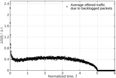
Figure 2. The average rate of incoming packets after full reception at AP due to backlogged packet fora= 5and G= 2. Notice that the function integrates toG.
In our case, the distance between the foci is constant. Therefore, we can express the area as a function oft andr0 via the following substitutions:r0+t= 2α(t)and2f(t) =r0. These lead to
α(t) = r0+t
2 ; β(t) =
s
r0+t
2
2
−r0
2
2
, (6) and the ellipse area as a function ofr0andt can be found by substituting (6) into (5). Finally, for∆tsufficiently small, we can write
∆A(t) = dA(t)
dt ∆t , (7)
where dA(t)/dt =π r2
0+ 4r0t+ 2t2/4 p
t(2r0+t). No-tice that, for t → 0 the function grows to infinity as t−1
2
and is therefore integrable. Instead, for large values of t the function grows linearly. However, since the ellipse is contained in a circle of diameter a, ∆A(t) will be constantly 0 for
t > a. Recalling that the users are uniformly distributed inside a circle of diametera, asN → ∞, an area∆A(t)will offer a traffic
∆G(t) = 4G
πa2∆A(t) . (8) Because of the linear relation between ∆A(t) and ∆G(t)
in (8), the rate due to backlogged users will assume the behavior described by Eq. (7), at least whent≪a.
In Fig. 2, we show ∆G(t)/∆tvs. tfora= 5andG= 2, by also considering the only portion of the ellipse contained inside the circle of diameteraaround the AP, and by averaging overr0. In the figure, we observe the asymptotic behavior for
t→0that has been discussed above, and also that the rate is exactly0fort > a. We note thata= 5may be representative of an underwater network where nodes communicate 100-Byte packets at 1 kbps over a maximum network radius of 2 km (assuming the propagation delay to be constant and equal to 1.5 km/s as a first-order approximation).
Normalized time,
0 1 2 3 4 5 6
0 0.5 1 1.5 2 2.5 3
Sim. λst(t)
Sim. λend(t)
λ
st(
t
)
,
λ
e
n
d(
t
)
t
Figure 3. The simulation results forλst
(t) andλend
(t)fora = 5and
G= 2.
of newly generated packets is possible for t > d(n0, n1) +
r1−r0 and also for t < d(n0, n1) +r1−r0−1. The first inequality describes the area inside the ellipse determined by the equation t = d(n0, n1) +r1−r0, whereas the second inequality describes the area outside the ellipse determined by
t=d(n0, n1) +r1−r0−1. By calling this areaE, we have
4E/(πa2)G→Gfora→+∞.
Fig. 3 shows the simulated values of λst(t) and λend(t). From the plot of λend(t), we can observe the effect of the backlogged transmission for small values of t, and also the fact that up to t=athe rate is quite close to G. In addition, we note that the simulation ofλst(t)is very well approximated by the model in (4).
D. Asymptotic Behavior
We start by analyzing the rateλst(t). Asagrows to infinity, it can be easily seen that λst(t) uniformly converges to the function:
λst(t)→λst∞(t) = (
G, 0≤t≤1
0, otherwise for a→ ∞ . (9) For the rate λend(t), we have the following considerations. First of all, from Eqs. (7) and (8), we notice that ∆G(t) is directly proportional to G; moreover, noting that the average value ofr0 is directly proportional toa(the average value of
r0 for a node uniformly distributed inside a circle is one third of the diameter,ain this case),∆G(t)is inversely proportional to the square root of a and therefore the contribution of backlogged users becomes negligible when a is large. Thus, recalling the argument about the contribution of nodesnisuch
thatt > d(n0, n1) +r1−r0 ort < d(n0, n1) +r1−r0−1, fora→ ∞, we can state thatλend(t)approaches a unit step multiplied by the rateG, that is:
λend(t)→λend∞ (t) = (
G, t≥0
0, otherwise for a→ ∞ . (10)
BUSY PERIOD
NORMALIZED TIME UNSUCCESSFUL
TRANSMISSION PERIOD
IDLE PERIOD UNSUCCESSFUL
TRANSMISSION PERIOD
SUCCESSFUL TRANSMISSION
PERIOD
1 ξ
ξ 1 Y
a
t
Figure 4. Sample case for 1-persistent CSMA: transmission periods, busy periods, and idle periods. (Adapted from [8].)
Based on these two considerations, we make the following two working assumptions:
• the rateλst(t)is constant during the packet transmission time, i.e., even though the spatial distribution is taken into account, it behaves as though nodes exhibit a common propagation delay equal to 1; along the lines of [8], this is equivalent to assuming that the vulnerable period (VP) has length 1 ifa≥1;
• the expression for the average idle period time assumes the same form as in [8].
IV. DERIVATION OF THE PROPOSED MODEL
Based on the considerations developed in Section III-D, it becomes reasonable to derive an analytical model based on the one by Tobagi and Kleinrock. From now on we refer to the analysis in [8] with a few adjustments, and we assumea≥1, which is very often the case in underwater networks.
The throughput analysis makes use of renewal theory con-cepts. The throughputS can be expressed as a function of the offered traffic Gas:
S(G) =GPs(G) , (11)
wherePsrepresents the success probability for a single packet
transmission. As claimed in [8], a packet can be successful in two cases:
1) a users begins its Transmission Period (TP) when no other user is transmitting, and none of them begin their transmission during the VP of the transmission; 2) a packet arrives during another user’s transmission and
it is the only packet arriving in this period; moreover, its sender will be the only node beginning a transmission when the channel becomes idle, and no other transmis-sion takes place during the VP of this new transmistransmis-sion. This is the situation depicted in Fig. 4 for the successful TP.
accurate forasufficiently large. Therefore, by definingI¯,B¯,
¯
B′ as in [8] and letting C¯ = ¯I+ ¯B we have the following expression forPs:
Ps(G) = ¯
I
¯
CP0+
¯
B′
¯
Cqˆ0P0+
¯
B′
¯
C(1−qˆ0)Ps(G) , (12)
whereP0is the probability of having no arrivals during the VP andqˆ0 is the probability of having no arrivals during the slot in which the packet is waiting for the channel to become idle. Note that, for simplicity, we have dropped the dependence of all terms onG. Eq. (12) yields
Ps=P0
¯
I+ ¯B′qˆ 0
¯
B−B¯′(1−qˆ 0) + ¯I
. (13) The length of the average idle period is found as
¯
I=
Z ∞
0
exp
−
Z t
0
λend∞ (u) du
dt= 1
G , (14)
where we have considered λend(t) in its asymptotic form
λend ∞ (t).
There remain to evaluate the other quantities in Eq. (11). Because λst(t)is constantly equal to Gint∈[0,1], i.e., the VP has length 1, we have
P0= exp
−
Z ∞
0
λst∞(t)dt
=e−G . (15) The distribution of the time of the last colliding transmission occurring during the VP is:
FY(t) =e−G(1−t) for t≤1 , (16)
and
¯
Y = 1− 1
G 1−e
−G
. (17) The probability of having no arrivals during transmissions in a TP is
q0=e−2G(1 +G) . (18) The average duration of a TP is
¯
T = 1 + ¯Y + ¯ξ , (19) where ξ¯ is the average time that elapses at the AP from the end of the reception of the colliding transmission to the beginning of a new transmission due to a backlogged user. In the following, we assume ξ¯to be equal to the vulnerability period at the AP, i.e., ξ¯ = 1. As proven by the results in Section V, the impact of this approximation is negligible.
We can now derive the value of the busy period (BP)B¯ (that counts the total duration of all TPs in a cycle), and the value of the BP B¯′ (that does not include the intervals of duration
ξ in each TP where the AP is not receiving. We have:
¯
B= 2 + ¯Y
q0 ,
¯
B′= 1 + ¯Y
q0 . (20) Finally, qˆ0 should be evaluated by considering the distri-bution function of Zˆ, that is the distribution function of the segment Z where the packet arrival occurred (its distribution is different than fZ because of the residual time paradox and
10-2 10-1 100 101
0 0.02 0.04 0.06 0.08 0.1 0.12 0.14 0.16 0.18
0.2 Simulation
TK Model
Proposed Model
G
S
(
G
)
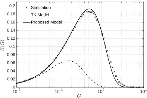
Figure 5. Comparison of simulation results of 1p-CSMA compared to the TK model and to our model fora= 5.
is given by the weighted distribution function of fZ, that is
fZˆ(x) =xfZ(x)/Z¯) [8]; this yields
ˆ
q0=
e−2G 1 + ¯Y
1 + 3 2G
. (21) Substituting (14), (15), (20) and (21) into (13), and the latter into (11), completes the derivation of the model.
V. SIMULATION RESULTS AND MODEL VALIDATION
We simulated the behavior of the system using OM-NeT++ [10]. For the scenario presented in Section II, we set a number of hosts equal to N = 100. The main simulation parameters are a and the average interarrival time for each packet generated by a node, µ = 1
λ = N
G, where G is the
aggregate packet generation rate. New arrivals are generated according to a Poisson process of rateλ. We have run simula-tions for different values ofa: we noticed that the throughput rapidly converges to the same behavior fora≥2. This is due to the fact that the asymptotic behavior of the rates is achieved rapidly asaincreases. The TK model is outperformed by the one introduced here even in the presence of the approximations in (9) and (10), and under our assumptions onPs(G)in (12)
and onξ¯.
Fig. 5 shows S(G) vs. G for 1p-CSMA as obtained by OMNeT++ simulations in the case a = 5, and compares it to the TK model and to our proposed model. We observe that the match between our model and the simulation is very good, whereas the TK model severely underestimated the maximum throughput (about1/3of the value observed in the simulations) and also underestimates the value ofGat which the maximum throughput is achieved.
Finally, Fig. 6 showsS(G)vs.Gfor various values ofa: for values of a ≥2 the simulation curves become progressively harder to distinguish, and are very well approximated by the model. From this result, and from the fact that our model is independent of a, we infer that the influence of the propagation delay onS(G)becomes progressively smaller as
10-2 10-1 100 101 0
0.05 0.1 0.15 0.2
Sim. a = 1 Sim. a = 1.5 Sim. a = 2 Sim. a = 5 Sim. a = 10 Proposed Model TK Model a = 10
a = 1
a = 10
a = 2 a = 1.5
a = 5
G
S
(
G
)
Figure 6. Comparison of simulation results of 1p-CSMA compared to the TK model and to our model.
of transmission successes and collisions at the access point achieves a stationary behavior as a increases, and the only factor that still counts is the normalized packet transmission time, which is identically 1.
VI. CONCLUSIONS
In this paper we have provided an approximate model for 1-persistent (1p) CSMA based on previous observations on non-persistent CSMA in [1]. We highlight that the 1p case is more complex due to the presence of backlogged users, that introduce memory and traffic correlation. However, we show that the evolution of the channel access rate over time has a regular behavior for a≥2, which makes it possible to ap-proximate these rates as constant over time as in the model by Tobagi and Kleinrock (TK). We conclude that the assumptions of the TK model remain valid as an approximation, provided that the expression for the probability of success is modified to account for those transmission successes made possible by the large propagation delays, even in the presence of concurrent accesses.
This fundamental analysis is important for underwater com-munication networks, as in many cases CSMA has been part
of the protocol stack in these scenarios. Our model has been compared against simulations for 1p-CSMA in several cases relevant to underwater networks, showing that it approximates simulations closely for a number of typical values of the propagation delay normalized to the packet transmission time. Future work includes a better characterization of the time period between two subsequent transmission periods, and of the success probability in the presence of concurrent transmis-sions by backlogged users.
ACKNOWLEDGMENTS
This work has been supported in part by the US Office of Naval Research under Grant no. N62909-14-1-N127.
REFERENCES
[1] M. Koseoglu and E. Karasan, “Spatio-temporal analysis of throughput for single-hop CSMA networks,”IEEE Commun. Lett., vol. 18, no. 4, pp. 564–567, Apr. 2014.
[2] C. Petrioli, R. Petroccia, and J. Potter, “Performance evaluation of underwater MAC protocols: From simulation to at-sea testing,” in
Proc. IEEE/OES Oceans, Santander, Spain, Jun. 2011.
[3] K. B. Kredo II and P. Mohapatra, “A hybrid medium access control protocol for underwater wireless networks,” in Proc. ACM WUWNet, Montreal, Canada, Sep. 2007.
[4] Y. Noh, U. Lee, S. Han, P. Wang, D. Torres, J. Kim, and M. Gerla, “DOTS: A propagation delay-aware opportunistic MAC protocol for mobile underwater networks,” IEEE Trans. Mobile Comput., vol. 13, no. 4, pp. 766–782, Apr. 2014.
[5] J. Daladier and M. Labrador, “A data link layer in support of swarm-ing of autonomous underwater vehicles,” in Proc. IEEE/OES Oceans, Bremen, Germany, May 2009.
[6] S. Shahabudeen, M. Motani, and M. Chitre, “Analysis of a high-performance MAC protocol for underwater acoustic networks,” IEEE J. Ocean. Eng., vol. 39, no. 1, pp. 74–89, Jan. 2014.
[7] J. Zhang, X. Ma, G. Qiao, and C. Wang, “A full-duplex based protocol for underwater acoustic communication networks,” inProc. MTS/IEEE Oceans, San Diego, CA, Sep. 2013.
[8] F. Tobagi and L. Kleinrock, “Packet switching in radio channels: Part I–Carrier Sense Multiple-Access modes and their throughput-delay characteristics,”IEEE Trans. Commun., vol. 23, no. 12, pp. 1400–1416, Dec. 1975.
[9] “Evologics underwater SC2R acoustic modem series,” last time accessed: Apr. 2015. [Online]. Available: http://www.evologics.de/en/ products/acoustics/index.html