Mobile Network Resource Optimization
under Imperfect Prediction
Nicola Bui
121
IMDEA Networks Institute, Leganes (Madrid), Spain
2UC3M, Leganes (Madrid), Spain
Abstract—A highly interesting trend in mobile network opti-mization is to exploit knowledge of future network capacity to allow mobile terminals to prefetch data when signal quality is high and to refrain from communication when signal quality is low. While this approach offers remarkable benefits, it relies on the availability of a reliable forecast of system conditions. This paper focuses on the reliability of simple prediction techniques and their impact on resource allocation algorithms. In addition, we propose a resource allocation technique that is robust to prediction uncertainties. The algorithm combines autoregressive filtering and statistical models for short, medium, and long term forecasting. We validate our approach by means of an extensive simulation campaign for different network scenarios. We show that our solution performs close to an omniscient optimizer as well as the simple solution that always maintains a full buffer in terms of prefetching data before it is needed, while at the same time using20% less network resources than the simple full buffer
strategy.
I. INTRODUCTION
“Every form of behavior is compatible with determinism. One dynamic system might fall into a basin of attraction and wind up at a fixed point, whereas another exhibits chaotic behavior indefinitely, but both are completely determinis-tic” [1]. In his provocative essay, Ted Chiang is suggesting that unpredictability is just a consequence of the limitedness of human comprehension. While we do not assume that mobile networks are deterministic, in this paper we take resource optimization in mobile networks one step further by exploiting the predictability of future network capacity.
Mobile networks are increasingly constrained by limited spectral resources, while at the same time user traffic demands are growing steadily [2]. Researchers are addressing this challenge from a variety of perspectives including massive multiple-input multiple-output communications, heterogeneous networks combining femto, micro and macro cells, device-to-device communication, and the concept of exploiting knowl-edge about user behavior and the network itself for perfor-mance optimization.
Recent studies [3] highlight how network dynamics [4] can be understood, predicted and linked to human mobility patterns [5]. This ability to predict user and network behavior allows to optimize resource allocation [6], [7]. As such, it is a highly interesting approach to increase the efficiency of mobile networks and deal with future traffic growth.
In this paper, we propose a resource allocation algorithm for mobile networks that leverages link quality prediction and
prediction reliability. We first design an optimal resource allo-cation algorithm that assumes perfect knowledge of the future, as well as a general user capacity forecasting model for mobile networks. We then combine the two to obtain an iterative algorithm achieving near-optimal performance by taking into account the forecast reliability. While some prior work dealt with prediction-based optimization and uncertainty [8]–[10], our approach is the first to combine multi-scale forecasting with a resource allocation scheme that accounts for imperfect throughput prediction in mobile networks.
The rest of the paper is structured as follows: Section II provides a brief summary of the related work. Section III describes the system model and assumptions. In Section IV we detail the omniscient resource allocation algorithm. Sec-tion V analyzes future predicSec-tion feasibility and its limits: Section V-A gives details about the filtering technique used to obtain short term predictions and Section V-B provides the statistical tools for medium to long term forecasting. Section VI provides our solution for resource allocation under imperfect predictions and the performance of this algorithm is analyzed in Section VII. Section VIII provides our final considerations and next objectives.
II. RELATED WORK
Several recent papers, for example [6] and [7], optimize mobile video delivery by exploiting future knowledge in order to save both energy and cost. The main idea is that it is better to communicate when the signal quality is good and refrain from doing so when the signal quality is bad: better signal quality results in higher spectral efficiency and less resources have to be used to send the same amount of data.
This paper starts from a more general formulation of the problem. We do not limit our approach to video delivery but address data exchange in general. Also, we relax the assump-tion of perfect knowledge of future system condiassump-tions, taking into consideration prediction techniques and their reliability. (Note that in this paper we do not address content prediction and we assume it is known in advance what content the user will be interested in [11].)
Markovian estimators or trajectory-based forecasting tech-niques.
A further key aspect of our paper is the statistic description of the per user capacity in mobile networks. To this end, we modified the models proposed in [4] and [17] to account for imprecise information.
Finally, a number of papers deal with system optimization under imperfect state prediction: [8] studies throughput maxi-mization under imperfect channel knowledge, [10] investigates the impact of imperfect load prediction in cloud comput-ing, and [9] studies resource allocation under uncertainties. However, to the best of our knowledge, our paper is the first attempt combining actual prediction techniques, statistical models, and resource allocation into a practical algorithm for mobile network optimization.
III. SYSTEM MODEL
In this paper we address the downlink from a base station of a mobile network (eNodeB) to a single receiver (UE). To simplify the description of the problem, we consider slotted
time with slot duration t and thus the quantities discussed in
the paper are discrete time series. We use i,j, andkto refer to slot indices. The quantities of interest are:
• Position P = {pi ∈ [0, Pmax], i ∈ N}, where pi is the
distance between UE and eNodeB and Pmax is the coverage
range.
• Active usersN ={ni, i∈N}, where ni is the number of
active users that are in the same cell as the UE. It reflects the congestion level of the cell.
• Signal to interference plus noise ratio (SINR) S = {si ∈
R, i∈N}, wheresi is obtained frompi as follows:
si=s0p−i αfF. (1)
Here,s0is a system constant,αis the path loss exponent and
fF is a random multiplicative term to account for fast fading.
• User cell capacity C ={ci ∈[0, Cmax], i∈N}, where ci
represents the average capacity obtained by the user during slot
i.Cmax is the maximum capacity allocable to the UE, given
the specific mobile technology. We compute ci as a function
ofsi andni through
ci=c0gc(si, ni), (2)
wherec0is a system constant andgcis a technology dependent
function which models system level variables such scheduling policy, congestion, spectral efficiency, etc. In the rest of the paper we consider LTE as the mobile network technology and we adopt the model in [17], which provides a closed form expression forfFandgcfor a user at a given distance from the
base station, when anothern−1users are uniformly distributed in the cell area and proportionally fair scheduling is used. • Receive rate R ={ri ∈ [0, ci], i∈ N}: this is the rate at
which the base station sends data to the UE in sloti.
• Download requirement D = {di ∈ [0, Dmax], i ∈ N},
where Dmax is the maximum data consumption rate of the
most communication intensive application. In slot i, the user
consumesdi bytes of data if they are available. If at any time
the user receives more data than required, the excess can be
stored in a buffer for later use.
• Buffer state B ={bi ∈ [0, BM], i ∈ N}, where bi is the
buffer level andBM is the buffer size in bytes.
• Buffer under-run time U = {ui ∈ [0,1], i ∈ N} is the
fraction of slotifor which no data was available to satisfy the download requirements.
The aforementioned quantities are linked as follows:
bi+1 = min{max{bi+ri−di,0}, BM} (3)
ui =
max{d
i−ri−bi,0}/di di>0
0 di= 0
. (4)
The buffer fills (up to the full buffer BM) whenever the
download rate is higher than the consumption rate,ri> di. In
caseri< di, the algorithm empties the buffer and accumulates
buffer under-run time wheneverbi+ri< di.
In what follows, we refer to function y = gy(x) as gy.
Similarly, we refer to the probability density function and the
cumulative density function (CDF) of a random variableX as
fX(x) and FX(x) =R−∞x fX(y)dy and with µX andσX to
its mean and standard deviation.
IV. RESOURCE ALLOCATION OPTIMIZATION WITH PERFECT FORECAST
The resource allocation problem aims at finding the optimal
rate time series Rthat satisfies the download requirementsD
by using the available capacityC in the best way. We define
the following objective function:
O={oi=ri/ci∈[0,1], i∈N}, (5)
whereoiis the fraction of the available capacity used in sloti
and represents a cost. Note that the same raterhas a different cost oi > oj if the available capacity ci < cj. We obtain the
following optimization problem:
minimize
R
X
i
oi
subject to: X
i
ui=
X
i
u∗i,
bi≤BM, ∀i∈N, (6)
where P
iu∗i is the minimum feasible buffer under-run time.
To minimize this cost function, the base station should send more data when the available capacity is high and use just the minimum rate required to avoid a buffer under-run when the capacity is low.
The solution of Eq. 6 is the optimal resource allocation
strategy R∗ that achieves the minimum buffer under-run time
P
iu∗i at the lowest cost
P
io∗i. If the sequenceC is known
a priori, various offline algorithms can be used to determine the optimal resource allocation. We use a simple water-filling algorithm, which is able to achieve optimality using
the following rules: i) define the break-point el as the last
slot for which all previous rates are finalized (i.e., no more
rate can be used in slots up to el) if either bel = BM or
rk =ck,∀el−1 < k ≤el; ii) define an optimization window
allocated in all slots in el−1< k≤elis finalized;iii) starting
from l= 0,el= 0andm= 1the algorithm accounts for the
slots in the set{el+ 1, . . . , el+m}to satisfy the requirements
up to slot el+m; the algorithm chooses a slot if it has the
highest capacity among the unused ones in the set. iv) the
algorithm either increments l, updatesel and resets m= 0if
a break-point is found or incrementsm. The complete
water-filling algorithm is given in Algorithm 1.sAdd(X, x)adds the element x to the sorted list X in the correct position, π(ci)
gives the position in C of the element ci andshift(D, uj, j)
is a shift function that recomputes the requirements sequence
D accounting for a buffer under-run event uj in slot j. The
following conditions are used:
•I1:=∃el< j≤el+m|bj =BM to verify whether a full
buffer state is reached,
•I2 := Pjel=+elm+1cj −rj = 0 to verify whether all of the
available capacity is used, and
•I3 := Pelj=+eml+1rj −dj = 0 to verify whether all of the
download requirements have been satisfied.
In the following we prove the optimality of Algorithm 1 and discuss the behavior of the algorithm when knowledge of the future capacity is not perfect.
Theorem 1 (Water-Filling Optimality): IfRis a solution of
Algorithm 1 with C and D as inputs and achieves a buffer
under-run time P
iui and cost Pioi, then there exists no
other allocation strategy R′ 6= R for C and D that obtains
performanceP
iu′i and
P
io′i, for which (
P
iu′i<
P
iui)∨
(P
iu′ =
P
iui ∧Pi <
P
ioi), i.e., it has either a lower
buffer under-run time or the same buffer under-run time and a lower cost.
Proof: Theorem 1 can be proven by contradiction on the following hypotheses:
1) P
iu′i<
P
iui
2) ifP
iu′i=
P
iui⇒Pio′i<
P
ioi
For 1)R cannot satisfy the requirementsD in all the slots,
thus P
iu′i <
P
iui ⇒ ∃j s.t. rj +bj < r′j +b′j < dj.
Since R′ 6=R, they must differ before or on slotj in order
to cause the larger under-run time, because any variation later
than that cannot decrease P
iu′i. Since R is obtained using
Algorithm 1 and must result in uj >0, then for all the slots
belonging to the analysis window [el−1+ 1, el], where el =
j the whole available capacity must have been used, which
means R′ cannot use more capacity there to avoid the buffer
under-run.R′cannot use more capacity before slote
l−1either,
since that would impact in a window already completed (ended because of condition I1). Thus, Piu′i ≥
P
iui if the two
strategies are different, which contradicts the first hypothesis. For 2) it is (R6=R′)∧(P
iui=Piu′i)∧(
P
ioi<Pio′i),
thus the two strategies must differ in at least two slots j, k, where cj > ck and (rj < rj′)∧(rk > rk′). The two slots j, k
cannot belong to the same window, because Algorithm 1 uses the slots from a sorted list and finishes either with a full buffer
or when the whole capacity has been used. The two slots j, k
cannot belong to different windows either, because ifj < k, it would have been possible to use more capacity earlier in the allocation which is not possible due to the stopping conditions of the algorithms, whereas ifj > k, a cheaper slot later in the
Algorithm 1 Water-Filling Algorithm (WF)
Input: the knowledge of the future capacity availability C,
the future download requirements D and the initial buffer
levelB0.
Output: R= WF(C, D, B0)
l= 0, el= 0// set the starting point
bel =B0 // set the starting buffer
rel= 0,R=∅// set the starting allocation
while |R|<|D| do
m= 1// set the initial window size
S =∅ // sorted capacity vector initialization
while ¬I1 ∧ ¬I2 ∧ |R|+m <|D|do
S = sAdd(S, cel+m) // add an element to the sorted
capacity list
i= 1
while i≤m ∧ ¬I3 do
rπ(si),old=rπ(si) // store previous allocation rπ(si) = min{rπ(si)+del+m, chi, BM −bπ(si)} //
update the temporary allocation
bπ(si)+j =bπ(si)+j+rπ(si)−rπ(si),old,∀1≤j ≤
m−π(si)
i=i+ 1 end while
m=m+ 1// update the window size
end while if I1 then
l=l+ 1 // increment break-point index
el=j // set last break-point
else
l=l+ 1 // increment break-point index
el=el−1+m// set last break-point
if I2 then
uj= max{dj−rj−bj,0}/dj
D = shift(D, uj, j)// shift D proportionally to uj
starting from slot j
end if end if
R={R, rel−1, . . . , rel}// update the allocation end while
returnR
sequence could have been used instead of a more expensive one earlier in the sequence. However, this is not possible due to either the fact that the more expensive slot must have been used
in order not increaseP
iui(stopping conditionI2) or because
of the ordered selection of the slots (stopping conditionsI1or
I3). Thus,Pio′i ≥
P
ioi if the two strategies are different,
which contradicts the second hypothesis.
Thus, assuming that an allocation strategy R′ provides a
better solution than that obtained using Algorithm 1 violates the hypotheses of the theorem, which is therefore proved.
V. GENERAL FORECAST MODEL
In this section we propose a general model describing the forecasting reliability of a system. In particular, we split our model in three time periods based on the prediction horizon:
Theshort termperiod considers the near future and predicts capacity through time-series filtering techniques [12], [13]. It is characterized by the reliability time τp, which defines how
many slots of the sequence can be predicted and that we will discuss in Section V-A.
The medium term period describes the evolution of the system in terms of available capacity statistics. During this period one or more network cells can be accounted accord-ing to the mobility predictor: Markovian predictors [15] can usually compute the likelihood of visiting a given cell, while trajectory-based predictors [16] provide a more accurate esti-mate by computing the actual distribution of the user position along time.
The long term period provides an overall statistical eval-uation of the available capacity availability based on the steady state distribution of the user position in the network. Both the medium and the long term periods are discussed in Section V-B. Section VI will then provide our resource optimization algorithm.
A. Short term forecast with filters
This section addresses the reliability timeτp achievable by
filtering techniques applied to available capacity time series. In particular, we study autoregressive-moving average (ARMA) filters and their setup according to the system dynamics defined
by the slot timet and the user speedv. We opted for ARMA
instead of GARCH [12], since capacity elements belonging to the short term period are characterized by the same finitte variance.
For each (t ∈[0.5,5], v ∈[0.5,5]) tuple we consider a set
of100capacity traces computed using Eqns. (1,2) as per [17]
starting from the mobility paths of a user moving at constant speed in a random network deployment. We apply the Box-Jenkins [18] method to determine the type and the order of the filter to be used with each sequence. Through the analysis of autocorrelation and partial autocorrelation plots, we find that the best technique for our sequences consists of simple autoregressive (AR) filters of orderτF, and thatτF is inversely
proportional to the tvproduct.
Subsequently, for each of the sequences we estimate filter coefficients by means of the linear least squares procedure [19] and we use the obtained filter to forecast the values of the
other sequences with the same (t, v) parameters. We refer to
a forecast sequence asC˜={c˜i∈[0, Cmax], i∈N}, obtained
from C and to the corresponding error∆ ={δi = ˜ci−ci ∈
[−Cmax, Cmax], i∈N}.
We consider a prediction to be reliable as long as the error
∆ is statistically smaller than estimating the capacity from
its distribution fC(c) or, in other words, when the standard
deviations of the two processes are equal σ∆=σC.
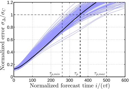
Thus, we compute µ∆ and σ∆ as the average and the
standard deviation of all the error sequences with the same (t, v)parameters. Fig. 1 shows on the abscissa the prediction
0 100 200 300 400 500 600
0 0.2 0.4 0.6 0.8 1 1.2
Normalized forecast timei/(vt)
N
o
rm
a
li
ze
d
er
ro
r
σ∆
/
σC
τp
τp,min τp,max
Fig. 1. The shaded area represents how the standard deviation of the short term prediction error increase with increasing prediction distance varying the user speedvand the slot timet.τprepresents the time after whichσ∆≥σC.
time index normalized on t and on the ordinate σ∆/σC the
standard deviation of the prediction normalized on the standard deviationσC of the original seriesC.
While the actual steepness of the curves varies with the parameters, for all of them the normalized error standard
deviationσ∆/σC approaches1almost linearly. Hence, we set
τp = argminis.t.σ∆i/σC > 1. In addition, we observe that
both τp and the filter order can be approximated with simple
linear models with the inverse of thetvproduct and thatτp is
usually 10times as large as the order of the AR filter. Finally, it is sufficient to tune a set filters for varyingtandv
and select the one to use according to the actual user mobility.
Also, since filters can be normalized on σC it is not needed
to have different filters for different numbers of active users in the cell, but it is sufficient to rescale the constant and the variance parameters of the filter.
B. Statistical models and uncertainties
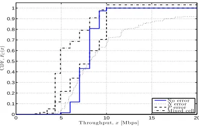
This section describes the second technique of our general forecast model, which adopts statistical models to describe the user capacity availability for medium and long term prediction. In particular, in order to describe the distribution of per user capacity we started again from the model proposed in [17], since to the best of our knowledge it is the only one which takes into account the scheduler impact and thus is able to model user contentions.
In order to account for the impact of uncertainties on the user position and/or the number of active users in the cell we need to modify the expression of the capacity distribution
fC(x)obtained for a specific positionpi and number of users
ni to the actual distribution of the user position fP(x) and
the probability mass function fN(n) of the number of active
0 5 10 15 20 0
0.1 0.2 0.3 0.4 0.5 0.6 0.7 0.8 0.9 1
Throughput,x[Mbps]
C
D
F
,
FC
(
x
)
No error Nerror Perror Mixed cell
Fig. 2. A few examples of the impact of imperfect knowledge on the capacity distribution: the solid line is obtained with accurate information; the dotted and the dashed with imprecision onNandP respectively, while the dash-dotted considers two cells with differentN.
fC(x) =
X
i∈N fN(i)
Z ∞ 0
fF,P|i(gC−1(x, p), p|i)
∂gC−1(x, p)
∂x
dp,
(7)
where fF,P is the joint distribution of fading and position,
gC is the function linking the per user capacity to p and
n and N is the support of fN(n). Since fading and user
position are statistically independent their joint distribution
fF,P(x, y) =fF(x)fP(y)is the product of their distributions.
Eq. (7) modifies the original capacity distribution weighting
it through the active user probability mass function fN(i)
and the user position probabilityfP(y); the partial derivative
normalizes the integrand.
For what concerns our analysis, it is sufficient to be able to compute the per user capacity distribution by accounting for limited knowledge of the user position and traffic in the cell by means of their respective distributions.
So far, our model describes capacity only for the case when the cell the user is connected to is known perfectly. However, to account for different cells it is sufficient to consider the weighted sum of the capacity distributions of single cells
fC,i(x) is the capacity distribution related to cell i and ρi
is the probability of visiting cell iin the next time period, we obtain:
fC(x) =
X
i∈C
ρifC,i(x), (8)
whereC is the set of cells that can be visited in the next time period with some probability.
Fig. 2 provides a few examples of the CDF obtained using the model. The solid line is representative of the capacity CDF
FC(x) when both the active user number n = 5 and the
user position p = 500 meters are exactly known so that the
distribution is equal to the fading distribution. The dotted line accounts for an error on the number of active users in the cell so that fN(x) ={0.2,0.6,0.2}forx={4,5,6}respectively.
Conversely the dashed line is obtained by accounting for an error on the user position which has a normal distribution with
parameters µP = 500 meters and σP = 100meters. Finally,
the dash-dotted line is obtained by mixing together two cells
with 5 and 10users with 20 and80% of visiting probability
respectively. The piecewise-constant shape of the curves is due to discrete relationship between SINR and bitrates.
In a practical implementation of this solution, the capacity statistical models should be known in advance, while the user position statisticfP(x)and the cell traversal timeτ(i)will be
obtained by analyzing user mobility patterns; the number of active users statistic fN(y)in the cell will be estimated from
historic information about that cell at that time of the day. Finally, to define the statistical model for the long term period, we consider a capacity distribution obtained as a mixture of all the capacity distributions of cells in the network weighted through their steady state visiting probability.
VI. RESOURCE ALLOCATION OPTIMIZATION UNDER UNCERTAINTIES
The objective of this section is leveraging the concepts of the previous ones to design a network resource allocation algorithm which takes into account imperfect forecast and that we called Imperfect Capacity prediction-Aware Resource Optimization (ICARO). ICARO aims at minimizing the com-munication cost while avoiding buffer under-runs. In particular, we exploit the water-filling algorithm of Section IV in an iterative way. At each iteration, Algorithm 1 makes a single
decisions about which raterto use by exploiting both the AR
predictor described in Section V-A and the statistical models designed in Section V-B.
Using an iterative algorithm allows to ensures that the optimization algorithm is only making decision about actual capacity values, but taking into account the future evolution of the sequence.
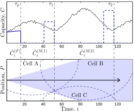
Before describing the new algorithm, we first have to com-bine the aforementioned tools into a single general capacity prediction which can be used with Algorithm 1. In order to account for the three time periods described in Section V we proceed as follows (see Fig. 3):
1) The short term predictionc˜(iF)withi∈[0, τp]is obtained
from the past capacity information collected, for example, by means of lightweight measurements [20] and choosing the filter order τF and coefficients based on the user speedv.
2) The medium term model fC,i(x) is computed as the
superposition of the cellsj ∈ C that the user is likely to visit
in the i-th time period, each of them accounted for according
to their user position fP,j(y) [16] and active user number
fN,j(z)[3], [21] statistics by Eq. (8). Similarly, the duration
of the i-th time period τi−τi−1, is obtained as a weighted
sum of cells traversal time τ(j) related to cell j∈(C).
3) During the i-th time periodDi=Pτij=τi−1dj
bytes has to be downloaded to avoid buffer under-run. The maximum cell efficiency is achieved when only the slots with the highest capacity are used.
4) The highest thresholdcT,iis computed so that the average
amount of data obtained by selecting only the slots with larger a capacity thancT is larger thanDi/(τi−τi−1):
cT,i= max
y s.t.
Z ∞
y
20 40 60 80 100 120
P
o
si
ti
o
n
,
P
Time,i
20 40 60 80 100 120
C
a
p
a
ci
ty
,
C
Cell A Cell B
Cell C ˜
Ci(F) C˜i(M,1) C˜i(M,2)
τp τ1 τ2
Fig. 3. The upper part of the figure illustrates a sequence obtained through our mixed predictor: autoregressive filtering until τp, statistical model until τ2. The lower part shows a possible example of the user movement, where the horizontal arrow is the user direction and the shaded area contains the set of positions where the user can be predicted to be.
5) Thei-th time period is modeled as a sequence ofτi−τi−1
values
˜
c(jM,i)=
c
T,i j >(1−FC,i(cT,i))(τi−τi−1)
0 otherwise , (10)
whereFC,i(cT,i)is the probability of the capacity being lower
thancT,i, thus(1−FC,i(cT,i))(τi−τi−1)is the average number
of slots with larger capacity than the threshold.
6) Steps2to5are repeated and new time periods are added
in the sequence if their reliability is sufficient (two cells, if Markovian predictors are used [15]).
7) Computeτoas the offset time when the user first entered
in the cell.
8) Obtain the predicted capacity sequence as the concatena-tion of the previously computed time period sequences:
˜
ci=
c0 i= 0 ˜
c(iF) 0< i≤τp
˜
c(iM,1) τp< i≤τ1∧τ1> τp+τo
˜
c(iM,2) max(τo+τp, τ1)< i≤τ2
· · · ˜
c(iM,n) τn−1< i≤τn
, (11)
where τn is the duration of the whole sequence, c0 is the
known present capacity,˜c(iM,1)is modified by removing slots from the beginning (˜c(iM,1) = 0) if the past capacity values and those predicted with ˜c(iF) are lower thancT,1 or from the
end (˜c(iM,1)=cT,1) if the opposite is true.
Fig. 3 shows an example of a mixed model sequence: in the upper part, the thin solid line represents the ground
truth available capacity C, the thick solid line is the short
term prediction C˜(F) and the dashed line represents two
cells through their statistics by means of C˜(M,1) andC˜(M,2)
respectively. The lower part of the figure represents a map where the user is moving from the left to the right following the central horizontal solid line. The shaded area highlights the area where the user is likely to be The dashed circles represent the coverage areas of different cells. Finally, dash-dotted lines crossing the two parts of the figures markτp,τ1andτ2instants.
ICARO, which is detailed in the following Algorithm 2, uses the water-filling algorithm to allocate rate iteratively based on the mixed forecast sequence of Eq. (11). The algorithm ends if the total remaining required bytes is smaller or equal than the current buffer level.
Algorithm 2 Imperfect Capacity prediction-Aware Resource Optimization (ICARO)
Input: the future download requirementD, user speedv and
position p, τF past values of the capacity sampled with
t period, the capacity statistics fC,i(x) and time period
traversal timeτi for the next predictable time periods.
Output: R, O, U
s= 0// set the starting point
bs=B0 // set the starting buffer
rs= 0,R=∅ // set the starting allocation
while P|D|
i=sdi≥bs do
computeC˜ as per Eq. (11)
run Rˆ= WF( ˜C, D, bs)
rs= min(ˆr1, cs, BM −bs)// rate to be used
if cs then
os=rs/cs // cost
else
os= 0
end if
if ds>0 then
us= max((ds−bs+rs),0)/ds // buffer under-run
else
us= 0
end if
bs+1 = min(max(bs+rs−ds,0), BM)// next buffer
if us>0then
D= shift(D, us, s)
end if
s=s+ 1
D ={di, s < i≤ |D|} // remove the first element from
the requirements sequence
end while
returnR, O, U
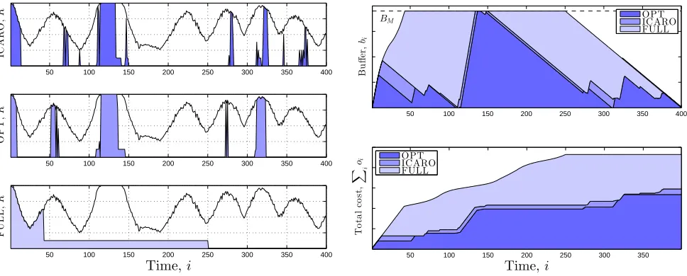
The rationale for using the water-filling algorithm on the mixed forecast sequence is that its operational principle, that selects which slot to use in descending order, still works under uncertainties and provides a solution which is conservative (as the highest capacity slots are placed last) to avoid under-runs, and aggressive (as the allocation priority is given to the most reliable slots) to optimize allocation costs. In the following, we provide a few examples of the algorithm:
50 100 150 200 250 300 350 400
IC
A
R
O
,
R
50 100 150 200 250 300 350 400
O
P
T
,
R
50 100 150 200 250 300 350 400
F
U
L
L
,
R
Time, i
50 100 150 200 250 300 350 400
B
u
ff
er
,
bi
OPT ICARO FULL
50 100 150 200 250 300 350
Time,i
T
o
ta
l
co
st
,
X
i
oi OPTICARO
FULL
BM
Fig. 4. ICARO algorithm output is compared to the optimal allocation (OPT) and the most conservative approach (FULL) on the left. On the right the differences between the buffer state and the cost evolutions of the three algorithms.
order of those of the actual sequence. In fact, as we showed in Section V-A, σδ,i is increasing withi, thus if˜c(iF)>c˜
(F)
j and
j > i, then the same ordering probability is larger than that of opposite order (P[ci > cj] > P[ci ≤ cj]). Thus, the
water-filling algorithm can be used on the short term prediction, because its order is likely to match that of the actual sequence. Ordering between short and medium term forecast: the
i-th medium term period is represented as a sequence of
(τi−τi−1)FC,i(cT,i)zero capacity slots while the remaining
slots are equal to cT,i. Hence, if the short term prediction is
lower than cT,1 only the minimum rate is used, since from
the statistical model slots of higher capacity are expected to come later. Conversely, if the short term prediction is larger thancT,1, then it is more likely that the remaining slots will be
lower than the threshold (compare with step 8 of the sequence creation).
Buffering: the algorithm will always try to use the slots above threshold in each time periods and bridge those by using the buffer. By positioning the slots with highest capacity at the end of each time periods we ensure that the algorithm is
conservative. Finally, the maximum buffer size BM limits the
optimization horizon of the algorithm: in fact, the maximum time that the system can last without using any capacity is given by BM/(Pidi/|D|). Hence, the buffer size has a
significant impact on the algorithm performance which we analyze in the next section.
Fig. 4 shows an example of ICARO’s performance compared to the optimal boundary (OPT) obtained with perfect forecast and to the trivial (FULL) solution which maintains the buffer as full as possible. Fig. 4(a) shows three plots of the used
rate Rof the three algorithm: ICARO in the topmost part, the
OPT in the center and FULL at the bottom. In all three plots the shaded area represents the used part of the total available capacity which is drawn as a solid line.
The main difference among the three solutions is that FULL
continues to fill the buffer during the low quality period at
about i= 25, while OPT just use the needed quantity to be
able to harness the best part of the second cell (i= 50), while ICARO, being more conservative than the optimal solution, accumulates more in the beginning and needs to make some
suboptimal decisions (i.e.: i = 80). In the rest of the trace,
FULL continues downloading just the needed to maintain the buffer full, OPT is able to use the best slots only, while ICARO performs very close to OPT.
Similar considerations can be derived from Fig. 4(a): the upper part shows the buffer variation for the three schemes, while the lower part reports the cumulative cost. We can remark that ICARO performs very close to OPT, but it is always slightly more conservative as the buffer is always a bit fuller earlier on. Also, even though the cost is higher than the optimal, the two algorithms perform quite the same.
VII. RESULTS
In this section we provide an analysis of the overall perfor-mance of our algorithm. Since, to the best of our knowledge no other solution is able to compute resource allocation while accounting for the impact of prediction uncertainties, we com-pare our solution with the optimum offline allocation (OPT) computed with the optimal water-filling algorithm on the exact capacity time series and the most conservative approach (FULL) which just fills up the buffer as soon as possible and maintains it as full as possible until the download requirements are satisfied.
The main performance metrics we are interested in are the
objective functionOand the buffer under-run timeU. In order
to be able to mix the results of every tested configuration,
we adopt the average cost ξ = P
ioi/|O|, the average cost
savingη= (P
ioi,FULL−oi,ICARO)/Pioi,FULLobtained by
our algorithm, and the average buffer under-run time increase
ζ=P
20 40 60 80 100 120 140 160 180 200 0.07 0.08 0.09 0.1 0.11
20 40 60 80 100 120 140 160 180 200 0.4 0.45 0.5 0.55 A v er a g e co st , ξ
20 40 60 80 100 120 140 160 180 200 0.8
0.85 0.9
Normalized buffer size,BMC/D
ICARO OPT FULL
D/C= 0.1
D/C= 0.5
D/C= 0.9
50 100 150 200
0.1 0.2 0.3 0.4 0.5 0.6 0.7 0.8 0.9 0.05 0.05 0.05 0.05 0.05 0.1 0.1 0.1 0.1 0.1 0.15 0.15 0.15 0.15 0.15 0.2 0.2 0.2 0.2 0.25 0.25 0.25
Normalized buffer size,BMC/D
N o rm a li ze d re q u ir em en t, D / C
Cost saving,η
50 100 150 200
0.1 0.2 0.3 0.4 0.5 0.6 0.7 0.8 0.9 0.0001 0.0001 0.0001 0.0001 0.0001 0.0001 0.001 0.001
Normalized buffer size,BMC/D
N o rm a li ze d re q u ir em en t, D / C
Under-run time increase,ζ
Optimal buffer under-runU
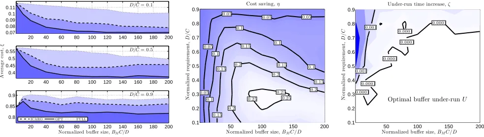
Fig. 5. Overall performance comparison among ICARO, OPT and FULL algorithms in the suburban scenario.ξ,ηandζfor different operational conditions (BMPici/PidiandPidi/Pici) are plotted on the left, center and right respectively.
We analyze two LTE network scenarios: a suburban envi-ronment with users moving at moderate vehicular speed and
a pedestrian urban environment (µv = 5 and 1 meters per
second). Both scenarios have been simulated by generating
random networks of 100adjacent cells with average distance
between base stations of 500 meters and 1.5 kilometers
re-spectively. Results obtained in the two scenarios are shown in Fig. 5 and Fig. 6.
To generate capacity traces we use the Hata model [22] for the path loss, the Rayleigh distribution for the fast fading and we follow the analysis of proportional fair scheduling in [17] to obtain the capacity distribution of a UE at a given distance
from the eNodeB, when there are N active users uniformly
distributed in the cell.
Each simulation group is defined by a network deployment and a reference path which the user follows to cross the net-work. The time it takes to traverse the path is2000t/vseconds.
To train the system we study50other paths following random
trajectories within a cell coverage range from the reference path. We use trajectory based predictors in suburban simulation and Markovian estimators for the urban ones. Subsequently,
we validate the system on 25other paths generated from the
same reference while using the information gathered from the training set for the predictions.
For each tuple (v ∈ [0.5,5], t ∈ [0.5,5]) we generate
20 groups of simulations. Finally, during the validation we
vary the requirement over capacity ratio (P
idi/Pici) ∈
[0.1,0.9], and the normalized buffer size(BMPici/Pidi)∈
[1,200].
Fig. 5 (left) shows the average cost ξ of the three
algo-rithms (OPT, ICARO and FULL as solid, dashed and dash dotted lines, respectively) varying the buffer size (x-axis) for
P
idi/
P
ici={0.1,0.5,0.9}(upper, center and lower plots).
In the upper plot the download requirements are moderate and both OPT and ICARO are able to obtain a normalized cost
lower than0.08(corresponding to80% of theP
idi/Pici),
while FULL needs 95% of the resource (ξ = 0.095). The
performance is coherent in the other plots and ICARO is always better than FULL and close to OPT. As expected, ICARO performance improves when the buffer is larger and the requirements are lower. Notably, when the buffer is very
small the three algorithms perform the same. However, the per-formance degradation for large buffer size has to be ascribed to the simulation length: in fact, in order to fully exploit a large buffer a proportionally longer time is needed.
The central figure shows contour plots of ICARO’s effi-ciencyηusingBMPici/Pidias abscissa andPidi/Pici
as ordinate: the curves are labeled according to the cost savings achieved and the area is colored with a darker shade if the saving is lower. Again the best results are obtained for medium
buffer and small requirements where ICARO is more than25%
cheaper than FULL. On average, ICARO is 8% worse than
OPT.
The figure on the right shows how close is ICARO to the optimal buffer under-run time obtained by both OPT and
FULL. We plot ζ using the same coordinates as those of
the previous figure. Here the white part of figure highlights where ICARO is able to achieve optimal performance, while other darker areas correspond to slightly worse performance. Notably, for no parameters the buffer under-run time was larger than0.01tand very rarely larger than0.001t, chiefly for high
requirement and small buffer size. Also, the 0.0001t contour
is noisy due to the system sensitivity to input parameters in that particular region.
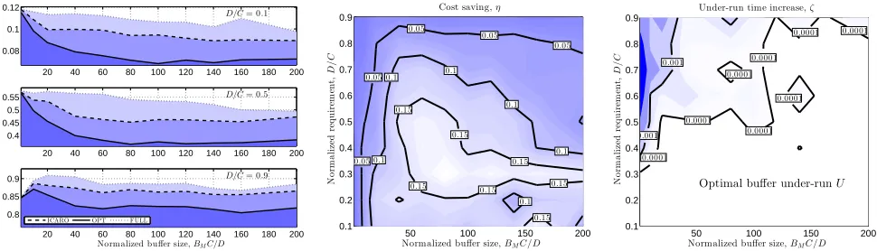
Fig. 6 provides results equivalent to those of the previous set of figures, but obtained for the urban scenario. Here, ICARO performance is slightly worse than those obtained in the suburban scenario. This is due to two main reasons: first, the urban environment shows a lower time correlation due to a more scattered fast fading and, second, to the lower accuracy of Markovian estimation compared to trajectory-based predictors. Nonetheless, ICARO maintains, in the urban scenario, the positive outcome obtained in the suburban: the buffer under-run time (right) is most often optimal and, when it is not,
the increase never reaches 1% of the buffer under-run time
obtained by OPT; the cost savings (center) are mostly larger
than10% and as good as20% in a limited parameter region.
Since ICARO gives priority to avoiding buffer under-runs, it can obtain higher cost savings when the ratio between
requirements and available capacity is lower. Thus, since ζ is
always lower than1%, the algorithm is able to trade off cost
20 40 60 80 100 120 140 160 180 200 0.08
0.1 0.12
20 40 60 80 100 120 140 160 180 200 0.4
0.45 0.5 0.55
A
v
er
a
g
e
co
st
,
ξ
20 40 60 80 100 120 140 160 180 200 0.8
0.85 0.9
Normalized buffer size,BMC/D
ICARO OPT FULL
D/C= 0.1
D/C= 0.5
D/C= 0.9
50 100 150 200
0.1 0.2 0.3 0.4 0.5 0.6 0.7 0.8 0.9
0.05 0.05
0.05
0.05
0.05
0.1
0.1 0.1
0.1
0.1
0.1
0.15 0.15 0.15 0.15
0.15 0.15 0.15
Normalized buffer size,BMC/D
N
o
rm
a
li
ze
d
re
q
u
ir
em
en
t,
D
/
C
Cost saving,η
50 100 150 200
0.1 0.2 0.3 0.4 0.5 0.6 0.7 0.8 0.9
0.0001
0.0001 0.0001
0.0001
0.0001 0.0001
0.0001 0.0001 0.001
0.001
Normalized buffer size,BMC/D
N
o
rm
a
li
ze
d
re
q
u
ir
em
en
t,
D
/
C
Under-run time increase,ζ
Optimal buffer under-runU
Fig. 6. Overall performance comparison among ICARO, OPT and FULL algorithms in the urban scenario.ξ,η andζfor different operational conditions (BMPici/PidiandPidi/Pici) are plotted on the left, center and right respectively.
to 25% cost reduction when the conditions are favorable, but
it is never too aggressive when the future capacity estimation does not allow to do so.
Finally, when ICARO achieves the best results, the system is able to sustain the same quality of service while saving
up 25% of the network resources or, analogously, 25% more
users can be served with the same capacity. Conversely, where it obtains the worst performance, it is the system condition itself that offers small improvement margins: in particular for very small buffer sizes and/or high requirements.
VIII. CONCLUSION
In this paper we addressed the problem of resource opti-mization for mobile networks under imperfect prediction of future available capacity. To this aim we developed a general prediction model that allowed us to account for different prediction tools to encompass short to medium and long term prediction. This joint estimation technique allowed us to design ICARO, a lightweight resource optimization algorithm which achieves close-to-optimal performance. It achieves a nearly optimal buffer under-run time, which never exceeds the optimal
time by more than1%. In addition, ICARO is effective in the
robustness/efficiency trade off. When the system conditions
permit, it saves up to 25% of the network resources.
As a final remark, ICARO is the first practical resource optimization algorithm that does not assume perfect knowl-edge of the future system evolution and thus demonstrate the feasibility of prediction-enhanced optimization techniques for mobile networks.
ACKNOWLEDGMENT
The research leading to these results was partly funded by the European Union under the project eCOUSIN (EU-FP7-318398).
REFERENCES
[1] T. Chiang, “What’s expected of us,” Nature, vol. 436, no. 7047, pp. 150–150, 2005.
[2] S. Wang, Y. Xin, S. Chen, W. Zhang, and C. Wang, “Enhancing spectral efficiency for LTE-advanced and beyond cellular networks [Guest Editorial],”IEEE Wireless Communications, vol. 21, no. 2, pp. 8–9, April 2014.
[3] U. Paul, A. P. Subramanian, M. M. Buddhikot, and S. R. Das, “Understanding traffic dynamics in cellular data networks,” in IEEE
INFOCOM, Shangai, China, April 2011, pp. 882–890.
[4] M. Z. Shafiq, L. Ji, A. X. Liu, and J. Wang, “Characterizing and model-ing internet traffic dynamics of cellular devices,” inACM SIGMETRICS, New York, NY, USA, 2011, pp. 305–316.
[5] M. C. Gonzalez, C. A. Hidalgo, and A.-L. Barabasi, “Understanding individual human mobility patterns,” Nature, vol. 453, no. 7196, pp. 779–782, 2008.
[6] Z. Lu and G. de Veciana, “Optimizing stored video delivery for mobile networks: The value of knowing the future,” inIEEE INFOCOM, Turin, Italy, April 2013, pp. 2706–2714.
[7] H. Abou-zeid, H. Hassanein, and S. Valentin, “Energy-efficient adaptive video transmission: Exploiting rate predictions in wireless networks,”
IEEE Transactions on Vehicular Technology, vol. 63, no. 5, pp. 2013–
2026, June 2014.
[8] J. Rasool and G. Oien, “Maximizing the throughput guarantees in wire-less networks under imperfect channel knowledge,” in IEEE WCNC, Paris, France, April 2012, pp. 2225–2229.
[9] K. Akkarajitsakul, E. Hossain, and D. Niyato, “Distributed resource allocation in wireless networks under uncertainty and application of bayesian game,”IEEE Communications Magazine, vol. 49, no. 8, pp. 120–127, 2011.
[10] F. Jokhio, A. Ashraf, S. Lafond, I. Porres, and J. Lilius, “Prediction-based dynamic resource allocation for video transcoding in cloud computing,” inIEEE PDP, Belfast, Ireland, February 2013, pp. 254– 261.
[11] M. Ahmed, S. Spagna, F. Huici, and S. Niccolini, “A peek into the future: predicting the evolution of popularity in user generated content,”
inACM WSDM, Rome, Italy, February 2013, pp. 607–616.
[12] N. Sadek and A. Khotanzad, “Multi-scale high-speed network traffic prediction using k-factor gegenbauer arma model,” inIEEE ICC, vol. 4, Paris, France, June 2004, pp. 2148–2152.
[13] Y. Qiao, J. Skicewicz, and P. Dinda, “An empirical study of the multiscale predictability of network traffic,” inIEEE HDPC, Honolulu, Hawaii USA, June 2004, pp. 66–76.
[14] N. Bui, F. Michelinakis, and J. Widmer, “A model for throughput prediction for mobile users,” inEuropean Wireless, Barcelona, Spain, May 2014.
[16] J. Froehlich and J. Krumm, “Route prediction from trip observations,”
SAE SP, vol. 2193, p. 53, 2008.
[17] O. Østerbø, “Scheduling and capacity estimation in lte,” inIEEE ITC, San Francisco, CA, USA, September 2011, pp. 63–70.
[18] S. Makridakis and M. Hibon, “ARMA Models and the Box-Jenkins Methodology,” Journal of Forecasting, vol. 16, no. 3, pp. 147–163, 1997.
[19] J. D. Hamilton, Time series analysis. Princeton university press Princeton, 1994, vol. 2.
[20] C. Dovrolis, P. Ramanathan, and D. Moore, “Packet-dispersion
tech-niques and a capacity-estimation methodology,” IEEE/ACM
Transac-tions on Networking, vol. 12, no. 6, pp. 963–977, December 2004.
[21] A. Burulitisz, S. Imre, and S. Szab´o, “On the accuracy of mobility modelling in wireless networks,” inIEEE ICC, vol. 4, Paris, France, June 2004, pp. 2302–2306.