The evolution of internal damage identified by means
of X-ray computed tomography in two steels and the
ensuing relation with Gurson’s numerical modelling
Fernando Suárez1 , Federico Sket2, Jaime C. Gálvez3*, David A. Cendón4, José M. Atienza4 and Jon Molina-Aldareguia2
1 Departamento de Ingeniería Mecánica y Minera, Universidad de Jaén, 23071 Jaén, Spain; [email protected]
2 Instituto IMDEA Materiales, C/ Eric Kandel 2, Tecnogetafe 28906 Madrid, Spain; [email protected];
3 Departamento de Ingeniería Civil-Construcción, Universidad Politécnica de Madrid, E.T.S.I. Caminos,
Canales y Puertos, 28040 Madrid, Spain; [email protected]
4 Departamento de Ciencia de Materiales, Universidad Politécnica de Madrid, E.T.S.I. Caminos, Canales y
Puertos, 28040 Madrid, Spain; [email protected]; [email protected] * Correspondence: [email protected]; Tel.: +034-913-365-350
Abstract:This paper analyses the evolution of the internal damage in two types of steel that show different fracture behaviours, with one of them being the initial material used for manufacturing prestressing steel wires, which shows a flat fracture surface perpendicular to the loading direction, and the other one being a standard steel used in reinforced concrete structures, which shows the typical cup-cone surface. 3mm-diameter cylindrical specimens are tested with a tensile test carried out in several loading stages and, after each of them, unloaded and analysed with X-ray tomography, which allows detection of internal damage throughout the tensile test. In the steel used for reinforcement, damage is developed progressively in the whole specimen, as predicted by Gurson-type models, while in the steel used for manufacturing prestressing steel-wire damage is developed only in the very last part of the test. In addition to the experimental study, a numerical analysis is carried out by means of the finite element method by using a Gurson model to reproduce the material behaviour.
Keywords:Steel, Tensile Test, XRCT, Damage Evolution, Gurson Model
1. Introduction
Steel is, with concrete, the most important building material used at the time, and the standard tensile test is the most widely used method to determine its principal material properties [1]. With it, the stress-strain curve of the material may be obtained before the ultimate tensile strength is reached; stresses and strains are then difficult to estimate. This is why the material behaviour after the ultimate tensile strength is usually neglected. Nevertheless, understanding the fracture mechanisms that lead to the eventual failure is of significant interest, since it can help to improve structural safety strategies.
The fracture of ductile materials has usually been explained with the theory of nucleation, growth and coalescence of microvoids [2]. According to this theory, at a first stage and with high loading being applied, microvoids are developed inside the material (nucleation) due to a decohesive process of small inclusions that are torn apart from the rest of the material or by the fracture of the particle that constitutes the inclusion itself. At a second stage, and under higher strain states, these microvoids increase their size (growth) until they become interconnected (coalescence). Such a process weakens the material until its eventual failure.
This theory has given rise to many mathemathical models, with a special mention to Gurson-type models [3]. Since its appearance, the Gurson model has been applied to reproduce damage evolution in different ductile materials, such as aluminium, copper and steel [4–6]. Subsequent evolution of the model have been able to reproduce not only softening due to the growth of microvoids, but also the
eventual fracture of the material [7]. When such a model is applied to reproduce a tensile test on a ductile material, the damage begins to develop in very early stages of the test, as shown in Figure1.
0.00 0.05 0.10 0.15 0.20
εeng 0
1 2 3 4 5 6 7 8 9
F
[kN]
Gurson model applied No Gurson model applied
Figure 1.F-εcurves obtained with numerical simulations of the same specimen. One of them using a Gurson model and the other one without it.
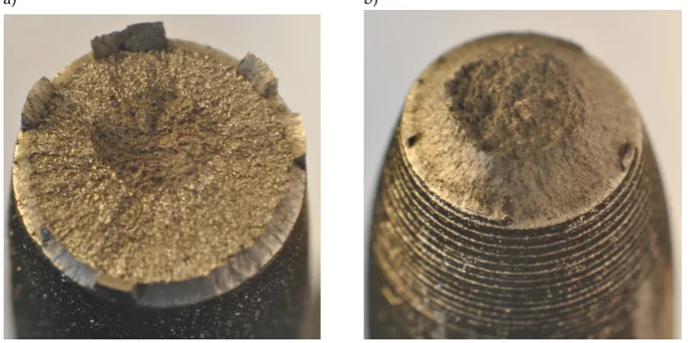
Steel properties may differ depending on many factors, such as the chemical composition and the manufacturing process used. Such differences may affect ductility and the fracture mechanisms that lead to failure, with geometrically identical cylindrical specimens of different steels presenting a contrasting fracture surface after a tensile test. Figure2shows the fracture surface of two 9mm-diameter specimens made of different steels. The one on the left shows a typical cup-cone fracture, usually observed on ductile materials [2] and which belongs to a specimen made of standard steel used in reinforced concrete structures. The one on the right shows a flat fracture surface, where a dark circular region can be observed, belonging to to a specimen made of steel used for manufacturing prestressing steel wires.
a) b)
Figure 2.Fracture surfaces on 9mm-diameter specimens of two steels with different fracture patterns after testing under tension: a) Material 1; b) Material 2 [8].
2b). These materials have been analysed in the past and their mechanical properties are well known; for further information, the reader is referred to [8] and [9]. In the first place, the fracture surfaces of both materials are observed with a scanning electronic microscope to identify the fracture mechanisms that take place. In the second place, an analysis of damage evolution along a tensile test on cylindrical steel specimens is carried out; this analysis is performed for both materials. Specimens are tested in subsequent loading stages and, at the end of each stage, analysed with X-ray computed tomography (XRCT) in order to identify the evolution of the internal damage. Maire et al. ([10–12]) have used a similar approach on aluminium and steel specimens to quantify damage evolution and study the effect of distinct triaxiality states on this process, which has served to compare experimental values of void growth and damage evolution with those predicted by numerical models.
In order to study how one of the most extended numerical models used with metals, the Gurson model, reproduces damage evolution, both tests are numerically reproduced. This numerical study is carried out using the finite element method and the material behaviour is reproduced by the Gurson model. The model is calibrated by using macroscopic results obtained experimentally: the load-strain curve and the necking radius evolution. The evolution of the internal porosity numerically obtained is compared with the experimental values provided by XRCT.
2. Experimental work
2.1. Materials
Two different steels are considered in this work. This section describes their characteristics.
2.1.1. Material 1
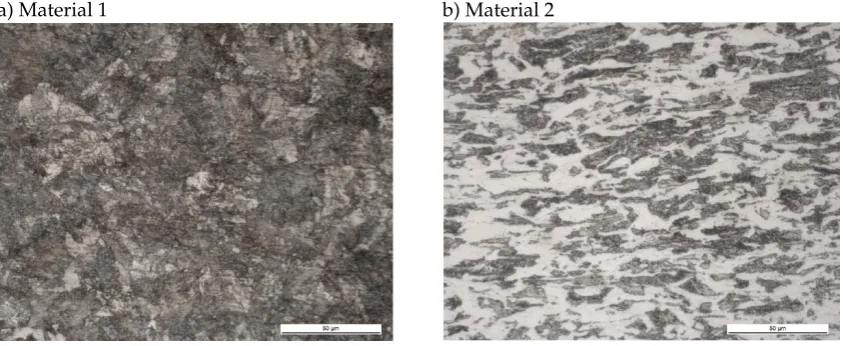
In the manufacturing process to obtain steel wires, raw eutectoid steel bars are cold-drawn, reducing their section by pulling them through a conical die. This process affects the failure behaviour of the material [13,14] and may introduce additional uncertainties in this study. Therefore, for this research, specimens of Material 1 were obtained from raw eutectoid pearlitic steel bars used for manufacturing prestressing steel wires. That is to say, they had not been affected by cold-drawing so the material was as isotropic as possible. The chemical composition of this material can be consulted in Table1. According to the metallographic analysis, the microstructure of this material is formed by perlite, with a lamellar structure of equi-axed grains with an average size of G=9. This microstructure can be seen in Figure3a.
Table 1.Chemical composition of both materials in %.
Material C Si Mn P S Cr Mo
1 0.83 0.25 0.72 0.012 0.004 0.24 <0.01 2 0.22 0.18 1.00 0.024 0.042 0.08 0.03
Material Ni Cu Al Ti Nb V N
1 0.02 0.01 <0.003 <0.005 <0.005 <0.01 0.0097 2 0.14 0.46 <0.003 <0.005 <0.005 <0.01 0.0113
2.1.2. Material 2
a) Material 1 b) Material 2
Figure 3.Microstructure of both materials in the longitudinal direction before testing.
2.2. Specimens
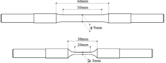
Two diameters were considered for each material: 3mm and 9mm. The 9mm-diameter specimens were used to analyse the fracture surfaces, since comparison is easier in specimens with larger cross sections. The 3mm-diameter specimens were used in the damage evolution analysis to ensure a correct penetration of the X-rays used to identify the internal damage. The dimensions of these specimens can be checked in Figure4.
Figure 4.Specimens dimensions.
2.3. Testing procedure used to study the damage evolution
In order to follow the damage evolution inside a specimen, it was tested in subsequent load stages, after each of which the specimen was unloaded and its neck analysed with X-ray computed tomography (Nanotom 160NF, Phoenix). The steps given for each analysis are given as follows:
1. X-ray tomographic analysis before the specimen is tested.
2. Specimen is tested until the maximum load is reached; then, it is unloaded. 3. X-ray tomographic analysis after the first stage.
4. Specimen is tested until the second stage is reached; then, it is unloaded. 5. X-ray tomographic analysis after the second stage.
6. The previous steps are followed until the point of failure.
a) General view:
b) Detail of the central region (1): c) Detail of the external region (2):
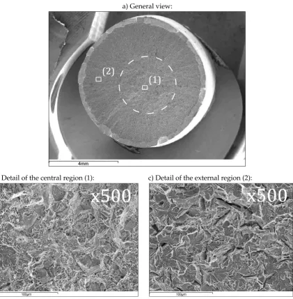
Figure 5.Fractographs obtained from the 9mm-diameter specimen made of Material 1.
2.4. Results
2.4.1. Fractographic analysis of the fracture surfaces
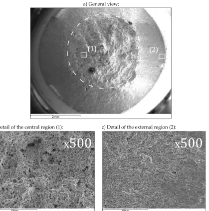
Figure5and Figure6show the fractographs obtained with the 9mm-diameter specimens tested, with the former corresponding to the Material 1 specimen and the latter to the Material 2 specimen. For each of them, a general fractograph of the fracture surface and two closer fractographs are shown, one of the central region of the surface and the other of the external region. The internal region is highlighted by a dotted circumference. In the Material 1 specimen it corresponds to the internal dark region observed after a tensile test and in the Material 2 it corresponds to the flat surface perpendicular to the specimen axis in a cup-cone fracture surface.
a) General view:
b) Detail of the central region (1): c) Detail of the external region (2):
a) Material 1 b) Material 2
Figure 7.Microstructure of both materials in the longitudinal direction after testing.
slightly sharp edges, which seems to indicate a combination of the nucleation, growth and coalescence mechanism with the cleavage mechanism.
2.4.2. Metallographic analysis after the test
Figure7shows the microstructure in the longitudinal direction of Material 1 and Material 2 after the test in the necking region.
In the case of Material 1, raw eutectoid pearlitic steel, no differences can be observed when compared with the microstructure before testing (see Figure3a). In the case of Material 2, standard steel used as reinforcement in concrete structures, grains are oriented in the longitudinal direction after the test and show a shape factor of fsh =4.
2.4.3. Internal damage evolution analysis
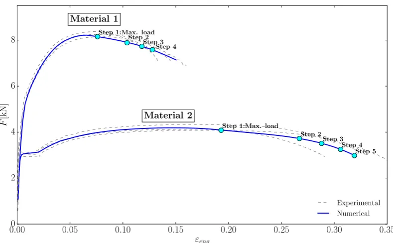
This analysis was performed with 3mm-diameter specimens to allow penetration of X-rays into the material. Since XRCT is an expensive technique that requires much postprocessing work, only one specimen for each material is analysed, which is usual practice when this technique is applied [16–18]. The analysis was carried out with a voxel size of 2.5µm(Nanotom 160 NF, from Phoenix X-ray). As mentioned before, to carry out this analysis the tensile tests were performed in subsequent load stages. These stages are defined by the engineering strain developed along an initial length of 12.5mm and can be consulted in Table2. Figure8shows them over the corresponding F-εengcurves. Note that this figure shows the experimental results for both analysed materials compared with the numerical results that will be described later.
Table 2. Stages used for the damage evolution analysis with the specimens of both materials. Engineering strain over a 12.5mm initial length is used for identifying every stage.
Stage 1 2 3 4 5
Material 1 0.076 0.104 0.118 0.128 — Material 2 0.193 0.267 0.288 0.306 0.319
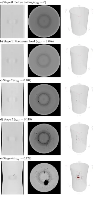
Figure9presents the results for the Material 1 specimen. Results are given for the specimen before testing and for each of the four stages considered. Three pictures are shown for each stage: a longitudinal section of the necking region, a projection of damage on the cross section and a perspective of the internal damage in the necking region.
0.00 0.05 0.10 0.15 0.20 0.25 0.30 0.35 εeng
0 2 4 6 8
F
[kN]
Step 1:Max. load Step 2
Step 3 Step 4
Step 1:Max. load
Step 2 Step 3
Step 4 Step 5
Material 1
Material 2
Experimental Numerical
Figure 8.Load-strain curve of the 3mm-diameter specimen of both materials; comparison between the experimental results and the numerical models. The stages used for the damage evolution analysis are represented with blue circles (the engineering strain has been obtained using an initial gauge length of 12.5 mm).
and coalescence of microvoids, as the test progresses the microvoids start to appear and grow in an even manner but the internal damage that leads the specimen to failure only appears at the very end of the test.
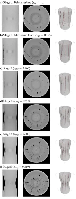
Figure10shows the results for the Material 2 specimen. As in the Material 1 specimen, results are given for before testing and for each of the stages considered, five in this case; and, as in Figure9, three pictures are shown for each of them: a longitudinal section of the necking region, a projection of damage on the floor plan and a perspective of the internal damage in the necking region.
As in the Material 1 specimen, the mechanism of nucleation and growth of voids is clearly noticeable: as the test progresses, evenly spaced voids start to appear and grow.
2.4.4. Longitudinal and radial distribution of voids at each stage
In order to understand how voids nucleate and grow inside the specimen during the test, their distribution has been obtained in the longitudinal direction and in the radial direction for each stage. In the longitudinal direction, the specimen part considered was 3.5mm long centered at the necking area and the void volume was measured for 0.025mm-long slices. In the radial direction the volume was measured at seven concentric hollow cylinders (except the smaller one, which was a full cylinder) of the same volume; this measurement was obtained for 349 slices, 0.8725mm in length. To do this work, the raw data obtained with XRCT was filtered by means of MatlabR scripts and functions [19].
2.5. Discussion on the experimental data
a) Stage 0: Before testing (εeng =0)
b) Stage 1: Maximum load (εeng =0.076)
c) Stage 2 (εeng=0.104)
d) Stage 3 (εeng=0.118)
e) Stage 4 (εeng =0.128)
a) Stage 0: Before testing (εeng =0)
b) Stage 1: Maximum load (εeng =0.193)
c) Stage 2 (εeng=0.267)
d) Stage 3 (εeng=0.288)
e) Stage 4 (εeng =0.306)
f) Stage 5 (εeng=0.319)
Therefore, while the fracture surface of Material 2 and its cup-cone shape agrees with the observations by Bluhm and Morrissey [21] and suggests a clearly ductile behaviour along the test, the fracture surface of Material 1 shows a different fracture behaviour. It suggests that the internal damage, represented by the internal region, develops progressively and opens an internal crack until it eventually fails, propagating the internal crack outwards by a cleavage mechanism. Hence, Material 1 failure presents a brittle-ductile transition phenomenon.
As regards the tomographic images, the initial image obtained for both specimens, before testing, highlights the different nature of both materials. Material 1 has almost no internal voids, whereas Material 2 presents a high volume of them. It is interesting to observe how these voids are lined up longitudinally, which may be due to the manufacturing process.
The different nature of both materials can also be noticed looking at how differently they behave, not only in terms of stress but also in terms of strain; Material 1 has a maximum strain of around 0.13 at failure while Material 2 reaches a value of about 0.34. This is also evident given that necking is much more noticeable in Material 2 than in Material 1.
In Material 1, some small voids can be noticed under maximum loading. As strain increases, new voids appear, some in a random manner but others aligned in the loading direction. The most remarkable observation in this material entails the last stage, an instant very close to failure. Before this instant, voids appear somehow independently and not connected to each other, but at step four some internal cracks seem to have formed, especially a large one in the center of the necking region, generating a large plane crack. This observation agrees with the hypothesis posed in [8,9,22], suggesting that fracture is initiated by an internal crack that, once it reaches a certain size, acts as an internal notch that triggers a brittle fracture process. This is interesting since it allows the use of certain models from the field of linear elastic fracture mechanics which work reasonably well for a clearly elastic-plastic material.
In the case of Material 2, a high number of voids or inclusions is present before any load is applied. As load increases, the voids increase in number and volume. Different from Material 1, no void coalescence can be identified. It is unclear if this means that coalescence takes place just instants before failure or if the test could not be stopped close enough to failure, so internal fracture surfaces could be observed. According to the results reported by Bluhm and Morrisey [21], a fracture plane perpendicular to the loading direction could be expected, which would result in the flat surface of the cup-cone fracture pattern, and finally inclined fracture planes, which would result in the shear planes of the cup-cone shape.
Therefore, the internal damage evolution analysis confirms that, in the case of Material 2, failure is due to a generalised weakening process that takes place all over the cross section as a result of a nucleation, growth and coalescence of microvoids mechanism. In the case of Material 1, although this mechanism is also observed, the eventual failure of the specimen is provoked by an internal crack opening that takes place in the very late instant of the tensile test. This observation confirms that the failure of Material 1 presents a brittle-ductile transition phenomenon where the specimen shows a ductile behaviour until the internal crack is large enough to provoke an eventual brittle failure.
3. Numerical work
3.1. Description of the finite element model
3.1.1. Geometry
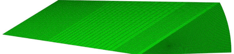
Because of the axial symmetry of the problem, only 1/24th of each specimen has been considered, as shown in Figure11. In order to force necking at thex = 0 plane, the specimen is not perfectly cylindrical, but its radius varies from 1.5mm atx=0 to 1.51mm atx =7.25mm, enough to induce stress concentration numerically atx=0. The mesh was defined after a mesh-size convergence study [22] and resulted in a mesh of 141378 elements shown in Figure12. The length of the elements in the longitudinal direction in the necking region of the specimen was 0.094 mm.
Plane 2
Plane 4
Plane 1 Plane 3
x z
y
Figure 11.Description of the model. Plane 3 represents the eventual plane of failure; displacement is imposed in direction of thexaxis on plane 4.
Figure 12.Mesh used to reproduce the experimental results.
3.1.2. Boundary conditions and load
The load is applied in the X-axis direction and the YZ plane represents the eventual plane of fracture. With regard to the boundary conditions, nodes on thex=0 plane are constrained in thex direction, nodes on thexzplane (plane 1) are constrained only in theydirection and nodes on the inclined plane (plane 2) are constrained only perpendicularly to the plane.
The load is applied by defining an imposed displacement in thexdirection to the nodes placed at x=7.25mm (plane 4).
3.1.3. Materials
The specimens are modelled with a porous elastic-plastic material that follows the Gurson’s formulation available in AbaqusR.
and must be estimated. This has been done by using a parameterrwhich provides the slope after maximum loading asr= ∆σ
∆ε.
However, the porous feature is modelled by a Gurson model, where the yield criterion is given by the expression (1).
Φ=
q
σy
2
+2fcosh
−3p
2σy
−1+f2=0 (1)
wherepandqare the hydrostatic pressure and the von Mises equivalent stress, respectively andf is the void volume fraction.
3.2. Calibrated models
With the aforementioned description of the model, the following parameters can be identified for calibration:
• Material relative density,d. Please, note that here we follow the Gurson model parameters used in the implementation of the model available in AbaqusR, therefore a value ofd=1 implies a fully dense material with an initial void volume fraction of f =0.
• Hardening slope after the maximum load defined as a stress-strain ratio,r. • Mean equivalent plastic strain for void nucleation,εN.
• Standard deviation of the distribution,sN. • Volumetric fraction of nucleated voids, fN.
In order to calibrate both models, the numerical results are compared with the experimental data by means of two criteria. The load-strain curve must be similar enough and the evolution of the necking radius in the center of the neck must follow the same pattern as experimentally observed. Figures8and13show that both criteria are met for both models.
0.00 0.02 0.04 0.06 0.08 0.10 0.12 0.14
εeng
0.0
0.5
1.0
1.5
2.0
nec king radius [mm] Material 1 Experimental Numerical
0.00 0.05 0.10 0.15 0.20 0.25 0.30
εeng
0.0
0.5
1.0
1.5
2.0
nec king radius [mm] Material 2 Experimental Numerical
Figure 13. Necking radius evolution for both materials; numerical and experimental results are compared.
Table 3.Initial parameters for FEM models of both materials.
Material E [N/mm2] ν r d εN sN fN 1 160385 0.30 782 0.999 0.4 0.1 0.02 2 191536 0.30 762 0.99 0.3 0.1 0.06
3.2.1. Comparison with the experimental data
The calibration of both models ensures good agreement with the experimental data at the macroscopic level. Nevertheless, the interest in this study is to compare the evolution of porosity inside the material along the tensile test.
The XRCT technique provides information of the interior of the specimen in the form of voxels grouped in slices. That is to say, a slice is the group of voxels placed at the same longitudinal distance from the fracture plane, considered as the origin. To obtain the void volume fraction (VVF) longitudinal profiles with the experimental data, the porosity fraction is counted for each slice.
Regarding the VVF radial profiles, the void fraction is obtained for concentric cylindrical rings. The inner cylinder is full and the rest are hollow. Throughout this process, the measurement of internal porosity is carefully obtained, neglecting the internal fracture at step four in Material 1 and the longitudinal porosity chains in Material 2, which appear even in the initial tomography, taken before any load is applied.
The same procedure is followed to obtain the VVF longitudinal and radial profiles with the numerical models; to do this, the results obtained with AbaqusR are filtered by several Python-language scripts using NumPy and SciPy libraries [24–26] and the profiles are extracted for the same strain rates considered experimentally (see Table2).
Figure14and Figure15compare the numerical and experimental profiles.
0.0 0.2 0.4 0.6 0.8 1.0 1.2 1.4
r[mm] 0.00
0.01 0.02 0.03 0.04 0.05 0.06 0.07
VVF
−1.5 −1.0 −0.5 0.0 0.5 1.0 1.5
x[mm] 0.00
0.01 0.02 0.03 0.04 0.05 0.06
VVF
Step 1 Step 2 Step 3 Step 4
Figure 14. Radial and longitudinal voids distribution experimentally (continuous lines) and numerically (dashed lines) obtained for Material 1.
In both materials the longitudinal and radial profiles numerically obtained are somewhat different from the experimental ones.
0.0 0.2 0.4 0.6 0.8 1.0 1.2 1.4
r[mm] 0.00
0.05 0.10 0.15 0.20 0.25 0.30 0.35
VVF
−1.5 −1.0 −0.5 0.0 0.5 1.0 1.5
x[mm] 0.00
0.05 0.10 0.15 0.20 0.25
VVF
Step 1 Step 2 Step 3 Step 4 Step 5
Figure 15. Radial and longitudinal voids distribution experimentally (continuous lines) and numerically (dashed lines) obtained for Material 2.
obtained profiles tend to be almost flat, even presenting a higher porosity in the external part of the specimen than that measured experimentally.
In the case of Material 2, both radial and longitudinal profiles may seem to be more similar to the experimental ones, since the porosity profiles for the last step are more similar than in the case of Material 1. Nevertheless, by taking a closer look at these profiles the same differences can be pointed out. In the case of the longitudinal profiles, although the last step profile may seem more or less similar to the experimental one, its evolution is different. For example, while the experimental profile does not develop much in the first two steps and only increases slightly in the steps three and four, the numerical profile develops much from the very first step. Again, as observed for Material 1, the high porosity increment observed experimentally in the last step is not obtained numerically. In the case of the radial profiles, the same differences observed for Material 1 can be identified, since all the numerical profiles are almost flat, different from the numerical ones, and there is not a high porosity evolution in the last step, as experimentally obtained.
From these results, it can be concluded that although a set of parameters provides a macroscopically correct response of the specimen, porosity evolution is different not only for Material 1, which could be expected since it is a steel with a little ductile response and a fracture pattern different from the cup-cone shape, but also for Material 2, which in principle is a material with a behaviour typically reproduced by Gurson-type models.
Nevertheless, it should be noted that in this work the original Gurson model has been used, thus it only reproduces the effects of nucleation and growth of voids, but not coalescence.
3.2.2. Mesh size effect on the voids volume profiles
Mesh density may have a strong influence on the numerical results, that is why, as already mentioned, the model has been calibrated using the using the load-strain curve and the necking evolution. However, there is still no data about how refining the mesh affects the evolution of volume profiles. To this respect, since the mesh is already pretty fine in the radial and angular directions as can be observed in Figure12, with sides of around 20µmin length, only the longitudinal dimension of the elements has been taken into account.
For this study, several meshes have been generated using the same radial and angular discretization and using different element longitudinal lengths in the necking regionl, ranging from a coarse mesh withl=0.75mm. (Figure16a)) to a fine mesh ofl=0.075mm. (Figure Figure16b)).
a) b)
Figure 16.a) Coarser mesh withl=0.75mm. and b) Finer mesh withl=0.075mm..
article, the reader can find all the voids diagrams for each mesh and for all the strain rates considered in this study.
0.0 0.2 0.4 0.6 0.8 1.0 1.2 1.4
r[mm] 0.000
0.002 0.004 0.006 0.008 0.010 0.012 0.014
VVF
l = 0.075 mm. l = 0.094 mm. l = 0.188 mm. l = 0.375 mm. l = 0.750 mm.
0.0 0.2 0.4 0.6 0.8 1.0 1.2 1.4
x[mm] 0.000
0.002 0.004 0.006 0.008 0.010 0.012
VVF
l = 0.075 mm. l = 0.094 mm. l = 0.188 mm. l = 0.375 mm. l = 0.750 mm.
Figure 17.Radial and longitudinal voids distribution of a specimen of Material 1 at step 4 obtained using meshes with different element longitudinal lengths.
In both materials, mesh refinement leads to steeper shapes of both voids distribution, radial and longitudinal. Nevertheless, while in the case of Material 1 the second finer mesh (l=0.094mm.) seems to be fine enough (both diagrams are almost coincident with the finer mesh), in the case of Material 2, it seems that further refinement could lead to slightly steeper shapes of the diagram. This is interesting, since different calibration parameters of the Gurson model seem to require different mesh refinement when the voids distribution shapes are to be analysed.
4. Conclusions
In this paper, two steels with distinct fracture patterns have been analysed, with Material 1 corresponding to an eutectoid steel used for manufacturing prestressing steel wires and Material 2 being a standard steel used as reinforcement in concrete structures. The study has been carried out on 3 mm-diameter cylindrical specimens, tested under tension in subsequent incremental strain steps up to failure. The internal damage evolution has been identified by means of XRCT.
When a specimen of Material 1 is tested, the fracture surface is plane and perpendicular to the loading direction with two different regions: a central dark region and a brighter surrounding region. In the case of a specimen of Material 2, the fracture pattern corresponds to the cup-cone surface, extensively studied by many researchers.
0.0 0.2 0.4 0.6 0.8 1.0 1.2 1.4
r[mm] 0.00
0.05 0.10 0.15 0.20 0.25 0.30
VVF
l = 0.075 mm. l = 0.094 mm. l = 0.188 mm. l = 0.375 mm. l = 0.750 mm.
0.0 0.2 0.4 0.6 0.8 1.0 1.2 1.4
x[mm] 0.00
0.05 0.10 0.15 0.20 0.25
VVF
l = 0.075 mm. l = 0.094 mm. l = 0.188 mm. l = 0.375 mm. l = 0.750 mm.
Figure 18.Radial and longitudinal voids distribution of a specimen of Material 2 at step 5 obtained using meshes with different element longitudinal lengths.
ductile-fragile transition phenomenon. As the test progresses, a ductile behaviour is observed where the nucleation and growth of microvoids mechanism is developed and, immediately before failure, a large penny-shaped internal crack, perpendicular to the loading direction, is formed. This leads to an eventual brittle fracture acting as an internal notch, which agrees well with previous works ([8,9]). Material 2 has an initial high volume of voids or inclusions, probably due to the manufacturing process, which increases as the tensile test is carried out. In this case the fracture is evenly developed over the whole cross section: the nucleation and growth of microvoids mechanism takes place evenly throughout the test and causes a progressive weakening of the material that does not provoke a critical internal crack. Although no internal fracture planes have been observed in Material 2, according to the observations by Bluhm and Morrisey in [21], the progressive formation of the cup-cone fracture surface should be expected. This could be due to a fast formation of this surface before fracture.
Since the Gurson model allows identification of the development of voids inside the material, the test has been numerically reproduced by means of finite element models by using a Gurson porous material. To calibrate the parameters for each material, two macroscopic values have been considered: the load-strain curve and the evolution of the necking radius. After calibration, internal porosity evolution has been compared with that obtained experimentally for both materials in the longitudinal and radial directions.
It is interesting to observe that, although the Gurson model is able to correctly reproduce the two macroscopic criteria used for calibration in both materials, internal porosity profiles differ considerably from the experimental ones. It is also interesting to observe that, when the void volume evolution is analysed, the numerical model calibration may require different mesh refinement for distinct set of calibrated parameters.
The use of a complete Gurson-Tvergaard-Needleman model [7], which includes additional material parameters to account for the effects of void interactions and consider the effect of void coalescence, could help to improve the comparison with the experimental results.
Author Contributions: Jaime C. Gálvez, José M. Atienza and David. A. Cendón conceived and designed the experimental work and supervised the numerical work; Fernando Suárez carried out the experimental work on the tensile testing; Fernando Suárez carried out the the numerical work that deals with the Gurson modelling under the supervision of David A. Cendón; Federico Sket and Jon Molina-Aldareguia carried out the XRCT analysis; Fernando Suárez wrote the paper.
Funding:This research was funded by the Spanish Ministry of Economy, Industry and Competitiveness by means of the Research Fund Project BIA 2016 78742-C2-2-R.
Conflicts of Interest:The authors declare no conflict of interest. The funding sponsors had no role in the design of the study; in the collection, analysis or interpretation of data; in the writing of the manuscript and in the decision to publish the results.
Appendix A. Voids Volume evolution profiles
In order to give a glimpse on how radial and longitudinal voids evolution profiles are affected by the longitudinal size of the elements in the numerical model, this appendix shows them for each of the strain stages experimentally analysed using different longitudinal element lengthsl, ranging from 0.75 mm. to 0.075 mm.
As in previous figures of the article, black lines are used for step 1, red lines for step 2, yellow for step 3, green for step 4 and blue for step 5.
Material 1 a)l=0.75mm.:
0.0 0.2 0.4 0.6 0.8 1.0 1.2 1.4
r[mm] 0.000
0.002 0.004 0.006 0.008 0.010 0.012 0.014
VVF
0.0 0.2 0.4 0.6 0.8 1.0 1.2 1.4
x[mm] 0.000
0.002 0.004 0.006 0.008 0.010 0.012 0.014
VVF
b)l=0.375mm.:
0.0 0.2 0.4 0.6 0.8 1.0 1.2 1.4
r[mm] 0.000
0.002 0.004 0.006 0.008 0.010 0.012 0.014
VVF
0.0 0.2 0.4 0.6 0.8 1.0 1.2 1.4
x[mm] 0.000
0.002 0.004 0.006 0.008 0.010 0.012 0.014
VVF
c)l=0.188mm.:
0.0 0.2 0.4 0.6 0.8 1.0 1.2 1.4
r[mm] 0.000
0.002 0.004 0.006 0.008 0.010 0.012 0.014
VVF
0.0 0.2 0.4 0.6 0.8 1.0 1.2 1.4
x[mm] 0.000
0.002 0.004 0.006 0.008 0.010 0.012 0.014
d)l=0.095mm.:
0.0 0.2 0.4 0.6 0.8 1.0 1.2 1.4
r[mm] 0.000
0.002 0.004 0.006 0.008 0.010 0.012 0.014
VVF
0.0 0.2 0.4 0.6 0.8 1.0 1.2 1.4
x[mm] 0.000
0.002 0.004 0.006 0.008 0.010 0.012 0.014
VVF
e)l=0.075mm.:
0.0 0.2 0.4 0.6 0.8 1.0 1.2 1.4
r[mm] 0.000
0.002 0.004 0.006 0.008 0.010 0.012 0.014
VVF
0.0 0.2 0.4 0.6 0.8 1.0 1.2 1.4
x[mm] 0.000
0.002 0.004 0.006 0.008 0.010 0.012 0.014
VVF
Material 2 a)l=0.75mm.:
0.0 0.2 0.4 0.6 0.8 1.0 1.2 1.4
r[mm] 0.00
0.05 0.10 0.15 0.20 0.25 0.30
VVF
0.0 0.2 0.4 0.6 0.8 1.0 1.2 1.4
x[mm] 0.00
0.05 0.10 0.15 0.20 0.25
b)l=0.375mm.:
0.0 0.2 0.4 0.6 0.8 1.0 1.2 1.4
r[mm] 0.00
0.05 0.10 0.15 0.20 0.25 0.30
VVF
0.0 0.2 0.4 0.6 0.8 1.0 1.2 1.4
x[mm] 0.00
0.05 0.10 0.15 0.20 0.25
VVF
c)l=0.188mm.:
0.0 0.2 0.4 0.6 0.8 1.0 1.2 1.4
r[mm] 0.00
0.05 0.10 0.15 0.20 0.25 0.30
VVF
0.0 0.2 0.4 0.6 0.8 1.0 1.2 1.4
x[mm] 0.00
0.05 0.10 0.15 0.20 0.25
VVF
d)l=0.095mm.:
0.0 0.2 0.4 0.6 0.8 1.0 1.2 1.4
r[mm] 0.00
0.05 0.10 0.15 0.20 0.25 0.30
VVF
0.0 0.2 0.4 0.6 0.8 1.0 1.2 1.4
x[mm] 0.00
0.05 0.10 0.15 0.20 0.25
VVF
e)l=0.075mm.:
0.0 0.2 0.4 0.6 0.8 1.0 1.2 1.4
r[mm] 0.00
0.05 0.10 0.15 0.20 0.25 0.30
VVF
0.0 0.2 0.4 0.6 0.8 1.0 1.2 1.4
x[mm] 0.00
0.05 0.10 0.15 0.20 0.25
References
1. EN-ISO 6892-1. Metallic materials-Tensile testing-Part 1: Method of test at room temperature. Standard, International Organization for Standardization, 2009.
2. Anderson, T.L.; Anderson, T.Fracture mechanics: fundamentals and applications; CRC press, 2005.
3. Gurson, A.L.; others. Continuum theory of ductile rupture by void nucleation and growth: Part I—Yield criteria and flow rules for porous ductile media.Journal of engineering materials and technology1977,99, 2–15. 4. Nègre, P.; Steglich, D.; Brocks, W. Crack extension in aluminium welds: a numerical approach using the
Gurson–Tvergaard–Needleman model. Engineering Fracture Mechanics2004,71, 2365–2383.
5. Mirza, M.; Barton, D.; Church, P.; Sturges, J. Ductile fracture of pure copper: An experimental and numerical study. Le Journal de Physique IV1997,7, C3–891.
6. Fei, H.; Yazzie, K.; Chawla, N.; Jiang, H. The effect of random voids in the modified gurson model.Journal of electronic materials2012,41, 177–183.
7. Tvergaard, V.; Needleman, A. Analysis of the cup-cone fracture in a round tensile bar. Acta metallurgica 1984,32, 157–169.
8. Suárez, F.; Gálvez, J.C.; Cendón, D.A.; Atienza, J.M. Study of the last part of the stress-deformation curve of construction steels with distinct fracture patterns. Engineering Fracture Mechanics2016,166, 43 – 59. doi:http://dx.doi.org/10.1016/j.engfracmech.2016.08.022.
9. Suárez, F.; Gálvez, J.C.; Cendón, D.A.; Atienza, J.M. Fracture of eutectoid steel bars under tensile loading: Experimental results and numerical simulation. Engineering Fracture Mechanics2016, 158, 87 – 105. doi:http://dx.doi.org/10.1016/j.engfracmech.2016.02.044.
10. Maire, E.; Zhou, S.; Adrien, J.; Dimichiel, M. Damage quantification in aluminium alloys using in situ tensile tests in X-ray tomography. Engineering Fracture Mechanics2011,78, 2679–2690.
11. Landron, C.; Maire, E.; Bouaziz, O.; Adrien, J.; Lecarme, L.; Bareggi, A. Validation of void growth models using X-ray microtomography characterization of damage in dual phase steels. Acta Materialia2011, 59, 7564–7573.
12. Kahziz, M.; Morgeneyer, T.F.; Mazière, M.; Helfen, L.; Bouaziz, O.; Maire, E. In situ 3D synchrotron laminography assessment of edge fracture in dual-phase steels: quantitative and numerical analysis. Experimental Mechanics2016,56, 177–195.
13. Toribio, J.; Ovejero, E. Effect of cumulative cold drawing on the pearlite interlamellar spacing in eutectoid steel. Scripta Materialia1998,39, 323–328.
14. González, B.; Matos, J.; Toribio, J. Relación microestructura-propiedades mecánicas en acero perlítico progresivamente trefilado. Anales de Mecánica de la Fractura, 2009, Vol. 26, pp. 142–147.
15. EN 10020. Definition and classification of grades of steel. Standard, European Committee for Standardization, 2000.
16. Naeimi, M.; Li, Z.; Qian, Z.; Zhou, Y.; Wu, J.; Petrov, R.H.; Sietsma, J.; Dollevoet, R. Reconstruction of the rolling contact fatigue cracks in rails using X-ray computed tomography.NDT & E International2017, 92, 199 – 212. doi:https://doi.org/10.1016/j.ndteint.2017.09.004.
17. Garcea, S.; Wang, Y.; Withers, P. X-ray computed tomography of polymer composites.Composites Science and Technology2017, pp. –. doi:https://doi.org/10.1016/j.compscitech.2017.10.023.
18. Sket, F.; Enfedaque, A.; López, C.D.; González, C.; Molina-Aldareguía, J.; LLorca, J. X-ray computed tomography analysis of damage evolution in open hole carbon fiber-reinforced laminates subjected to in-plane shear. Composites Science and Technology 2016, 133, 40 – 50. doi:https://doi.org/10.1016/j.compscitech.2016.06.012.
19. MATLAB.version 8.1.0 (R2013a); The MathWorks Inc.: Natick, Massachusetts, 2013.
20. Scheider, I.; Brocks, W. Simulation of cup–cone fracture using the cohesive model. Engineering Fracture Mechanics2003,70, 1943–1961.
21. Bluhm, J.I.; Morrissey, R.J. Fracture in a tensile specimen. Technical report, DTIC Document, 1966. 22. Suárez, F. Estudio de la rotura en barras de acero : aspectos experimentales y numéricos. PhD thesis,
Caminos, 2013.
23. Hibbit.; Karlsson.; Sorensen. ABAQUS/Standard Analysis User’s Manual. Version 6.11; Hibbit, Karlsson, Sorensen Inc.: USA, 2011.