A New Wave: A Dynamic Approach to Genetic
Programming
David Medernach
BDS Group CSIS Department University of Limerick
Jeannie Fitzgerald
BDS Group CSIS Department University of Limerick
R. Muhammad Atif Azad
BDS Group CSIS Department University of Limerick
Conor Ryan
BDS Group CSIS Department University of Limerick
ABSTRACT
Waveis a novel form of semantic genetic programming which
operates by optimising the residual errors of a succession of short genetic programming runs, and then producing a cu-mulative solution. These short genetic programming runs are called periods, and they have heterogeneous parame-ters. In this paper we leverage the potential of Wave’s het-erogeneity to simulate a dynamic evolutionary environment by incorporating self adaptive parameters together with an innovative approach to population renewal. We conduct an empirical study comparing this new approach with multiple linear regression (MLR) as well as several evolutionary com-putation (EC) methods including the well known geometric semantic genetic programming (GSGP) together with sev-eral other optimised Wave techniques. The results of our investigation show that the dynamic Wave algorithm deliv-ers consistently equal or better performance than Standard GP (both with or without linear scaling), achieves testing fitness equal or better than multiple linear regression, and performs significantly better than GSGP on five of the six problems studied.
CCS Concepts
•Computing methodologies→Genetic programming;
Genetic algorithms;
Keywords
Natural Selection, Semantic GP, Genetic Programming, Sym-bolic Regression, Self-adaptation, ensembles, residuals
Permission to make digital or hard copies of all or part of this work for personal or classroom use is granted without fee provided that copies are not made or distributed for profit or commercial advantage and that copies bear this notice and the full citation on the first page. Copyrights for components of this work owned by others than the author(s) must be honored. Abstracting with credit is permitted. To copy otherwise, or republish, to post on servers or to redistribute to lists, requires prior specific permission and/or a fee. Request permissions from [email protected].
GECCO ’16, July 20 - 24, 2016, Denver, CO, USA
c
2016 Copyright held by the owner/author(s). Publication rights licensed to ACM. ISBN 978-1-4503-4206-3/16/07. . . $15.00
DOI:http://dx.doi.org/10.1145/2908812.2908857
1.
INTRODUCTION
A significant proportion of recent research on genetic pro-gramming (GP) [11] has focused on designing genetic
op-erators that are aware of thesemantics of the evolving
in-dividuals. Wave [13] is a form of GP which shares some similarities with semantic GP methods such as Sequential Symbolic Regression (SSR) [19]. As with SSR, rather than using a single run, Wave employs a succession of runs that produce a cumulative solution by training on the residual errors of previous runs. In Wave [14], these runs are called
periods. The final output of Wave then is a joint solution
which is an algebraic sum of the best evolved solutions from different periods. This idea of restarting runs in the form of a period to optimise the residual is necessitated by the empirical observation that the rate of fitness gain in GP, typically, is at its highest during the early generations and levels off towards the end of a run; moreover, as the
fit-ness gains recede,bloatco-occurs: bloat is an increase in the
average size of the population without a significant fitness gain. In contrast, Wave starts another period when it de-tects that the rate of improvement has slowed down. Since we optimise the residuals in each successive period, the pre-viously discovered semantics of the developing joint-solution guide further evolution. Therefore, Wave, like SSR, belongs to the class of semantics-guided GP or simply semantic GP.
Wave also employsheterogeneous configurationsacross its
periods, for example, different periods may span a different number of generations depending upon how well a period
has been progressing, and may or may not choose to use
lin-ear scaling[10] to optimise the slope and the intercept of the evolving functions. Medernach et al. [13] have shown that Wave is an effective method for solving regression problems and experimented with various Wave setups that used differ-ent population sizes. They reported that the most successful configuration used a population of 500 individuals and alter-nated between periods with and without linear scaling, with linear scaling activated at the first period.
While empirical results necessitate the Wave approach, its design is strongly rooted in lessons from biological evolution.
One such idea is the punctuated equilibrium [7] which
ob-serves that evolution in the living world is not linear, rather
rapid change. Wave seeks to emulate this dynamic evolu-tionary environment by simulating periods of rapid change using mechanisms inspired by evolutionary biology. These
mechanisms aresaltationism[3] where a saltation is defined
as non gradual modifications of the genotype –
macromu-tations, and ecological change [15]; both saltationism and ecological change may promote rapid speciation. Wave de-picts saltationism in an EC context by starting each new period with a new population and by modifying the objec-tive function at the beginning of each Wave period to model an environmental change event. The reintialisation of pop-ulation and a changing objective function across periods in Wave also reconcile with an idea developed by McClintock [12] which suggests that environmentally induced stressful conditions may trigger an adaptive response, leading to mas-sive genetic variations in the genomes of plants. In [9], the authors suggest that these variations will be triggered by epi-genetic mechanisms responsive to the stress, and that this trigger response mechanism may be fairly common in bio-logical evolution.
We hypothesise that modifying Wave further such that
to bring it closer to the themes which inspired it and are successful in biological evolution may allow us to simulate a dynamic evolutionary environment which may yield im-proved performance.
In thepunctuated equilibrium model of evolutionary
biol-ogy,stasisis defined as a period of little or no evolutionary change in a species. Effective detection of stasis is critical in Wave so as to conserve the computational effort by stop-ping a period. Once a period stops, the best individual from that period may be incorporated into the joint solution if it improves the joint solution in some fashion. However, if a
period stopstoo early, selection may not have sufficient time
to effectively optimise, whereas if the period stopstoo late, it
only wastes computation cycles while the population bloats
and potentiallyover-fitsthe training data. Thus, in this
pa-per, we explore a smart, adaptive stopping criteria for the
Wave periods using avalidation set.
In fact, we take a number of self-adaptive measures in this paper to extend Wave; for this we propose that Wave
automatically selects the number of periods for each run, the duration of each period and whether or not to use linear scaling in a given period.
Furthermore, because each period starts with a fresh pop-ulation (like a new run), the previously evolved genetic ma-terial gets inaccessible; we hypothesise that it may, there-fore, inhibit the establishment of mechanisms analogous to
exaptation [8]: exaptation occurs when features that now enhance fitness were not originally built by natural selec-tion for their current role. Exaptaselec-tion eases the evoluselec-tion of complexity in the living organisms. To facilitate exapta-tion, in this paper, we propose to only partially renew the population at the beginning of each period, thus retaining some of the evolved genetic material.
2.
BACKGROUND
In this section, after briefly describing the original Wave implementation, we provide an outline of some of the most important and recent work on the relevant topics, that is, population renewal strategies and the use of a validation dataset.
2.1
Original Wave
Any period, optimizing over a current target settof size
N, is considered to besuccessfulif the best trained
individ-ual resulting from the period generates a functionf with a
RMSE at least better than a neutral individual represented by 0, as below.
v u u t
N
X
i=1
(fi−ti)2<
v u u t
N
X
i=1
(ti−0)2 (1)
When asuccessfulperiod terminates, the new target data-set
t′for the next period is defined such thatt′=t−f. However,
if the period is not successful, the new period starts with
an unchanged targett′ =t. Therefore, f
joint =Pnj=1(fj)
where fjoint is the joint solution of a Wave run, n is the
number of successful periods andfjis the function produced
by thejth successful period.
2.2
Population Renewal
Regular generation of completely new individuals is a tech-nique used by some evolutionary algorithms to avoid pre-mature convergence of the population to a local optimum in the fitness landscape. In [21], for example, individuals created at different generations coexist. The selection then compares only individuals of similar age; this prevents the older individuals, who have had more generations to evolve, from dominating the younger individuals. In Wave, the en-tire population is replaced at the beginning of every new successful period. Thus, the question of the disadvantage of certain individuals does not arise across successful pe-riod. However, we believe that in Wave a new period can utilise some of the individuals from the previous period with-out having to worry abwith-out the older individuals dominating the fresh population: this is because the objective function changes across successful periods and thus the older individ-uals will also have to adapt according to the new data just like the new individuals. Thus, unlike in [21], Wave does not
require special mechanisms toprotect the freshly generated
individuals from the fitness advantage that the older indi-viduals from the previous period might have enjoyed if the objective function had not changed. Instead, the research question is whether the older individuals can still be useful in accelerating evolution alongside a fresh population, and thus exhibit exaptation.
2.3
Validation Sets and Smart Stopping
A common application of a validation dataset in machine learning involves using as a control system a subset of the data which is not used to train the model. The performance of a learning system on this validation dataset may provide
a useful estimate of the likely performance onout of sample
data, that is, how well the learnt model may generalise be-yond the training data [20]. The use of validation sets can
reduce over-fitting [2], detect stasis, that is, a lack of
3.
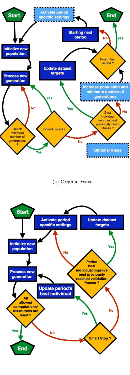
PROPOSED METHOD
Figure 1 depicts the logic of both the original and en-hanced versions of the Wave system. In this section, we de-scribe various components of the enhanced paradigm. Some of these techniques such as smart stopping of periods apply to all Wave configurations, whereas others are used only in specific setups. Table 2 outlines these details.
3.1
Partial Population Renewal
Previously, the entire population was renewed at the be-ginning of a new period. In this study we only renew 80%
of the original population1; the 20% of individuals that are
not replaced are randomly selected. As discussed earlier, the fresh individuals at the start of a new period do not neces-sarily suffer a disadvantage when pitted against the evolved peers from the previous period: this is because the objective
function has changed2. Unless there is a strong correlation
between the new and old objective functions, the old
indi-viduals do not carry an advantage3. Therefore, unlike the
approach taken in [21], we do not require specialised mecha-nisms such as age of the genotype to preserve the disadvan-taged individuals. Of course, pre-existing individuals who may have had good fitness in the previous period, may ini-tially be unable to solve the redrafted problem. However, we believe that maintaining this genetic material into the gene pool offers the possibility of the emergence of phenomena such as exaptation or reuse of existing modules, while at the same time allowing the new genetic material to flourish.
3.2
Smart Stopping of Wave Periods
Previously, in [13], a period was terminated when the Wave system determined that the period was not signifi-cantly improving the fitness any longer. – if the improve-ment, in terms of the best training fitness, over the two most
recent generations was less than 0.5% of the improvement
over the three generations previous to the two most recent generations.
In this work we investigate a new strategy whereby, in every generation, we also compute the fitness of the best trained individual on a validation set. Suppose O(f,d) rep-resents the objective fitness (or fitness value) of an
indi-vidual functionf on a dataset d, then O(fp(g), vp) is the
objective fitness of the individual fp(g) evaluated over the
validation dataset vp; note fp(g) is the best trained
indi-vidual at generation g of the period p. Considering we
are minimizing the fitness, we then terminate a period if
O(fp(g), vp) > O(fp(g−1), vp). In other words, we stop a
period whenever the validation fitness degrades. Granted,
that the validation fitness may oscillate in future, if the pe-riod is allowed to progress; however, our preliminary inves-tigations revealed that waiting for that to happen did not improve scores on the unseen test data sets.
Often, in our experience, especially when linear scaling is enabled, the validation fitness does not change over many
generations, that is,O(fp(g), vp) =O(fp(g−1), vp); this
rep-1First, we explored replacing only 50% of the population;
however, the population converged very quickly without im-proving the results.
2Renewing the target set ast′=t−f akins here a stressful
ecological change.
3A possible extension of this work is to measure this
cor-relation and adjust the relative proportion of new and old population members accordingly.
(a) Original Wave
(b) Enhanced Wave
resents stasis. We decide to halt the current period if stasis continues for more than 5 consecutive generations; however,
if at any time, an individual that iseligibleto be a part of
the joint solution is produced, we allow the current period
to have another 25 generations4 of stasis5. The eligible
in-dividual is the one that produces the best validation fitness thus far, across all the periods. Formally,
O(fp(g), vp)< min
i=0...p−1O(fi, vi) (2)
.
The same criteria is reapplied, as below, at the end of
the period to check whether this period has producedany
solution that is eligible to be a part of the joint solution:
O(fp, vp)< min
i=0...p−1O(fi, vi) (3)
where fp is the best trained individual at any generation
during the current periodpthat also has the best validation
fitness. Due to the stopping conditions described above, this individual is always present in the penultimate generation of the period. Note, the eligibility criteria to get into the joint solution described here is different from that in the previous implementation of Wave described in section 2.1.
3.3
Adaptive Linear Scaling
Previously, the most effective Wave configuration involved alternating between periods with and without linear scaling. However, our exploratory runs indicate that the success rate of periods with and without linear scaling is not uniform. We also noticed that the success rate of linear scaling is pro-portionally much higher in the first period than in the last period. Moreover, all this is highly dependent on the prob-lem under consideration. So, in this work, we have chosen not to alternate between periods with and without linear scaling. Instead, at the beginning of each period, the sys-tem chooses randomly between these two modes based on their success rate in preceding periods. To achieve this the probability of activating linear scaling for a given period is
P = rLS
rLS+r¬LS where rLS =
LSsuc+1
LStot+1 is the approximate
success rate of periods using linear scaling;LStot is the
to-tal number of periods that used linear scalingthus farand
LSsuc is the number of successful periods that used linear
scaling;r¬LS is the approximate success rate of period not
using linear scaling computed the same way. It is important to note that these counts of various kinds of periods stabilise as the number of periods grow thus giving a more reliable measure of the probability of activating linear scaling.
4.
EXPERIMENTS
4.1
Benchmarks
We compare Wave with both EC based and non-EC based machine learning methods. We will use standard GP, both with and without linear scaling to benchmark both the com-putational cost of evolution and accuracy of the resulting models. While we use GSGP [16] and Multiple Linear Re-gression (MLR) solely to benchmark the accuracy of the achieved results. This is because GSGP caches evaluations
4These choices appear adhoc but they are based on some
empirical success; however, they are not necessarily optimal.
5Note, we still stop the period at any time the validation
fitness degrades.
from the first generation and does not evaluate new mate-rial afresh; instead, this work does not cache evaluations yet and therefore can not compare with GSGP. Also, MLR is well known to be far cheaper than GP yet has recently been proposed as a tough benchmark for GP to beat [1].
4.2
Problem Suite
For this study we have used three multi-dimensional datasets from the UCI Machine learning repository [2] together with two mathematical functions. The following datasets from the UCI repository are used:
• Concrete Strength where the objective is to
pre-dict the compressive strength of concrete and data-set includes 1030 instances each having 8 inputs.
• Yachtwhere the objective is to predict the
hydrody-namic performances of a yacht, and data-set includes 308 instances each with 7 inputs.
• Powerplantwhere the task is to predict the net hourly
electrical energy output of a power plant and data-set includes 9568 instances and 4 inputs.
The two mathematical functions chosen are:
• Poly-10 [22]y=x1∗x2 +x3∗x4 +x5∗x6 +x1∗
x7∗x9 +x3∗x6∗x10 and
• Div-5 [23]y= 10 5+P5
i=1(xi−3) 2.
For each of the two mathematical functions, 500 data points in the range [0; 1] are randomly generated. For each run we randomly split the given data-set into three subsets of equal size for training, validation and testing purposes, that is, Ntraining =Nvalidation = Ntesting. For the benchmark
algorithms, because they do not use periods and therefore
can not use a validation set the way we do here6, the
in-stances in the validation set are added to the training set, the numbers of testing instances remains of course the same between the benchmarks and Wave.
Previously, in [14] the Wave system did worse than stan-dard GP on the Yacht problem. As Wave had done bet-ter on all of the other datasets we are inbet-terested in under-standing the cause of the difference in performance. We sus-pect that the relatively small size of the Yacht dataset (308 data points) may have contributed to higher over-fitting. In order to examine this hypotheis we select the Concrete Strength dataset on which Wave performed well and cre-ate a smaller version of this dataset to use as a surrogcre-ate. Thus, we conduct separate runs on smaller training sets from the Concrete Strength problem where the Ntraining =
Nvalidation= 103≈308/3. The remaining points make the
test set such thatNtesting= 824≈1030−206. We will
re-fer to this particular configuration as theSmall Concrete
configuration from now on.
4.3
Common Parameters
The parameters described in Table 1 have been chosen to be the same as in [14] and are consistently applied across all Wave and other GP benchmark experiments. We process 45 runs for each EC configuration for each dataset. Because of
6Exploratory experiments also indicated that standard GP
its low computational cost we performed 100 MLR runs on each dataset.
Table 1: GP Parameters.
Parameter Value
Population 500 individuals
Replacement Strat-egy
Generational
Operator Probabili-ties
Xover: 0.9; Point mutation: 0.1
Tournament Size 10a
Max. depth 17
Max. size 100
Functions set +,−,×,÷(Protected division)
Terminal set Inputs and constants -1.0, -0.5, 0.0, 0.5 & 1.0
Fitness RMSE
Initialisation Ramped half & half Max. initial depth 8
Mutation Step
(GSGP Only)
0.1b
a
A relatively high tournament size but recently successfully used in [6] and [17]; we kept the default tournament size of 3 on GSGP.
b
This is the default mutation step in the implementation proposed in [4].
4.4
Experimental Configurations
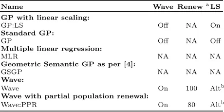
In this paper we study two Wave configurations using both adaptive linear scaling and smart stopping: the first config-uration does not use any optional settings; the second one uses partial population renewal. All of these configurations and benchmarks are described in Table 2.
Table 2: Different Wave and benchmarks configurations.
Name Wave Renewa
LS
GP with linear scaling:
GP:LS Off NA On
Standard GP:
GP Off NA Off
Multiple linear regression:
MLR NA NA NA
Geometric Semantic GP as per [4]:
GSGP NA NA NA
Wave:
Wave On 100 Altb
Wave with partial population renewal:
Wave:PPR On 80 Altb
a
Proportion of population renewed at the beginning of each period. b
Alternation between LS and non-LS periods, based on LS and non LS success rate.
4.5
Performance Metrics
It is not relevant to compare the Wave approach with con-ventional GP simply by measuring the performance of each on the same number of generations. This is because the population is regularly renewed in Wave so that individu-als do not have the same opportunity to bloat as they do in conventional GP. Consequently, each generation is gen-erally less computationally expensive to process with Wave. Therefore, we believe that it would not be equitable to take an approach of terminating runs after the same number of generations for each method, nor to compare statistics mea-sured every generation.
We choose to use the total costC of computed nodes as
a measure of computational cost of a run. Typically, the computational cost of a Wave run will be:
C=
gtot
X
g=1
(
pop
X
i=1
Ntraining×SI
gi) +Nvalidation×SBIg (4)
where pop (population size) is 500 individuals, SIgi is the
size of the ith individual Igiof the generationgand SBIgi
is the size of the best individual at generationginstead, for
classic GP:
C=
gtot
X
g=1
pop
X
i=1
N×SI
gi (5)
where N is the size of the full data set. To ensure equity of resources allocated to different systems, we stop a run when
its computational cost reaches a maximum valueCmax. We
chose7 :
Cmax=k×(Nvalidation+Ntraining) (6)
wherek is a factor chosen so that a run of classic GP with
a population of 500 individuals without linear scaling
con-tinues for approximately 100 generations. Here we used
k= 4000000 forConcreteandSmall Concreteandk=
2000000 forYacht,powerplant,Div-5andPoly-10. Those
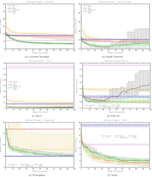
values have been chosen to roughly bring standard GP close to 100 generations, except on Powerplant where we choose a smaller value to cater for its high computational cost due to the size of the dataset (9568 instances). On all datasets and with all parameters we report median testing fitness on a 95% confidence interval in Figure 2.
We observe the statistics at intervals of Cmax/100 and
we call these intevals steps from now on. Nevertheless we
only report a single testing value at every step for MLR and GSGP. Of course MLR is not an EC method, there-fore it was not possible to report gradual progress. Also, because, as stated in [4], GSGP cached node evaluations, we could not come up with an identical budget for GSGP. However, so as not to put it to a disadvantage, we choose a tougher benchmark from GSGP: we benchmark the Wave
results against thebesttest fitnesseverachieved by GSGP
during 2000 generations. Notice, this guards against any over-fitting that GSGP might have experienced and there-fore, avoids the pitfall of choosing an inopportune time to report the testing fitness. In fact, as the results show, GSGP mostly achieved its best test fitness well before reaching the end of run; while there is no guarantee that testing fitness can not improve again, conventional wisdom suggests that overfitting is likelier if we extend the GSGP runs any further.
5.
RESULTS AND DISCUSSION
5.1
Population Renewal
To study the effects of our partial population renewal set-ting, Wave:PPR, we report the earliest period at which the ancestors of the last eligible individual were created. As shown in Table 3, a majority of the last eligible individuals added as part of the joint solution have an ancestor created in the first period. Considering the number of periods re-ported in Table 4 and that we renew 80% of the individuals each period, this result was not obvious. We suspect that this is possibly partly due the relatively large tournaments used, but it also indicates that the genetic material of indi-viduals evolved to address the first objective function still plays a role later on when the objective function has been
7N
validation+Ntrainingis constant on the same dataset for
modified. This may indicates successful events of exapta-tion.
Table 3: Proportion of last eligible individuals included in the joint solution who have an ancestor that was created in the first period.
Concrete Small Yacht Powerplant Div-5 poly-10
Strengh Concrete
73% 76% 62% 73% 77% 58%
5.2
Self-adaptation
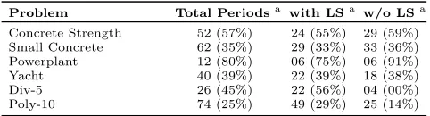
Looking at Table 4, we see that the number of periods executed and the proportion of them which use linear scaling varies greatly depending on the problem. The use of smart stopping of periods and adaptive linear scaling allows Wave to automatically configure itself depending on the problem.
Table 4: Average number and success rate of periods calcu-lated with and without LS for Wave:PPR.
Problem Total Periodsa
with LSa
w/o LSa
Concrete Strength 52 (57%) 24 (55%) 29 (59%)
Small Concrete 62 (35%) 29 (33%) 33 (36%)
Powerplant 12 (80%) 06 (75%) 06 (91%)
Yacht 40 (39%) 22 (39%) 18 (38%)
Div-5 26 (45%) 22 (56%) 04 (00%)
Poly-10 74 (25%) 49 (29%) 25 (14%)
a
Number of periods followed by their success rate in brackets.
5.3
Overfitting
As it can be seen by comparing Figures 2a and 2b, the size of the training dataset influences over-fitting. This assump-tion is reinforced by the absence of over-fitting in Figure 2e where the size of the dataset used is relatively large at 9568 data-points. However, Figures 2c and 2d show that factors other than just the data sizes also affect overfitting; these figures correspond to two datasets, Div-5 and Poly-10, that are identical in size and result from sampling mathematical functions without adding noise and only one them, Poly-10, generate over-fitting.
5.4
Computational Cost
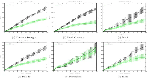
Wave:PPR is the only method tested whose performance either exceeds or equals that of classic GP methods across all datasets at every step. Therefore, Wave:PPR outper-forms standard GP both with and without linear scaling. Wave:PPR also produces the smallest joint solutions among Wave settings as depicted in Figure 3.
5.5
Performances
Because of the nature of GSGP and MLR it was not pos-sible to do a step by step comparison with Wave. From step 40 onwards Wave:PPR performs as well as MLR on the Powerplant problem and outperforms MLR on all the other datasets except Small Concrete. The best median testing fitness of best individuals is reached by GSGP well before the latest generation on 4 out of 6 datasets (Yacht: gen 1; Small Concrete: gen 1112; Div-5: gen 600; Poly-10: gen 472), so it is very unlikely that GSGP could improve its result with more computational resources (higher number of generations) on those datasets. From step 10 onwards Wave:PPR performs as well as or better than GSGP on those four problems. It is hard to conclude on the two remaining
problems because both Wave:PPR and GSGP reached their lowest median testing fitness at the end of the simulation which means both of them could probably improve their re-sults with more computational resources. But we note that Wave:PPR outperforms GSGP from step 10 onwards while on powerplant the final Wave:PPR testing fitness is statisti-cally equivalent to GSGP reported results. It is also worth noting, that the final testing fitness with Wave:PPR is bet-ter than or equal to the best results available (the lowest point of the fitness curve - therefore non-potentially dam-aged by over-fitting) in a previous investigation by Meder-nach et al. [14]; although, the previous study has some ex-perimental differences in terms of computational cost with the work reported here.
6.
CONCLUSIONS
In this paper, we present several improvements to the pre-viously proposed Wave GP method. Based on the results obtained, the proposed changes make Wave more efficient on the given problems and allow it to adapt to their char-acteristics. In particular, Wave successfully demonstrates
exaptationby utilising the older individuals evolved during the previous periods to train against a new objective func-tion; this approach, that we termed as Wave:PPR, seems robust as only multiple linear regression (MLR) performs better than Wave:PPR and that too on one of the problems only. Notice, MLR has been flagged as a tough benchmark for standard GP in recent literature. Additionally, the use of a validation set has improved Wave of ability detect periods of stasis.
7.
REFERENCES
[1] Ignacio Arnaldo, Krzysztof Krawiec, and Una-May O’Reilly. Multiple regression genetic programming. In
Proceedings of the 2014 conference on Genetic and evolutionary computation, pages 879–886. ACM, 2014. [2] Kevin Bache and Moshe Lichman. Uci machine
learning repository, 2013.
[3] Daniel G Blackburn. Saltationist and punctuated equilibrium models for the evolution of viviparity and
placentation.Journal of Theoretical Biology,
174(2):199–216, 1995.
[4] Mauro Castelli, Sara Silva, and Leonardo Vanneschi. A c++ framework for geometric semantic genetic
programming.Genetic Programming and Evolvable
Machines, 16(1):73–81, 2014.
[5] Jeannie Fitzgerald and Conor Ryan. Validation sets for evolutionary curtailment with improved
generalisation. InConvergence and Hybrid Information
Technology, pages 282–289. Springer, 2011.
[6] Ivo Goncalves and Sara Silva. Balancing learning and overfitting in genetic programming with interleaved sampling of training data. In Krzysztof Krawiec, Alberto Moraglio, Ting Hu, A. Sima Uyar, and Bin
Hu, editors,Proceedings of the 16th European
Conference on Genetic Programming, EuroGP 2013,
volume 7831 ofLNCS, pages 73–84, Vienna, Austria,
3-5 April 2013. Springer Verlag.
5 10 15 20 25 30 35
0 10 20 30 40 50 60 70 80 90 100
Median Fitness
Steps Processed Testing Fitness - Concrete
GP:LS GP Wave Wave:PPR GSGP MLR
(a) Concrete Strength
10 15 20 25 30 35
0 10 20 30 40 50 60 70 80 90 100
Median Fitness
Steps Processed Testing Fitness - Small Concrete
GP:LS GP Wave Wave:PPR GSGP MLR
(b) Small Concrete
0 0,1 0,2 0,3 0,4 0,5 0,6 0,7 0,8
0 10 20 30 40 50 60 70 80 90 100
Median Fitness
Steps Processed Testing Fitness - Div-5
GP:LS GP Wave Wave:PPR GSGP MLR
(c) Div-5
0,1 0,2 0,3 0,4 0,5 0,6 0,7 0,8
0 10 20 30 40 50 60 70 80 90 100
Median Fitness
Steps Processed Testing Fitness Poly-10
GP:LS GP
Wave Wave:PPR
GSGP MLR
(d) Poly-10
0 5 10 15 20
0 10 20 30 40 50 60 70 80 90 100
Median Fitness
Steps Processed Testing Fitness - Powerplant
GP:LS GP
Wave Wave:PPR
GSGP MLR
(e) Powerplant
2 4 6 8 10 12 14 16
0 10 20 30 40 50 60 70 80 90 100
Median Fitness
Steps Processed Testing Fitness - Yacht
GP:LS GP
Wave Wave:PPR
GSGP MLR
(f) Yacht
0 500 1000 1500 2000 2500 3000
0 10 20 30 40 50 60 70 80 90 100
Nodes
Steps Processed Global Solution Size
Wave Wave:PPR
(a) Concrete Strength
0 500 1000 1500 2000 2500 3000
0 10 20 30 40 50 60 70 80 90 100
Nodes
Steps Processed Global Solution Size
Wave Wave:PPR
(b) Small Concrete
0 100 200 300 400 500 600 700 800 900
0 10 20 30 40 50 60 70 80 90 100
Nodes
Steps Processed Global Solution Size
Wave Wave:PPR
(c) Div-5
0 200 400 600 800 1000 1200 1400 1600 1800
0 10 20 30 40 50 60 70 80 90 100
Nodes
Steps Processed Global Solution Size
Wave Wave:PPR
(d) Poly-10
0 100 200 300 400 500 600 700
0 10 20 30 40 50 60 70 80 90 100
Nodes
Steps Processed Global Solution Size
Wave Wave:PPR
(e) Powerplant
0 200 400 600 800 1000 1200 1400
0 10 20 30 40 50 60 70 80 90 100
Nodes
Steps Processed Global Solution Size
Wave Wave:PPR
(f) Yacht
Figure 3: Median Size of Overall solution - 95% confidence interval.
[8] Stephen Jay Gould and Elisabeth S Vrba. Exaptation-a missing term in the science of form.
Paleobiology, pages 4–15, 1982.
[9] Eva Jablonka, Marion J Lamb, and Anna Zeligowski.
Evolution in Four Dimensions, revised edition: Genetic, Epigenetic, Behavioral, and Symbolic Variation in the History of Life. MIT press, 2014. [10] Maarten Keijzer. Improving symbolic regression with
interval arithmetic and linear scaling. InGenetic
programming, pages 70–82. Springer, 2003.
[11] John R Koza.Genetic programming: on the
programming of computers by means of natural selection, volume 1. MIT press, 1992.
[12] Barbara McClintock.The significance of responses of
the genome to challenge. Singapore: World Scientific Pub. Co, 1993.
[13] David Medernach, Jeannie Fitzgerald, R. Muhammad Atif Azad, and Conor Ryan. Wave: A genetic programming approach to divide and conquer. In
Proceedings of the Companion Publication of the 2015 Annual Conference on Genetic and Evolutionary Computation, GECCO Companion ’15, pages 1435–1436, New York, NY, USA, 2015. ACM. [14] David Medernach, Jeannie Fitzgerald, R. Muhammad
Atif Azad, and Conor Ryan. Wave: Incremental
erosion of residual error. InProceedings of the
Companion Publication of the 2015 on Genetic and Evolutionary Computation Conference, pages 1285–1292. ACM, 2015.
[15] Brook G Milligan. Punctuated evolution induced by
ecological change.American Naturalist, pages
522–532, 1986.
[16] Alberto Moraglio, Krzysztof Krawiec, and Colin G Johnson. Geometric semantic genetic programming. In
Parallel Problem Solving from Nature-PPSN XII, pages 21–31. Springer, 2012.
[17] R. Muhammad Atif Azad, David Medernach, and Conor Ryan. Efficient approaches to interleaved sampling of training data for symbolic regression. In
Nature and Biologically Inspired Computing (NaBIC), 2014 Sixth World Congress on, pages 176–183. IEEE, 2014.
[18] Thi Hien Nguyen, Xuan Hoai Nguyen, Bob McKay, and Quang Uy Nguyen. Where should we stop? an investigation on early stopping for gp learning. In
Simulated Evolution and Learning, pages 391–399. Springer, 2012.
[19] Luiz OVB Oliveira, Fernando EB Otero, Gisele L Pappa, and Julio Albinati. Sequential symbolic regression with genetic programming. 2014.
[20] Nir Oren.Improving the effectiveness of information
retrieval with genetic programming. PhD thesis, 2002. [21] Ludo Pagie and Paulien Hogeweg. Evolutionary
consequences of coevolving targets.Evolutionary
computation, 5(4):401–418, 1997.
[22] Riccardo Poli. A simple but theoretically-motivated method to control bloat in genetic programming. In
Genetic programming, pages 204–217. Springer, 2003. [23] Ekaterina J Vladislavleva, Guido F Smits, and Dick
Den Hertog. Order of nonlinearity as a complexity measure for models generated by symbolic regression
via pareto genetic programming.Evolutionary
Computation, IEEE Transactions on, 13(2):333–349, 2009.