Type of the Paper (Article)
1
Application of a Hybrid Method for Power System
2
Frequency Estimation with a 0.2-second Sampled Period
3
Chih-Hung Lee 1,* and Men-Shen Tsai 2, 3
4
1 Graduate Institute of Mechanical and Electrical Engineering, National Taipei University of Technology, Taipei,
5
Taiwan; [email protected]
6
2 Graduate Institute of Automation Technology, National Taipei University of Technology, Taipei, Taiwan;
7
8
3 Research Center of Energy Conservation for New Generation of Residential, Commercial, and Industrial Sectors;
9
* Correspondence: [email protected]; Tel.: +886-2-2771-2171(ext. 4374)
10
11
Featured Application: Authors are encouraged to provide a concise description of the specific
12
application or a potential application of the work. This section is not mandatory.
13
Abstract: The signal processing technique is one of the principal tools for diagnosing power quality (PQ)
14
issues in electrical power systems. The Discrete Fourier Transform (DFT) is a frequency analysis technique
15
used to process power system signals and identify PQ problems. However, the DFT algorithm may lead to
16
spectral leakage and picket-fence effect problems for asynchronously sampled signals that contain harmonic,
17
inter-harmonic, and flicker components. To resolve this shortcoming, a hybrid method for frequency
18
estimation based on a second-level DFT approach and a frequency-domain interpolation algorithm to obtain
19
the accurate fundamental frequency of a power system is proposed in this paper. This method uses a
second-20
level DFT to compute the cosine and sine parts for the fundamental frequency components of the acquired
21
signals. Then, a frequency-domain interpolation approach is adopted to determine the amplitude ratio for the
22
cosine and sine parts of the system's fundamental frequency. To demonstrate the performance of the proposed
23
frequency estimation method, the observation window used by this paper to evaluate different estimation
24
algorithms is 200 ms. According to the IEC standards, a 200 ms acquisition window is recommended for
25
power system quality assessment. A set of mixed signals with harmonic, inter-harmonic, and flicker
26
components with the fundamental frequency deviation is used. The evaluation results demonstrate the
27
superiority of the new method over other approaches for assessing asynchronously sampled signals
28
contaminated with noise, harmonic, inter-harmonic, and flicker components.
29
Keywords: frequency estimation, asynchronously sampled, harmonic, flicker.
30
31
1. Introduction
32
Power system signal analysis is a key step in PQ diagnosis. Effective extraction of power system signal
33
features is helpful to understand the underlying physical nature of PQ’s phenomena, and to evaluate its health
34
condition, thereby providing convincing evidences for diagnosis. However, in both academic researches and
35
engineering practices, power system signals are usually highly intricate. The vast increase usage in electronic
36
devices may cause PQ problems such as harmonics, inter-harmonics, and voltage flickers in power systems.
37
Such PQ problems may lead to power system, factory equipment, and public facility deviations or may even
38
result in electrical equipment damage in severe cases.
39
The power system frequency is nonstationary. The degree of frequency change depends on the balance
40
between power generation and load demand. Thus, the frequency is a key indicator for the safety and economy
41
of the power system operation. A frequency below the nominal value represents an overloaded system; while a
42
frequency above the nominal value represents a power oversupply. In general, the power system frequency is a
43
critical indicator for power system monitoring, control, and protection [1-5]. Therefore, power system signal
44
analysis is a key research topic and plays an important role in PQ diagnosis. International standards such as
45
IEC-61000 have described the diagnosis of PQ.
46
In the past, several researches have successfully shown that the frequency assessment technology was able
47
to detect the PQs of defects in power system. These technologies include Zero-crossing Algorithm [5-7],
48
Discrete Fourier Transform (DFT) [8-13], Kalman Filter (KF) [14, 15], Phase-Locked Loops (PLL) [16, 17],
49
Newton Algorithm [18, 19], Least squares Algorithm (LMS) [20, 21], Prony Algorithm [4, 22], Taylor
50
Algorithm [23, 24], and Artificial-intelligence Algorithm [25, 26].
51
Among them, one of the two most popular techniques adopted is the Zero-crossing Algorithm, which has
52
the least computational complexity and the fastest execution speed. However, this method is susceptible to noise
53
and spikes, and can only provide an accurate frequency evaluation in noise-free and disturbance-free
54
environments [5-7].
55
In [5], using the waveform construction method to combine the Time Domain Frequency Estimation
56
Algorithm with the Newton Interpolation method was proposed. This approach can eliminate the leakage effect
57
caused by the FFT (Fast Fourier Transform) calculation under asynchronous sampling conditions. In this paper,
58
a Time Domain Zero-crossing Algorithm to evaluate the basic frequency is proposed. This algorithm uses the
59
zero-crossing frequency detection method to calculate the basic frequency. Because this algorithm can be
60
affected by non-basic frequency signals, a pre-filter must be used to eliminate the non-basic frequency signals.
61
After the basic frequency has been obtained, Newton Interpolation method is applied to generate a new sample
62
waveform that conforms to the FFT application conditions. As a result, the accurate basic frequency under
63
asynchronous sampling conditions can be obtained.
64
In [6, 7], the authors proposed the digital filter and zero-crossing technique combination frequency
65
evaluation method. They broke down the original sample signals into two orthogonal component waveforms
66
using cosine and sine filters. These two waveforms and the zero-crossing technique are used to assess the basic
67
frequency of the power system. The results indicated that the orthogonal filter and the zero-crossing technique
68
can effectively reduce the noise and disturbance interferences.
69
The other technique that is popular used in calculating the fundamental frequency of a power system is
70
DFT/FFT. In the IEC61000-4-30 standard, PQ measurement analysis is mostly based on DFT/FFT techniques.
71
DFT/FFT can convert the periodic signals obtained via synchronous sampling into frequency domain data to
72
help us learn more about the spectrum composition. However, the basic frequency of an actual power system
73
will vary from time to time and become affected by noise, flickers, harmonic waves, inter-harmonic waves, and
74
other disturbances. Therefore, it is unrealistic and impossible to achieve strict synchronous sampling without a
75
special technique such as PLL (Phase Lock Loop). Asynchronous sampling would cause the DFT/FFT
76
algorithm to create the spectral leakage and picket-fence effect problems and directly cause the FFT algorithm
77
spectrum calculation accuracy to drop dramatically [8–13].
78
In [8], it was proposed to use the window method with DFT for frequency calculation, and to obtain the
79
basic frequency parameter values according to the multi-point spectrum near the base frequency peak point as
80
well as the Hanning window interpolation expressed as a function of the frequency domain itself. The results
81
indicated that this multi-point frequency domain interpolation algorithm can effectively reduce the noise and
82
disturbances.
83
Reference [9] adopted the pseudo-synchronization technique, Hanning window, and FFT combination for
84
frequency calculation in order to improve the frequency estimation accuracy under the noise and disturbance
85
effects. The author combined the original sample signals with the Hanning window function, performed FFT
86
conversion for the new wave signals, and then assessed the basic frequency of the power system. The results
87
indicated that the pseudo-synchronization technique combined with FFT can effectively reduce the noise and
88
disturbances.
89
The PQ event detection algorithms require precise power system frequency which can be obtain using
90
DFT-based frequency estimation algorithms under asynchronously-sampled signals that are contaminated with
91
noise, flicker, and harmonic and inter-harmonic components. In this paper, we proposed a two-level DFT and
92
frequency domain interpolation hybrid method to accurately calculate the basic frequency of a power system.
93
This paper is divided into four chapters. Chapter 1 is the preface. Chapter 2 explores the two-level DFT and
94
frequency domain interpolation hybrid method. Chapter 3 provides validation for the method. Chapter 4
95
concludes this paper.
96
2. Two-Level DFT and Frequency Domain Interpolation Hybrid Method
97
Frequency evaluation technology is the foundation of PQ analysis and monitoring. Therefore, excellent
98
frequency assessment techniques can improve power system protection and monitoring. At present, the
99
IEC61000-4-30 standard established by the International Electrotechnical Commission (IEC) for power
quality-100
the standard and facilitate development, numerous monitoring devices have adopted the fixed sampling
102
frequency-based DFT technique in order to simplify device design. However, the basic electricity frequency
103
changes may lead to asynchronous sampling problems for fixed sampling frequency devices, which may cause
104
leakage effects during the DFT calculations. In addition, if the sampling frequency and calculation method
105
window are not divisible, it would also cause the DFT method to obtain inaccurate basic frequencies.
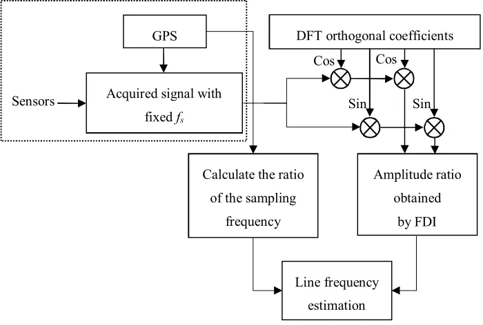
106
The primary implementation steps of this paper are shown in Figure 1. First, we calculated the DFT
107
orthogonal coefficient and amplitude ratio deviation coefficient based on the power signals captured. Next, we
108
created two levels of orthogonal filtering based on the DFT orthogonal coefficients and power signals
109
calculated. We then used the two orthogonal filtering signals and frequency domain interpolation to determine
110
the amplitude ratio needed for the frequency calculation. Finally, we used the amplitude ratio and the amplitude
111
ratio deviation coefficient to calculate the frequency more precisely.
112
113
Figure 1. Proposed frequency assessment process.
114
115
2.1. DFT Orthogonal Filter Coefficients
116
The actual power system signals (such as voltage and current) can be expressed in discrete time with three
117
parameters: amplitude (A), frequency (f), and phase (θ), as shown in Equation (1).
118
119
0 0
1 ,... 1 , 0 , 2
cos
N f f
N n
f n f A
n x
s
s a
(1)
In (1), fs is the sampling frequency, f0 is the nominal frequency, fa is the actual frequency, N0 is the number
120
of samples per cycle, and N is the total number of samples.
121
We used the DFT to convert the sample's N-point discrete signals into the N-point spectrum energy. The
122
DFT formula is shown in Equation (2).
123
)]
sin(2
)
(
)
2
cos(
)
(
[
2
)
(
0 0 1
0 n 0
0 1
0 n
n
N
f
f
n
x
j
n
N
f
f
n
x
N
i
X
aN a
N
(2)Assuming there is a single window with M-point samples,
Equation
(2) can be expanded as follows:124
Calculate the ratio
of the sampling
frequency Acquired signal with
fixed fs
Amplitude ratio
obtained
by FDI
GPS DFT orthogonal coefficients
Sensors
Line frequency
estimation
Cos Cos
)
2
sin(
)
(
...
)
4
sin(
)
2
(
)
2
sin(
)
1
(
2
)
2
cos(
)
(
...
)
4
cos(
)
2
(
)
2
cos(
)
1
(
2
)
X(
0 0 0 0 0 0 0 0 0 0f
f
M
x
N
f
f
x
N
f
f
x
M
j
f
f
M
x
N
f
f
x
N
f
f
x
M
i
a a a a a a
(3)Therefore, for the
i-
th data window, the sine and cosine components can be expressed as
125
Equations (4) and (5).
126
1n 0 0
) 2 cos( ) ( 2 ) ( i M i a n N f f i x M i
A (4)
1n 0 0
) 2 sin( ) ( 2 ) ( i M i a n N f f i x M i
B (5)
If the fundamental signal frequency is equal to the assumed basic frequency (fa=f0), then Equations (4)
127
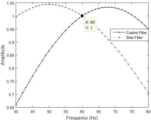
and (5) are orthogonal to each other. At this point, A(t) and B(t) represent pure cosine and pure sine wave forms,
128
respectively. In Figure 2, the orthogonal filter has different amplitude responses for all frequencies other than
129
the nominal frequency. Its different amplitude response results clearly indicated that, when the orthogonal filter
130
conforms to fa=f0 (60 Hz), the amplitude response value is 1.
131
132
Figure 2. Frequency impact of the orthogonal filter.
133
2.2. Frequency Estimation Algorithm
134
In summary, we can derive the frequency change rules based on the amplitude response characteristics
135
described above, and thus calculate the exact frequency. In practical applications, the usable vector lengths for
136
the cosine and sine coefficients of the two orthogonal filters have the vector matrix of N0 as expressed by
137
Equations (6) and (7).
138
2 os(2 ), os(4 ), os(2 1 ) os(2 ) 0 0 0 0 0 0 0 0 0 N c N N N c N N c N N c N
CosWindow (6)
2 sin(2 ),sin(4 ), sin(2 1 ) sin(2 ) 0 0 0 0 0 0 0 0
0 N N N
N N N N N N
SinWindow (7)
Performing unilateral Z conversion for Equations (6) and (7), their amplitude response functions can be
139
0 0 0 0 0 0 0 0 2 cos 2 cos sin sin cos 4 N f f N f f f f N N N f HCosWindow (8)
0 0 0 0 0 0 00 cos 2 cos 2
sin cos sin 4 N f f N f f f f N N N f HSinWindow (9)
Equations (8) and (9) can be used to derive the amplitude ratio of the two filters, and this ratio can be
141
expressed as Equation (10).
142
0 0 0 tan tan N f f N f H f H B A R SinWindow CosWindow atio (10)Finally, the basic power signal frequency can be deduced using the amplitude value obtained using
143
Equation (10), and the basic power signal frequency is shown as Equation (11).
144
atio a R N N f f 0 1 00 tan tan
(11)
However, the filtered signals can be affected by the amplitude responses and the frequency response
145
effects. Therefore, the frequency evaluation using Equations (10) and (11) will be subject to these factors.
146
Equations (12) and (13) are phase response equations that can be used to deduce the 90˚ angle differences. Thus,
147
we can resolve the phase angle differences and find the ideal amplitude ratios.
148
0 0 0 1 f N f N f HCosWindow (12)
0 0 0 1 2 1 f N f N f HSinWindow (13)
To resolve the phase response effects, a DFT filter is used to determine the amplitude ratio of the filtered
149
sine and cosine signals outputted during the first level. This method uses the phase response characters to offset
150
the filtered signal by 90˚ to turn the signal phase difference into 180˚. Thus, the two orthogonal signals will
151
become symmetrical signals with only the positive and negative sign differences. The vectors of the second
152
level DFT-filtered discrete signals are represented as Equations (14) and (15).
153
T n A A A AA[ 1 2 3 ... ] (14)
T n B B B B
B [ 1 2 3 ... ] (15)
When Equation (10) uses Equations (14) and (15) to calculate the amplitude ratio, the amplitude ratio
154
would have a significant deviation in the vicinity of the zero-crossover for the filtered values A and B, and the
155
frequency calculation would produce an erroneous value. To resolve the zero-crossover problem, the frequency
156
domain difference technique is adapted to verify the amplitude ratio because, in addition to the harmonic or
157
inter-harmonic waves, real signals also contain voltage flickers and other noises. Although this frequency
158
assessment method is based on the DFT filtering technique and can prevent harmonic and inter-harmonic wave
159
interferences, the method still cannot prevent voltage flickers and other signal noise interferences. Thus, the
160
interpolation technique is applied to further suppress the interferences and calculate the precise amplitude value.
161
2.3. Amplitude Interpolation Method
164
The discrete time sequence representation of a Hanning window is expressed as [8, 9]:
165
0.5 0.5cos 2 , 0,1,... 1
n N
N n n
W (16)
166
The spectrum of the dot product of x(.) from Equation (1) and the W(.) from Equation (16) yields Equation
167
(17):
168
1 ( )
2
, 0,1,... 1
j j
X k Ae W k Ae W k
j
k N
(17)
169
where k is the frequency index of the DFT at the k-th spectral line; λ is the normalized frequency and can
170
be written in two parts, as indicated in Equation (18) where l is the integer part of the frequency and δ is the
171
fraction part of the frequency.
172
0 0
, 0.5 0.5
f N l
f N
(18)
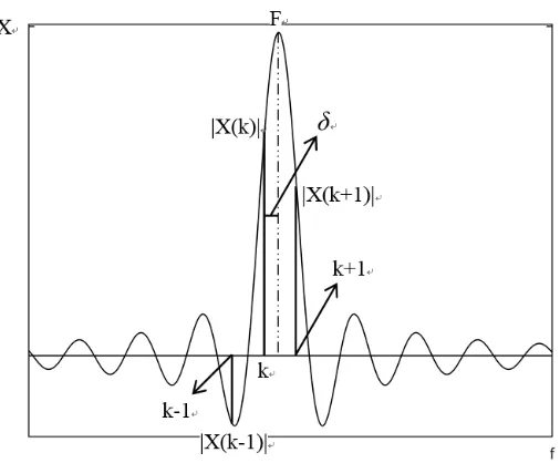
173
Figure 3 shows the interpolation method of the Fourier transform spectrum where k is the largest index
174
value in the Xk amplitude. When N is large enough, the amplitude can be expressed as:
175
2 sin
X N A
Vk k (19)
176
δ is the largest frequency deviation for the true amplitude and the transformed amplitude in the spectrum,
177
the value range of δ is between -0.5–0.5, the left and the right maximum amplitudes have the index values of
k-178
1 and k+1, and its amplitude is expressed as:
179
1 2
sin 1
1
A N X
Vk k (20)
180
After the sampling signal is multiplied by the Hanning Window, the relationship between the largest
181
amplitude frequency and the second largest amplitude frequency after the transformation—Vk and Vk±1—has
182
the ratio of α which is expressed as:
183
2 1 1
k k
V
V (21)
184
Through the Hanning Window relationship, the deviation ratio δ is expressed as:
185
1 1
2 (22)
186
The amplitude correction value is thus expressed as:
187
VkN V
sin 1
2 2
(23)
Figure 3. Interpolation algorithm diagram.
189
Finally, after the amplitude ratio has been incorporated into the frequency domain interpolation using
190
Equations (14) and (15), Equation (23) is used to calculate the corrected orthogonal filter amplitude, and then
191
incorporate the amplitude value into Equation (11) to accurately evaluate the power system frequency.
192
3. Results
193
To verify the performance of the two-level DFT and frequency domain interpolation hybrid method
194
proposed in this paper, we performed numerical simulations based on the various voltage signals encountered
195
by the actual power system in a MATLAB simulation environment. They include harmonics, inter-harmonics,
196
flickers, noises, and frequency offsets.
197
We used four frequency evaluation methods to compare all of the test results: the zero-crossing
198
interpolation waveform reconstruction method (ZCIWR) [5], the frequency-domain interpolated (FDI) [8], the
199
frequency-domain interpolated waveform reconstruction method (FDIWR) [9], and the method proposed in this
200
paper. The objective of the comparisons is to understand the frequency deviations of the frequency estimation
201
methods. The frequency absolute value proposed in [4, 26] is used to calculate the relative error as described in
202
Equation (24).
203
% 100 Value
Actual
Value Estimated
-Value Actual Error(%)
Relative (24)
204
The IEC 61000-4-7 standard has proposed the 5 Hz frequency resolution recommended value based on
205
the DFT technique. That is, the analysis information with the time length of 0.2 s is applied for harmonic and
206
inter-harmonic analyses. The sampling frequency is 3000 Hz, and the experimental data window length of N is
207
set to 0.2 s. For the ZCIWR method, the frequency can only be calculated near the vicinity of the zero-crossover.
208
To verify the performance frequency evaluation performance, the steady-state data window sliding coefficient
209
was obtained as one cycle, and one frequency calculation was conducted for each cycle. To obtain an accurate
210
and precise conclusion, each simulated measurement was performed 500 times and the average value is used.
211
3.1. Asynchronous Sampling Basic Frequency Evaluation
212
The IEC 61000-4-30 standard specifies the accuracy tolerance for measurements made by PQ analysis
213
instruments. The basic frequency offset tolerance range for a power system with a rated frequency of 60 Hz is
214
between 51 Hz and 69 Hz. To test whether the frequency evaluation method can effectively calculate the basic
215
frequency, the simulated wave is represented using Equation (25), where fa varies between 51 Hz and 69 Hz,
216
and the with 1 Hz offset.
217
t
f t
x cos 2 a (25)
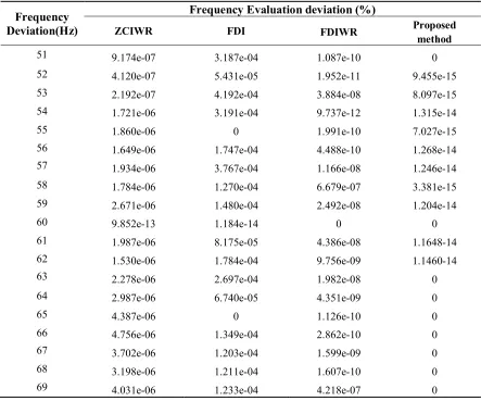
Table 1 shows the results according to different frequencies under the various frequency evaluation
219
methods. As anticipated, the proposed method is not affected by the a-th frequency offsets. Table 1 indicated
220
that the deviations derived from the calculation method proposed by this paper are lower than 1e-14.
221
Table 1. Average relative frequency deviations for different basic frequency offsets.
222
Frequency Deviation(Hz)
Frequency Evaluation deviation (%)
ZCIWR FDI FDIWR Proposed
method
51 9.174e-07 3.187e-04 1.087e-10 0
52 4.120e-07 5.431e-05 1.952e-11 9.455e-15
53 2.192e-07 4.192e-04 3.884e-08 8.097e-15
54 1.721e-06 3.191e-04 9.737e-12 1.315e-14
55 1.860e-06 0 1.991e-10 7.027e-15
56 1.649e-06 1.747e-04 4.488e-10 1.268e-14
57 1.934e-06 3.767e-04 1.166e-08 1.246e-14
58 1.784e-06 1.270e-04 6.679e-07 3.381e-15
59 2.671e-06 1.480e-04 2.492e-08 1.204e-14
60 9.852e-13 1.184e-14 0 0
61 1.987e-06 8.175e-05 4.386e-08 1.1648-14
62 1.530e-06 1.784e-04 9.756e-09 1.1460-14
63 2.278e-06 2.697e-04 1.982e-08 0
64 2.987e-06 6.740e-05 4.351e-09 0
65 4.387e-06 0 1.126e-10 0
66 4.756e-06 1.349e-04 2.862e-10 0
67 3.702e-06 1.203e-04 1.599e-09 0
68 3.198e-06 1.211e-04 1.607e-10 0
69 4.031e-06 1.233e-04 4.218e-07 0
3.2. Basic Frequency Evaluation Under Harmonic and Inter-harmonic Environments
223
In this paper, we referenced the IEC 61000-4-30 standard to propose the harmonic and inter-harmonic
224
verification perimeters. The simulated waveform is represented using Equation (26) where fa ranged from 51
225
Hz to 69 Hz and the offsets were made in 1 Hz increments.
226
25 2
0.05cos
29 2
0.01cos
3.5 2
0.01cos
7.5 2
; cos05 . 0
2 13 cos 05 . 0 2
7 cos 1 . 0 5
cos 05 . 0 2 3 cos 1 . 0 2 cos
t f t
f t
f t
f
t f pi
t f t
f t
f t
f t
x
a a
a a
a a
a a
a
227
(26)
228
Table 2 indicates that all four techniques are affected by the harmonics and inter-harmonics in the
229
harmonic and inter-harmonic environments. However, the average deviations derived from the frequency
230
evaluation algorithm adopted by this paper under a variety of frequency offsets were all better than those of
231
other methods.
232
Table 2. Average relative frequency deviation under harmonic and inter-harmonic environment.
233
Frequency Deviation(Hz)
Frequency Evaluation deviation (%)
ZCIWR FDI FDIWR Proposed
method
52 3.745e-07 4.233e-05 1.361e-05 4.119e-07
53 2.299e-07 4.126e-04 0.002 6.459e-07
54 1.601e-06 3.411e-04 4.764e-05 3.482e-07
55 1.513e-06 2.122e-06 1.565e-05 1.268e-08
56 1.414e-06 2.246e-04 2.939e-05 1.731e-07
57 1.964e-06 3.731e-04 3.879e-05 3.518e-07
58 1.894e-06 8.510e-05 4.630e-05 5.698e-08
59 2.760e-06 1.372e-04 4.218e-05 3.070e-08
60 9.971e-13 1.184e-14 0 0
61 2.025e-06 8.500e-05 4.233-05 4.798-09
62 1.504e-06 1.762e-04 3.616e-04 8.195e-08
63 2.169e-06 2.601e-04 7.604e-04 8.980e-08
64 2.906e-06 7.771e-05 3.063e-04 1.6156e-08
65 4.542e-06 5.025e-07 7.562e-07 1.372e-09
66 5.133e-06 1.456e-04 7.672e-06 1.004e-08
67 3.765e-06 8.755e-05 0.001 8.496e-08
68 3.364e-06 9.517e-05 0.004 3.193e-08
69 3.843e-06 1.318e-04 0.005 7.024e-08
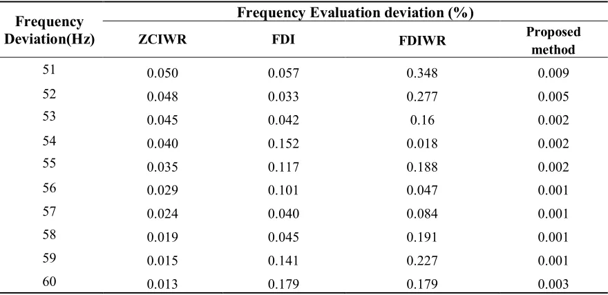
3.3. Basic Frequency Evaluation Under Flickering Environments
234
In addition to the harmonic and inter-harmonic frequencies, power system voltages usually also contain
235
flicker frequencies. According to [27], human eyes are most sensitive to a flicker frequency of approximately
236
8.8 Hz. Thus, we added two flicker components of 5 Hz and 8.8 Hz to Equation (26), with amplitudes of 0.05%
237
and 0.1%, respectively.
238
Table 3 shows the frequency evaluation deviations of the four methods under the harmonic,
inter-239
harmonic, and flicker interference environments. The relative deviation obtained using the method proposed by
240
this paper was approximately 1e-4%, and was approximately 1e-1% using other methods. Thus, the method
241
proposed by this paper has better performance under the harmonic, inter-harmonic, and flicker interference
242
environments.
243
Table 3. Average relative frequency deviation under flicker environments.
244
Frequency Deviation(Hz)
Frequency Evaluation deviation (%)
ZCIWR FDI FDIWR Proposed
method
51 0.050 0.057 0.348 0.009
52 0.048 0.033 0.277 0.005
53 0.045 0.042 0.16 0.002
54 0.040 0.152 0.018 0.002
55 0.035 0.117 0.188 0.002
56 0.029 0.101 0.047 0.001
57 0.024 0.040 0.084 0.001
58 0.019 0.045 0.191 0.001
59 0.015 0.141 0.227 0.001
61 0.014 0.121 0.251 0.009
62 0.017 0.042 0.272 0.010
63 0.020 0.044 0.246 0.011
64 0.024 0.097 0.283 0.006
65 0.028 0.209 0.270 0.008
66 0.031 0.125 0.219 0.010
67 0.034 0.041 0.140 0.011
68 0.036 0.030 0.238 0.005
69 0.050 0.057 0.348 0.009
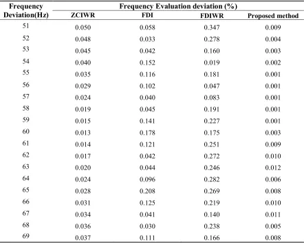
3.4. Basic Frequency Evaluation Under Noise Environments
245
To test whether the frequency estimation algorithm can effectively calculate the basic frequency under a
246
noise interference environment, a 60 dB of noise is added to the simulated waveform discussed in 3.3.
247
Table 4 shows the maximum relevant deviation from simulating all of the frequency estimation methods
248
500 times in mixed environments. The table indicates that when using the ZCIWR, FDI, FDIWR, and the
249
method proposed by this paper in mixed interference environments with a steady-state evaluation frequency of
250
between 51–69 Hz; the maximum average relative deviations were 5e-02%, 2e-01%, 3e-01%, and 1e-02%,
251
respectively. The results indicate that all four algorithms had good responses in the 60 dB environment.
252
Table 4. Maximum relative frequency deviation in a mixed environment.
253
Frequency Deviation(Hz)
Frequency Evaluation deviation (%)
ZCIWR FDI FDIWR Proposed method
51 0.050 0.058 0.347 0.009
52 0.048 0.033 0.278 0.004
53 0.045 0.042 0.160 0.003
54 0.040 0.152 0.019 0.002
55 0.035 0.116 0.181 0.001
56 0.029 0.102 0.047 0.001
57 0.024 0.040 0.083 0.001
58 0.019 0.045 0.191 0.001
59 0.015 0.141 0.227 0.001
60 0.013 0.178 0.175 0.003
61 0.014 0.121 0.251 0.009
62 0.017 0.042 0.272 0.010
63 0.020 0.044 0.246 0.012
64 0.024 0.096 0.282 0.006
65 0.028 0.208 0.269 0.008
66 0.031 0.125 0.219 0.010
67 0.034 0.041 0.140 0.011
68 0.036 0.030 0.238 0.005
69 0.037 0.111 0.166 0.008
254
4. Conclusion
256
In this paper, we adopted the classic spectrum analysis algorithm used by the majority of scholars—DFT—
257
as the basis for frequency evaluation for the PQ analysis. A two-level DFT and frequency domain interpolation
258
hybrid technique is used for basic frequency evaluation. This method used the DFT filter as the basis for the
259
frequency calculation. This approach can reduce the harmonic and inter-harmonic interferences. The orthogonal
260
characteristics and the frequency domain interpolation method were then used to further suppress the flicker
261
components. The experimental results indicated that when the signals sampled using the method proposed by
262
this paper contained harmonic, inter-harmonic, and flicker components, the method can obtain high-precision
263
basic frequency that can be used to facilitate subsequent PQ spectrum analyses.
264
Acknowledgments: This research is supported by the Project of the Ministry of Science and Technology,
265
Taiwan, under grant numbers MOST 104-2221-E-027-060-MY2 and MOST 106-3113-E-006-010.
266
References
267
1. Luo, Y.; Kaicheng, L.; Li, Y.; Cai, D.; Zhao, C.; Meng, Q. Three layer bayesian network for classification of complex
268
power quality disturbances. IEEE Transactions on Industrial Informatics 2017, 1-1
269
2. Camarena-Martinez, D.; Valtierra-Rodriguez, M.; Perez-Ramirez, C.A.; Amezquita-Sanchez, J.P.; Romero-Troncoso,
270
R.d.J.; Garcia-Perez, A. Novel downsampling empirical mode decomposition approach for power quality analysis.
271
IEEE Transactions on Industrial Electronics 2016, 63, 2369-2378.
272
3. Singh, U.; Singh, S.N. Optimal feature selection via nsga-ii for power quality disturbances classification. IEEE
273
Transactions on Industrial Informatics 2017, 1-1.
274
4. Cheng, I.C. Design of measurement system based on signal reconstruction for analysis and protection of distributed
275
generations. IEEE Transactions on Industrial Electronics 2013, 60, 1652-1658.
276
5. Zhou, F.; Huang, Z.; Zhao, C.; Wei, X.; Chen, D. Time-domain quasi-synchronous sampling algorithm for harmonic
277
analysis based on newton's interpolation. IEEE Transactions on Instrumentation and Measurement 2011, 60,
2804-278
2812.
279
6. Djurić, M.B.; Djurišić, Ž.R. Frequency measurement of distorted signals using fourier and zero crossing techniques.
280
Electric Power Systems Research 2008, 78, 1407-1415.
281
7. Chen, Y.-C.; Chien, T.-H. A simple approach for power signal frequency determination on virtual instrument
282
platform. 2015; Vol. 9, p 65-71.
283
8. Agrez, D. Weighted multipoint interpolated dft to improve amplitude estimation of multifrequency signal. IEEE
284
Transactions on Instrumentation and Measurement 2002, 51, 287-292.
285
9. Chang, G.; Chen, C.I.; Liu, Y.J.; Wu, M.C. Measuring power system harmonics and interharmonics by an improved
286
fast fourier transform-based algorithm. 2008; Vol. 2, p 193-201.
287
10. Nam, S.-R.; Kang, S.-H.; Kang, S.-H. Real-time estimation of power system frequency using a three-level discrete
288
fourier transform method. Energies 2015, 8, 79.
289
11. Jun-Zhe, Y.; Chih-Wen, L. A precise calculation of power system frequency and phasor. IEEE Transactions on Power
290
Delivery 2000, 15, 494-499.
291
12. Belega, D.; Petri, D. Accuracy analysis of the multicycle synchrophasor estimator provided by the interpolated dft
292
algorithm. IEEE Transactions on Instrumentation and Measurement 2013, 62, 942-953.
293
13. Macii, D.; Petri, D.; Zorat, A. Accuracy analysis and enhancement of dft-based synchrophasor estimators in
off-294
nominal conditions. IEEE Transactions on Instrumentation and Measurement 2012, 61, 2653-2664.
295
14. Reza, S.; Ciobotaru, M.; Agelidis, V.G. Accurate estimation of single-phase grid voltage fundamental amplitude and
296
frequency by using a frequency adaptive linear kalman filter. IEEE Journal of Emerging and Selected Topics in Power
297
Electronics 2016, 4, 1226-1235.
298
15. Talebi, S.P.; Kanna, S.; Mandic, D.P. A distributed quaternion kalman filter with applications to smart grid and target
299
tracking. IEEE Transactions on Signal and Information Processing over Networks 2016, 2, 477-488.
300
16. Golestan, S.; Guerrero, J.M.; Vasquez, J.C. A pll-based controller for three-phase grid-connected power converters.
301
IEEE Transactions on Power Electronics 2018, 33, 911-916.
302
17. Golestan, S.; Guerrero, J.M.; Vasquez, J.C. A nonadaptive window-based pll for single-phase applications. IEEE
303
Transactions on Power Electronics 2018, 33, 24-31.
304
18. Reza, M.S.; Ciobotaru, M.; Agelidis, V.G. Power system frequency estimation by using a newton-type technique for
305
19. Nanda, S.; Dash, P.K. A gauss–newton adaline for dynamic phasor estimation of power signals and its fpga
307
implementation. IEEE Transactions on Instrumentation and Measurement 2018, 67, 45-56.
308
20. Xia, Y.; Blazic, Z.; Mandic, D.P. Complex-valued least squares frequency estimation for unbalanced power systems.
309
IEEE Transactions on Instrumentation and Measurement 2015, 64, 638-648.
310
21. Ž, Z.; Krstajić, B.; Popović, T. Improved frequency estimation in unbalanced three-phase power system using coupled
311
orthogonal constant modulus algorithm. IEEE Transactions on Power Delivery 2017, 32, 1809-1816.
312
22. Lobos, T.; Rezmer, J. Real-time determination of power system frequency. IEEE Trans. Instrum. Meas.1997, 46,
313
877–881.
314
23. Khodaparast, J.; Khederzadeh, M. Dynamic synchrophasor estimation by taylor–prony method in harmonic
315
and non-harmonic conditions. IET Generation, Transmission & Distribution 2017, 11, 4406-4413.
316
24. Fu, L.; Zhang, J.; Xiong, S.; He, Z.; Mai, R. A modified dynamic synchrophasor estimation algorithm considering
317
frequency deviation. IEEE Transactions on Smart Grid 2017, 8, 640-650.
318
25. Coury, D.V.; Delbem, A.C.B.; Carvalho, J.R.d.; Oleskovicz, M.; Simoes, E.V.; Barbosa, D.; Silva, T.V.d. Frequency
319
estimation using a genetic algorithm with regularization implemented in fpgas. IEEE Transactions on Smart Grid
320
2012, 3, 1353-1361.
321
26. Gupta, P.; Bhatia, R.S.; Jain, D.K. Average absolute frequency deviation value based active islanding detection
322
technique. IEEE Transactions on Smart Grid 2015, 6, 26-35.
323
27. Bai, F.; Wang, X.; Liu, Y.; Liu, X.; Xiang, Y.; Liu, Y. Measurement-based frequency dynamic response estimation
324
using geometric template matching and recurrent artificial neural network. CSEE Journal of Power and Energy
325