Visual Monocular 3D Reconstruction and Component
Identification for Small Spacecraft
Mark Post1,†,‡ ID, Junquan Li2,‡
1 University of Strathclyde, Glasgow, United Kingdom; [email protected] 2 Space Innovation Robotics Ltd, Glasgow, United Kingdom; [email protected] * Correspondence: [email protected]; Tel.: +44-0141-574-5274
† Current address: Department of Design, Manufacture and Engineering Management, University of Strathclyde, 75 Montrose St. Glasgow, United Kingdom, G1 1XJ
‡ These authors contributed equally to this work.
Abstract: A monocular vision pose estimation and identification algorithm used on a small
1
spacecraft for future orbital servicing is studied in this paper. A tracker spacecraft equipped with
2
a short-range vision system is proposed to recover the 3D structural model of a space target in
3
orbit and automatically identify its solar panels and main body using only visual information from
4
an onboard camera. The proposed reconstruction and identification framework is tested using
5
structure-from-motion and point cloud identification methods. The Efficient Perspective-n-Points
6
(EPnP) descriptor is used for pose estimation. Triangulated points are used for component
7
segmentation by means of orientation histogram descriptors. Experimental results based on
8
laboratory images of a spacecraft model show the effectiveness and robustness of our approach.
9
Keywords: spacecraft; structure from motion; monocular vision; component detection; structure
10
analysis
11
1. Introduction 12
Space object 3D reconstruction, pose estimation and identification is very important for spacecraft
13
orbital servicing and space situational awareness based on satellite imaging. Structure from Motion
14
technology and pose estimation has attracted a lot of interest as an enabling technology for detecting,
15
tracking, cataloguing and identifying satellites and spacecraft in recent years. Structure from Motion
16
(SfM) is a method for obtaining 3-D structures using only monocular feature matches between multiple
17
images at multiple angles, which can include lines (e.g. Canny edge detection), corners (e.g. Harris
18
corner detection, and other types of features. It also represents a natural progression into point cloud
19
techniques from feature-based ego-motion estimation between pairs of images. 3D reconstruction and
20
identification has been studied extensively, but in order for such systems to work effectively on small
21
spacecraft with only single visual sensors, the implementation of point cloud building, image feature
22
point matching, sparse reconstruction, identification strategy and dimensional analysis information
23
must be considered.
24
High performance optical imaging sensors-such as radar, lidar, visible and infrared are used for
25
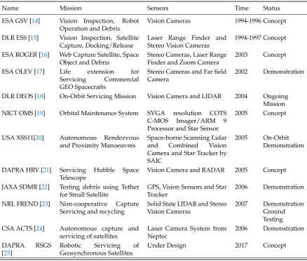
detecting, tracking and identifying objects in orbit. Table1shows a list of existing on-orbit servicing
26
missions and demonstrations. RF radar trades off precision for wide range of operation, and is not as
27
suitable for uncooperative or small targets. The TriDAR system used a LIDAR and Iterative Closest
28
Point system outside the ISS without approach or autonomy [1]. Recent automated rendezvous and
29
docking systems make use of optical, laser ranging, and LIDAR systems [2] [3] and visually-aided
30
systems have been tested in proximity operations with NASA’s Space Shuttle, JAXA’s ETS-VII satellite
31
[4] as well as other satellites such as the DART mission [5]. The Rendezvous Lidar System (RLS) has
32
also been tested on the XSS-11 spacecraft for rendezvous operations. However, the complexity, size,
33
Table 1.Summary of On-Orbit Servicing Missions
Name Mission Sensors Time Status
ESA GSV [14] Vision Inspection, Robot Operation and Debris
Vision Cameras 1994-1996 Concept
DLR ESS [15] Vision Inspection, Satellite Capture, Docking/Release
Laser Range Finder and Stereo Vision Cameras
1994-1997 Concept
ESA ROGER [16] Web Capture Satellite, Space Object and Debris
Stereo Cameras, Laser Range Finder and Zoom Camera
2003 Concept
ESA OLEV [17] Life extension for Servicing Commercial GEO Spacecrafts
Stereo Cameras and Far field Camera
2002 Demonstration
DLR DEOS [18] On-Orbit Servicing Mission Vision Camera and LIDAR 2004 Ongoing Mission NICT OMS [19] Orbital Maintenance System SVGA resolution COTS
C-MOS Imager/ARM 9 Processor and Star Sensor
2005 Concept
USA XSS11[20] Autonomous Rendezvous and Proximity Manoeuvres
Space-borne Scanning Lidar and Combined Vision Camera and Star Tracker by SAIC
2005 On-Orbit Demonstration
DAPRA HRV [21] Servicing Hubble Space Telescope
Vision Camera and RADAR 2005 Concept
JAXA SDMR [22] Testing debris using Tether for Small Satellite
GPS, Vision Sensors and Star Tracker
2006 Demonstration
NRL FREND [23] Non-cooperative Capture Servicing and recycling
Solid State LIDAR and Stereo Vision Cameras
2007 Demonstration Ground Testing CSA ACTS [24] Autonomous capture and
servicing of satellites
Laser Camera System from Neptec
2006 Demonstration
DAPRA RSGS [25]
Robotic Servicing of Geosynchronous Satellites
Under Design 2017 Concept
and power requirements of current LIDAR systems are still out of reach for small spacecraft, and there
34
is great potential in the use of multiple-view imaging and feature mapping since only one camera
35
may be necessary. Many pose estimation techniques [6] have been proposed for this, and typically
36
focus on shape tracking and recognition, feature detection and triangulation [7], or a combination of
37
shape and features [8]. The SPHERES experiment uses SURF feature matching with stereo vision for
38
navigation inside the ISS [9]. Images of space objects using visible cameras are low resolution and
39
lack texture information. These methodologies are related to computer vision challenges in terms of
40
extreme lighting conditions, as specular reflection and hard shadows can lead to mission failure. A
41
lot of studies have been done using Kalman-filter and other classic vision algorithms with 3D vision
42
sensors for spacecraft on-orbit servicing [10] [11]. There are a few related works that handle satellite
43
recognition, pose estimation, 3D reconstruction and identification using vision only as well as using
44
structure from motion [12] [13].
45
Based on the authors’ previous work [12], we propose a different approach to the monocular
46
visual estimation problem: recognition and tracking of features for ego-motion from a sequence of
47
images, which can then be inserted into a point cloud, which in turn provides a way to recognize the
48
position of the target. This method is derived from structure-from-motion computer vision methods
49
used in robotics and in photo-tourism reconstructions from large image sets, and requires that only
50
rigid transformations are present between images. To speed the development process and minimize
coding errors and complexity, we make use of the open-source OpenCV (Open Computer Vision) and
52
PCL (Point Cloud Library) libraries for most of the computer vision programming. We consider the
53
situation of a rendezvous zone where spacecraft are separated by several meters or tens of meters,
54
with the intention of matching velocity and attitude for rendezvous. Precise manoeuvring and capture
55
requires the use of short-range sensing on the satellite itself. Outside of the range where optical sensors
56
are useful, other sensors can be used for coarse positioning and estimation such as GNSS and telemetry
57
from ground tracking stations. The flexibility of visual-only pose estimation also means that it has
58
many potential applications in other fields such as planetary rover navigation, but the movement of
59
hardware complexity to software complexity in vision systems requires a corresponding increase in
60
computing resources. Hardened computing hardware for space can take between several seconds
61
to several minutes for simple image recognition tasks. The Mars Exploration Rovers required 42
62
seconds to process a single image pair for navigation with no recognition task [26]. In this work, the
63
ORB descriptor is used with FLANN matching as an open alternative to SIFT and SURF for feature
64
detection. Point Cloud Library provides the framework for processing, storage, and visualization of
65
the point cloud, and a review of multiple-view geometry used to create a point cloud from multiple
66
poses is provided. We also add the components identification and dimensional analysis. The proposed
67
vision pose estimation and identification system shows good performance in experimental results.
68
This work is intended to be applied and evaluated on a real mission in the near future.
69
The contributions of this work are summarized as follows. We review the following machine
70
vision methods and how they are implemented:
71
1. ORB descriptor 2D feature detection and matching between images
72
2. Multi-view feature triangulation and PnP solution for ego-motion (structure-from-motion)
73
3. Characterization of point cloud shapes using the 3D SHOT descriptor
74
4. Point cloud correspondence using FLANN and Hough voting for object and partial object
75
recognition
76
We also perform the following laboratory tests using an engineering model of a small satellite
77
sequentially imaged at multiple angles to simulate observation of a tumbling target by a tracker
78
satellite:
79
5. Identification and dimensional analysis of small satellite components by comparing a component
80
model to a scene
81
6. Comparison of the effects of variation in SHOT parameters to pose identification accuracy
82
7. Investigation of the effects of partial spacecraft occlusion on pose identification accuracy
83
8. Evaluation of timing required for processing on a representative embedded processor
84
The structure of this paper is as follows: Section 1 provides the background and value of our
85
work. Overall workflow and principals are described in Section 2. The results and discussion are
86
shown in Section 3. The conclusions are given in Section 4.
87
2. Overview of Framework 88
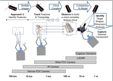
To allow a tracker spacecraft to to identify and estimate the movement of a target spacecraft, we
89
approach this problem as illustrated in Figure1. First, we build up a feature set of points located in
90
three dimensions by triangulation of keypoints on successive images of the target in the “Approach”
91
phase. We then locate the camera relative to the matched points by Perspective-n-Point (PnP) solution
92
during the “Track” phase. By projecting the keypoints into three dimensions, we build up a point
93
cloud of the target over many more images in the “Observe” phase, which can then be matched in
94
shape to a point cloud model, and the pose of the model accurately obtained by three-dimensional
95
keypoint correspondences in the “Identify and Analyze” phase. In the end, the tracker spacecraft with
96
robot arms and end effectors is intended to perform a projected “Capture and Servicing” phase.
Figure 1.Process of Orbit Servicing for Small Satellite
Feature-based vision methods reduce complete images to a set of distinct, reproduceable “features”
98
that are represented by small numerical sequences. We apply ORB (Oriented FAST and Rotated
99
BRIEF) point descriptors for 2-D feature matching with high rotation invariance [27]. We then use
100
structure-from-motion methods to triangulate these points in space.
101
2.1. 3D Reconstruction from Camera 102
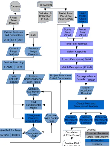
A flowchart of the process we propose is shown in Figure2, with details on each step provided
103
in the following sections. A sequence of images can be captured or cached, features extracted using
104
two-dimensional point descriptors that are stored in memory and matched in pairs to obtain a
105
list of images with features, and also a list of features tracked across images. This list of feature
106
correspondences is used to track the movement of keypoints across several poses, and if the
107
triangulation is not good enough, a more different pose containing those features is selected. Using a
108
pose solution, the points and camera are projected into global coordinates. The resulting scene point
109
cloud can then be compared with a model cloud to identify the target by choosing a set of keypoints
110
and extracting histogram descriptors for each with respect to point normals. By matching descriptors
111
between the scene and model, the model and its pose can be found within the scene.
112
2.2. Keypoint Detection and Matching 113
A method of keypoint detection must be used to obtain keypoints from a sequence of images.
114
The FAST keypoint detector (Features from Accelerated Segment Test) is frequently used for keypoint
115
detection due to its speed, and is used for quickly eliminating unsuitable matches in ORB. Starting
116
with an image patchpof size 31x31, each pixel is compared with a Bresenham circle built 45 degrees at
117
a time byx2n+1=xn2−2y(n)−1. The radius of the surrounding circle of points is nominally 3 points,
118
but is 9 for the ORB descriptor, which expands the patch size and number of points in the descriptor.
119
If at least 75% of the pixels in the circle are contiguous and more than some threshold value above
or below the pixel value, a feature is considered to be present [28]. The ORB algorithm introduces an
121
orientation measure to FAST by computing corner orientation by intensity centroid, defined as
122
C=
m10 m00,
m01 m00
where mpq =
∑
x,yxpyqI(x,y). (1)
The patch orientation can then be found byθ=atan2(m01,m10)and is Gaussian smoothed. ORB 123
then applies the BRIEF feature descriptor fn(p) =∑1≤i≤n2i−1τ(p;ai,bi), a bit string result of binary
124
intensity testsτ, each of which is defined from the intensityp(a)of a point atarelative to the intensity 125
p(b)at a point atbby [28]
126
τ(p;a,b) =
(
1 : p(a)<p(b) 0 : p(a)≥p(b)
)
(2)
The descriptor is also steered according to the orientations computed for the FAST keypoints by
127
rotating the feature set of points(ai,bi)in 2xnmatrix form by the patch orientationθto obtain the 128
rotated setF[27].
129
F=Rf a1
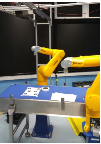
· · · an
b1 · · · bn
!
. (3)
The steered BRIEF operator used in ORB then becomesgn(p,θ) = fn(p)∨(ai,bi)∈F. A lookup
130
table of steered BRIEF patterns is constructed from this to speed up computation of steered descriptors
131
in subsequent points.
132
Keypoints are then matched between two images in the sequence by attempting to find a
133
corresponding keypointa0in the second image that matches each pointain the first image, which can
134
be done exhaustively by anXORoperation between each descriptor and a population count to obtain
135
the Hamming distance. However, The FLANN (Fast Library for Approximate Nearest Neighbor)
136
search algorithm built into OpenCV is used in current work as it performs much faster while still
137
providing good matches [29].
138
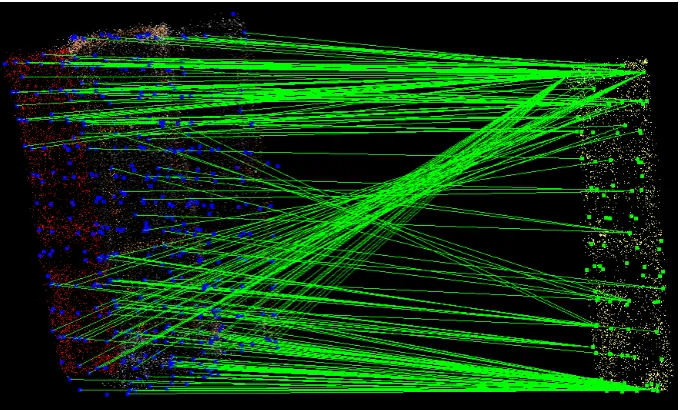
The more features in common between these images, the more potentially good matchesMf can
139
be found, but it is essential that matches be correct correspondences or a valid transformation between
140
the two images will be impossible. The matchesMf are first coarsely pruned of bad pairings by finding
141
the maximum distance between pointsdmaxand then removing all matches that have a coordinate
142
distancedaof more than half the maximum distance between features usingMg= Mf(a)|da<dmax/2.
143
2.3. Three-Dimensional Projection 144
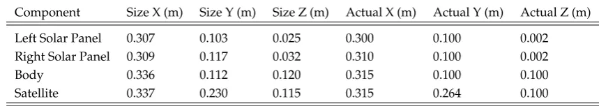
To obtain depth in a 3-D scene, an initial baseline for 3-D projection is first required using either
145
stereoscopic vision, or two sequential images from different angles.. The Fundamental MatrixFis the
146
transformation matrix that maps each point in a first image to a second image, and the set of “good”
147
matchesMgis used where each keypointaiin the first image is expected to map to a corresponding
148
keypointa0i on the epipolar line in the second image by the relation ai0TFai = 0, i = 1, . . . ,n [30].
149
For three-dimensional space, this equation is linear and homogeneous and the matrixF has nine
150
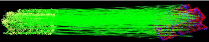
unknown coefficients, soFcan be uniquely solved for by using eight keypoints with the method of
151
Longuet-Higgins [31]. However, due to image noise and distortion, linear least squares estimation (i.e.
152
minF∑i(a0iTFai)2) or RANSAC [32] must be used to ensure that a “best” solution can be estimated. We
153
use RANSAC for its speed to estimateFfor all matchesMgand estimate the associated epipolar lines
154
[33]while removing outliers more than 0.1 from their epipolar line fromMgto yield a final, reliable set
155
of keypoint matchesMh. To perform a projection into un-distorted space, a calibration matrixKis
156
needed, either from calibration with a known pattern such as a checkerboard [34], or estimated for a
157
sizew×himage as
K=
max(w,h) 0 w/2
0 max(w,h) h/2
0 0 1
. (4)
A camera matrix is defined asC=K[R|t]with the rotation matrixRand the translation vector
159
t defining the pose of the camera in space, and for two images, we define two camera matrices
160
C1andC2. To localize a point in un-distorted space, we formulate the so-called essential matrix
161
E = t×R = KTFKthat relates two matching undistorted points ˆx and ˆx0 in the camera plane as
162
ˆ
a0iTEaˆi=0, i=1, . . . ,n[35]. In this way,Eincludes the “essential” assumption of calibrated cameras
163
[36], and is related to the fundamental matrix byE.
164
After calculatingE, we can find the location of a second cameraC2by assuming for simplicity
165
that the first camera is uncalibrated and located at the origin (C1= [I|0]). We decomposeE=t×R 166
into its componentRandtmatrices by using the singular value decomposition ofE[37]. We start with
167
the orthogonal matrixWand and singular value decomposition (SVD) ofE, defined as
168
W=
0 −1 0
1 0 0
0 0 1
SVD(E) =U
1 0 0
0 1 0
0 0 0
V. (5)
The matrixWdoes not directly depend onE, but provides a means of factorization forE. Detailed
169
proofs can be found in [37] and are not reproduced here, but there are two possible factorizations
170
ofR, namelyR=UWTVTandR=UWVT, and two possible choices fort, namelyt= U(0, 0, 1)T
171
andt=−U(0, 0, 1)T. Thus when determining the second camera matrixC2=K[R|t], we have four
172
choices in total.
173
it is now possible to triangulate the original un-distorted point positions in space withEand a pair
174
of matched keypoints[a= (ax,ay),b= (bx,by)]∈Mhusing iterative linear least-squares triangulation
175
[35]. A point in three dimensionsx= (xx,xy,xz, 1)written in the matrix equation formAx=0 results
176
in four linear nonhomogeneous equations in four unknowns for an appropriate choice ofA4x4. To 177
solve this, we can write the system asAx = B, withx = (xx,xy,xz), andA4x3andB4x1as defined 178
by Shil [38]. The solutionxby SVD is transformed to un-distorted space by ˆx = KC1x, assuming
179
that the point is neither at 0 nor at infinity. This triangulation must be performed four times for each
180
combination ofRandtand tested by perspective transformation withC1and ˆxz>0 to ensure the
181
resulting pointspiare in front of the camera.
182
2.4. Image Selection 183
Using adjacent pairs of images in a closely-spaced time sequence allows feature points to be
184
tracked more reliably between images, as there is less chance of conditions or change in angle
185
causing a feature to change significantly. However, the disadvantage of using closely-spaced
186
images for pose estimation is that a very small angular difference between two images will prevent
187
triangulation solutions, like very distant points. Therefore, we track, match, and store keypoints
188
between closely-spaced images, but only triangulate with images that are well-separated that contain
189
tracked keypoints between the two.
190
If two few features are matched between imagePt at time steptandPt−1, the next image to 191
be obtainedPt+1is used withPt−1, if it fails thenPt+2is used, and so on until a predefined “reset” 192
limit. Valid matches from the new imagePtor later are added the the existing tracked keypoint list to
193
associate feature numbers across the sequence of images. When obtaining the fundamental matrixF,
194
only keypoints that have been associated between both images are used.
2.5. Pose Estimation 196
To finding the ego-motion of the tracker’s camera relative to feature points represents the
197
Perspective & Point (PnP) problem. For this, we apply the OpenCV implementation of the EPnP
198
algorithm [39]. For then-point cloud with pointsp1. . .pn, four control pointsci define the world
199
coordinate system and are chosen with one point at the centroid of the point cloud and the rest
200
oriented to form a basis. Each reference point is described in world coordinates (denoted withw)
201
as a linear combination ofciwith weightingsαij. This coordinate system is consistent across linear
202
transforms, so they have the same combination in the camera coordinate system (denoted withc. The
203
known two-dimensional projectionsuiof the reference pointspiare linked to these weightings byK
204
considering that the projection involves scalar projective parameterswi, leading to the following.
205
pwi =
4
∑
j=1
αijcwj , pci =
4
∑
j=1 αijccj,
4
∑
j=1
αij =1 (6)
Kpci =wi ui
1 !
=K 4
∑
j=1
αijccj (7)
The expansion of this equation has 12 unknown control points andnprojective parameters. Two
206
linear equations can be obtained for each reference point to obtain a system of the formMx=0, where
207
the null space or kernel of the matrixM2nx12gives the solutionx= [cc1T,c2cT,cc3T,cc4T]to the system of
208
equations, which can be expressed asx=∑mi=1βivi. The setviis composed of the null eigenvectors
209
of the productMTMcorresponding tomnull singular values ofM. The method of solving for the
210
coefficientsβ1. . .βmdepends on the size ofm, and four different methods are used in the literature
211
[39] for practical solution.
212
Let the translation and rotation in world coordinates of the previous pose be tw(t−1) and
213
Rw(t−1), and that of the current pose betw(t)andRw(t), for which we need to find the current camera
214
matrix in world coordinatesCw(t). The relative transformation between the camera positionst(t)and
215
R(t)is used to incrementally advance the current pose (assumed to be attached rigidly to the camera)
216
asCw(t) = [Rw(t−1)R(t)|R(t) (t(t) +tw(t−1))]., and feature points are incrementally projected
217
into world coordinates withx0 = (Rw(t−1)R(t))Tx+Rw(t−1) (t(t) +tw(t−1)). Orientation is
218
stored as a quaternion from the elementsrijofRw.
219 q= w x y z = √
1+r00+r11+r22
2
r21−r12
2√1+r00+r11+r22 r02−r20
2√1+r00+r11+r22 r10−r01
2√1+r00+r11+r22
(8)
2.6. Object Pose Estimation 220
Object pose estimation focuses on the 3D reconstruction of the object and from the 3D point cloud
221
features are extracted to detect and classify the detect. There are four main segmentation methods:
222
local features [40] [41] [42], global features [43], graph matching [44] and machine learning [45] [46].
223
The use of point clouds in the presence of noise, varying mesh resolutions or poorly textured objects,
224
clutter, and occlusion are very challenging [47] [48]. Segmentation in unstructured environments is
225
difficult [49]. The image data for spacecraft and satellites in orbit are also often distorted and partially
226
occluded due to shadowing. Using 3D point cloud-based recognition methods emphasizes overall
227
shape and configuration over texture and can tolerate a degree of distortion and occlusion. We test the
228
proposed system of using 3D keypoint descriptors by using images of a real satellite model.
229
The PnP solution across a sequence of images allows us to track the pose of the tracker spacecraft
230
relative to features on the target spacecraft. However, in most cases it is necessary to identify what
the actual orientation of the target is with respect to a known geometric model, or to identify specific
232
parts of the target for interaction or analysis. For this task, we use the positional correspondences
233
of three-dimensional keypoints selected from the constructed point cloud with respect to keypoints
234
selected from a reference model point cloud that can be obtained in advance or on-line from another
235
sequence of images with known relative pose. These 3D keypoints (not to be confused with the
236
2D keypoints used for triangulation) provide a means to compare models on a per-pose basis with
237
accumulated points in the scene point cloud once a sufficient number of images has been acquired
238
during the “Observation” phase. This makes it possible to match parts of a structure without requiring
239
the entire structure to have keypoints, for example if the target is in partial shadow. It also allows
240
us to match parts of the target separately given a sufficient number of points in the part that we are
241
matching to.
242
2.7. Target Identification 243
Evidence of a particular pose and instance of the model in the scene is initialized before voting
244
by obtaining the vector between a unique reference point CM and each model feature point FiM 245
and transforming it into local coordinates by the transformation matrixRMGL = [LiM,x,LMi,y,LiM,z]Tfrom
246
the local x-y-zreference frame unit vectors LM
i,x, LiM,y, and LiM,z. This precomputation can be done
247
offline for the model in advance and is performed by calculating for each feature a vectorViM,L =
248
[LM
i,x,LiM,y,LiM,z]·(CM−FiM). For online pose estimation, Hough voting is performed by each scene
249
featureFjSthat has been found by FLANN matching to correspond with a model featureFiM, casting a
250
vote for the position of the reference pointCMin the scene. The transformationRMSLthat makes these
251
points line up can then be transformed into global coordinates with the scene reference frame unit
252
vectors, scene reference pointFS
j and scene feature vectorViS,LasViS,G= [LSj,x,LSj,y,LSj,z]·ViS,L+FjS. The
253
votes cast byViS,Gare thresholded to find the most likely instance of the model in the scene, although
254
multiple peaks in the Hough space are fairly common and can indicate multiple possibilities for model
255
instances. Due to the statistical nature of Hough voting, it is possible to recognize partially-occluded or
256
noisy model instances, though accuracy may be lower. In the case that multiple matches are identified,
257
a criteria for determining which one is the most appropriate is necessary. We choose the match with
258
the largest number of corresponding keypoints as the most likely correct match.
259
2.8. Satellite Component Identification 260
The remote capture of spacecraft is a highly sensitive operation that is carefully planned
261
beforehand to minimize the chance of error. For this reason, an automated grasp planner is not
262
a good fit for orbital capture of a known spacecraft. Rather, the exact point on the spacecraft should be
263
specified beforehand using three-dimensional models, and the grasp planned based on the model and
264
knowledge of the spacecraft’s structure. The grasping operation can then be executed based on the
265
position and motion of the target component. It is also necessary to verify the extents of the component
266
and the whole spacecraft to ensure that no accidental contact is made during the grasping operation,
267
which could cause both target and chaser to spin and separate before the grasp is completed.
268
Satellite components are identified by first preparing exemplar point clouds, such as a model
269
of a solar panel, that can be stored and used for reference by the tracker spacecraft. These model
270
point clouds are then located in the actual reconstructed 3-D scene point cloud created by the tracker
271
spacecraft. We focus on the solar panels as an example of external satellite components that are easy
272
to grasp and manipulate in a rendezvous operation, and the body of the spacecraft that indicates
273
overall positioning. Solar panels may also not remain at a precise angle with respect to the spacecraft
274
body, and therefore must be identified in isolation from the spacecraft body to ensure accuracy. The
275
identification process begins with a set of three-dimensional keypoints being chosen from both the
276
scene and the model by randomly choosing individual points from the cloud separated by a given
277
sampling radiusrk. Normals are calculated for these keypoints relative to nearby points so that each
keypoint has a repeatable orientation. The keypoints are then associated with three-dimensional SHOT
279
point descriptors.
280
SHOT descriptors [41] are calculated by grouping together a set of local histograms over the
281
volumes about the keypoint, where this volume is divided into by angle into 32 spherically-oriented
282
spatial bins. Within a given radiusrdof the keypoint, point counts from the local histograms are
283
binned as a cosine function cos(θi) = nu·nvi of the angleθibetween the point normal within the
284
corresponding part of the structurenvi and the feature point normalnu. This has the beneficial effects
285
of creating a general rotational invariance since angles are relative to local normals, accumulating
286
points into different bins as a result of small differences in relative directions, and creating a coarse
287
partitioning that can be calculated fast with small cardinality [50].
288
Comparing the scene keypoint descriptors with the model keypoint descriptors to find good
289
correspondence matches is done using a FLANN search on ak-dimensional tree (k-d tree) structure,
290
similarly to the matching of image keypoints. Additionally, the BOrder Aware Repeatable Directions
291
algorithm for local reference frame estimation (BOARD) is used to calculate local reference frames for
292
each three-dimensional SHOT descriptor [51] to make them independent of global coordinates for
293
rotation and translation invariance. Once a set of nearest correspondences and local reference frames
294
is found, clustering of correspondences to given cluster sizes set by a parameterrcis performed by
295
pre-computed Hough voting to make recognition of shapes more robust to partial occlusion and clutter
296
[52]. At least a threshold ofnthreshvotes in Hough space is needed to estimate a valid pose.
297
3. Results 298
3.1. 3D Reconstruction and Identification 299
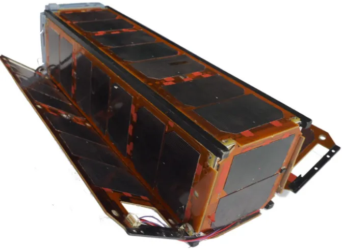
To test the identification of small satellite components, we use an engineering model of a small
300
satellite with full-length fold-out solar panels, shown in Figure3. This satellite serves as an example
301
target for a simulated tracker satellite.
302
Figure 3.Small satellite engineering model
A three-dimensional point cloud of this satellite was created in the laboratory by simulating what
303
a tracker satellite in close proximity would observe as the target tumbles at low relative rotational
304
speed. Rather than rotating the target, the camera was robotically moved at low speed in an arc around
Figure 4.Robot Arm used for positioning camera
Figure 5.Olympus OM-D Camera used for imaging of satellite model
the target satellite in 10 degree increments with the background obscured by a paper screen to prevent
306
unrelated features from being detected and images taken of the target. A high-intensity light source
307
was used to simulate direct sunlight. The robot arm used for motion of the camera is shown in Figure4
308
and the Olympus OM-D E-M1 camera in Figure5. Through 10 complete rotations around the satellite
309
at slightly different angles of view, a sufficiently dense point cloud was triangulated for component
310
recognition. All images were converted to VGA resolution (640x480 pixels) to decrease processing
311
time and demonstrate the feasibility of low-resolution point cloud recognition. Figure6shows the
312
scene as reconstructed by the simulated tracker spacecraft.
313
Using the same process, point clouds were obtained of a solar panel and the satellite body itself.
314
Figure7shows the point clouds generated for these components.
315
3.2. 3D Component Identification 316
Each of the component point clouds shown in Figure7was sequentially matched with the scene
317
of the small satellite in Figure6. To illustrate the matching process, the point cloud matched for each
318
component is marked in yellow with keypoints indicated in green, and the scene is in full colour with
319
keypoints marked in blue. The points of the matched component within the scene are indicated in red
320
to show where the component’s location has been identified.
Figure 6.Scene reconstructed from tracker spacecraft using structure-from-motion
Figure 7.Spacecraft component point clouds: solar panel (left), spacecraft body (right)
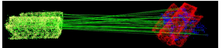
First, the solar panels were matched. Figure8shows the best match for the solar panel model,
322
which corresponds with the left-side solar panel in the scene. Figure9shows a lower-likelihood match,
323
which corresponds to the right-side solar panel in the model. Using the model of the satellite body,
324
Figure10shows the body of the satellite identified.
325
The parameters used for the SHOT descriptors in these tests were a model and scene sampling
326
radius ofrk=0.025m, reference frame and descriptor radius ofrd=0.5m, cluster size ofrc=0.25m,
Figure 8.Matched location (red points) for left solar panel component (yellow points)
Figure 9.Matched location (red points) for right solar panel component (yellow points)
and clustering threshold ofnthresh = 5. The number of correspondences and percentage of error
328
observed in both rotation and translation is shown in Table2. As there are less keypoints in smaller
329
components such as the solar panels, they exhibit higher error in correspondence. Increasing the
330
number of keypoints (and computational time) serves to mitigate this problem.
331
Table 2.Correspondences and Error resulting from varying Descriptor Radius and Cluster Size
Component Corresp
-ondences
Translation Error
Rotation Error
Left Solar Panel 243 3% 5%
Right Solar Panel 186 3% 6%
Spacecraft Body 375 2% 3%
3.3. Dimensional Analysis 332
For each component identified on the spacecraft, we in addition estimate its size for purposes
333
of planning and grasping for the chaser spacecraft. Table3shows the dimensions of the components
334
estimated during the identification process, compared with actual measurements of size. The
335
measurements of size in each direction are performed with respect to the coordinate axes for each
336
component model, and simply indicate the extents of the scene points that have been matched with
337
the model. For the spacecraft considered here, this is suitable since all components are rectangular in
338
form except for the entire satellite as a unit. The detected dimensions of each component are larger
339
than their actual values because the scene points exhibit some degree of statistical variation due to
340
numerical inaccuracies during the triangulation process, and this must be accounted for in planning
341
and control of capture operations as well. This is particularly true for theZaxis measurement of the
342
thin solar panels. The closer and more accurately the chaser spacecraft can observe the target, the
343
smaller these triangulation errors will be, since triangulation error increases with distance..
344
Table 3.Dimensional Analysis of Spacecraft Components
Component Size X (m) Size Y (m) Size Z (m) Actual X (m) Actual Y (m) Actual Z (m)
Left Solar Panel 0.307 0.103 0.025 0.300 0.100 0.002
Right Solar Panel 0.309 0.117 0.032 0.310 0.100 0.002
Body 0.336 0.112 0.120 0.315 0.100 0.100
Satellite 0.337 0.230 0.115 0.315 0.264 0.100
3.4. Parameter Effects on Spacecraft Pose Identification Accuracy 345
To illustrate the accuracy of pose estimation while varying the descriptor radiusrdand cluster size
346
rcand therefore processing times, a set of pose estimation tests were performed. These tests use a point
347
cloud of the complete spacecraft that was generated from a different series of images so that a different
348
point cloud with the same shape could be matched against the scene. In three examples of target
349
identification shown in Figure11, Figure12, and Figure13, high-density model points are in yellow
350
with selected keypoints in green, and low-density scene keypoints are shown in blue. The model
351
instance found in the scene is overlaid in red from a high-density model composed of 26339 points,
352
while the scene is composed of 1960 points triangulated from 52 images. The number of keypoints was
353
reduced by radius to 2042 in the model and 1753 in the scene.
Figure 11.Pose Correspondence for Estimate 1, Descriptor Radius 0.5m, Cluster Size 0.25m
Figure 12.Pose Correspondence for Estimate 1, Descriptor Radius 0.5m, Cluster Size 0.025m
Figure 13.Pose Correspondence for Estimate 1, Descriptor Radius 0.125m, Cluster Size 0.25m
The descriptor radius and cluster size for these estimates, with the resulting number of
355
correspondences and rounded cumulative errors in translation and rotation are shown in Table
356
4.
357
Table 4.Correspondences and Error resulting from varying Descriptor Radius and Cluster Size
Estimate Descr. Radius (m)
Cluster Size (m)
Corresp -ondences
Translation Error
Rotation Error
1 0.5 0.25 507 1% 2%
2 0.5 0.025 507 7% 3%
3 0.125 0.25 45 3% 4%
As more scene points are added over time, accuracy can increase, but only if they are consistent
358
with the existing scene. We can see from these results that increasing the size of the SHOT descriptor
359
will increase the number of keypoints available and result in better accuracy and higher likelihood
360
of identifying a shape, but also will require longer processing times. Cluster sizes must be set
361
appropriately for the point cloud size, as a cluster size too small or too large will prevent valid
362
instances from being found, and result in decreased accuracy.
363
The patent-free ORB algorithm that combines FAST keypoint detection and BRIEF feature
364
descriptors provides good tolerance to rotation and scaling of features for this purpose. For useful
365
reconstruction, it is important to identify as many features as possible, so target spacecraft with
many colors, edges, and shapes generally provide the best results for feature-based systems such as
367
this. It is important to note that this method of motion estimation provides best solutions through
368
post-processing of results. The more images that are included when creating the structure, the better
369
triangulation will be. If processing power and storage is available to include a large number of recent
370
images, such as by observing the target through multiple rotations, a better solution for motion will be
371
obtained. To additionally decrease the processing time if desired, the camera image can be lowered in
372
resolution, or pixels can be under-sampled by choosing only every 2nd pixel or every 4th pixel in a
373
staggered pattern over the image for feature matching [53].
374
3.5. Occlusion Effects on Spacecraft Pose Identification Accuracy 375
In the space environment, it is common that components are partially or fully occluded by
376
shadows, which can be cast by either the chaser spacecraft or other components of the target spacecraft.
377
These shadows are total in an airless environment and prevent any features from being detected
378
in a shadowed scene. To evaluate the effects of partial shadowing on the small spacecraft model,
379
features were removed from the scene point cloud used in previous tests so that along the length of the
380
spacecraft, the first 25%, 50%, and then 75% of features are in shadow, as shown in Figure14, Figure
381
15, and Figure16respectively. All tests use a descriptor radiusrd=0.5mand a cluster Sizerc=0.25m.
382
Figure 14.Pose Correspondence for 25% of the scene in shadow
Figure 15.Pose Correspondence for 50% of the scene in shadow
Figure 16.Pose Correspondence for 75% of the scene in shadow
The effects of this occlusion on the model-to-scene correspondence and pose estimation accuracy
383
are summarized in Table5. A small amount of shadow over a quarter of the scene has a tolerable
384
but noticeable effect on both translation and rotation estimation. However, with half of the target
385
shadowed, translation error increases in a linear fashion while rotation error increases much more
quickly due to the high sensitivity of rotation estimation to the observed point cloud shapes in the
387
scene. With three-quarters of the target in shadow, no pose estimate can be found as the scene point
388
cloud no longer bears a similar enough shape to the model.
389
Table 5.Correspondences and Error resulting from varying Descriptor Radius and Cluster Size
Percent Shadowed
Translation Error
Rotation Error
25% 4% 8%
50% 8% 21%
75% No Pose No Pose
3.6. Timing and Profiling 390
To profile the processing requirements of the described algorithms on a system that could
391
potentially be embedded into a satellite, the algorithm was run on a 667MHzARM Cortex-A9 processor
392
over the VGA images of the satellite engineering model used above, and raw timing statistics gathered
393
for the processing time of each algorithm. Tests 1 and 2 were performed with 6524 model points and
394
5584 scene points from 220 images, and tests 3 and 4 were performed with 6524 model points and
395
1816 scene points from 32 images. Tests 1 and 3 were performed with a descriptor radius of 0.05 and
396
cluster size of 0.1, and Tests 2 and 4 were performed with a descriptor radius of 0.1 and cluster size of
397
0.5. Table6and Table7show the timing information obtained in seconds for each of the described
398
algorithms in these cases. While accurate matching of large models and scenes can take on the order of
399
minutes, this does not prevent a chaser spacecraft from building a motion model over long periods of
400
time from stored images before acting to rendezvous, and both software and hardware acceleration
401
methods may be used to further improve this performance.
402
Table 6.Timing for Features, Triangulation and PnP in seconds
Test Num.
Feature Detect.
Feature Matching
Feature Selection
Fundam. Matrix
Essential Matrix
Triangu -lation
PnP RANSAC
Ego-Motion
Total Time
1-2 0.12 0.058 0.015 0.083 0.0017 0.038 0.0033 0.0005 0.32
3-4 0.12 0.061 0.010 0.048 0.0014 0.025 0.0026 0.0004 0.27
Table 7.Timing for Correspondence and Identification in seconds
Test Num.
Model Normals
Scene Normals
Model Sampling
Scene Sampling
Model Keypoints
Scene Keypoints
FLANN Search
Clustering Total Time
1 0.17 0.15 0.027 0.020 1.26 0.84 107.7 0.92 112.1
2 0.17 0.15 0.029 0.024 3.37 2.19 118.0 2.00 127.2
3 0.17 0.043 0.031 0.0083 3.31 0.37 42.5 0.63 48.4
4. Conclusions 403
This study proposes a 3D pose estimation, recognition and identification system for a small
404
spacecraft servicing mission that uses a monocular camera sensor. This study uses Structure from
405
Motion (SFM) to build 3D model from 2D images and a SHOT descriptor to identify surface shape
406
components. The EPnP process estimates object poses and increases the system’s ability to identify
407
position and angles. The experimental results show that the proposed system can effectively identify
408
components and poses of a spacecraft model in the lab. Potential application of this system to an
409
orbital demonstration mission with industry partners is under investigation.
410
In this work, we have described a feature-based visual identification system that allows a tracker
411
spacecraft to track relative movement to a target and ultimately acquire pose estimates using point
412
cloud techniques. Using projective geometry, we perform three-dimensional reconstruction of features
413
on the target from a sequence of images taken with a single camera. It is intended that even small
414
spacecraft with a single camera could take advantage of this system. Work is underway to scale this
415
system to a level suitable for small satellite use, which could provide a technology demonstration
416
with a minimum of cost and risk. As the performance of feature tracking depends very heavily on the
417
design of the feature descriptor and method of matching, further comparison of descriptor types for
418
both two-dimensional and three-dimensional matching is warranted, and FPGA acceleration is being
419
developed for this system. Future work also includes the validation of these methods with a variety of
420
different spacecraft and vision hardware, and under a broader set of varying conditions to evaluate
421
the robustness of feature-based systems.
422
Author Contributions:All authors contributed equally to this manuscript. Dr Post is the principal author of this 423
manuscript and is responsible for programming and experimental testing. Dr Li contributed background research 424
and analysis of the results. Both are responsible for the writing of the manuscript. 425
Conflicts of Interest:The authors declare no conflict of interest. 426
References 427
1. Ruel, S.; Luu, T.; Berube, A. Space shuttle testing of the TriDAR 3D rendezvous and docking sensor. Journal 428
of Field Robotics2012,29, 535–553. 429
2. Hinkel, H.; Cryan, S.; DSouza, C.; Strube, M. NASA’s Automated Rendezvous and Docking/Capture 430
Sensor Development and Its Applicability to the GER.NASA Report2014. 431
3. Padial, J.; Hammond, M.; Augenstein, S.; Rock, S.M. Tumbling target reconstruction and pose estimation 432
through fusion of monocular vision and sparse-pattern range data. Multisensor Fusion and Integration for 433
Intelligent Systems (MFI), 2012 IEEE Conference on. IEEE, 2012, pp. 419–425. 434
4. Oda, M. Experiences and lessons learned from the ETS-VII robot satellite. Robotics and Automation, 2000. 435
Proceedings. ICRA’00. IEEE International Conference on. IEEE, 2000, Vol. 1, pp. 914–919. 436
5. Ruth, M.; Tracy, C. Video-guidance design for the DART rendezvous mission. Defense and Security. 437
International Society for Optics and Photonics, 2004, pp. 92–106. 438
6. Zhang, H.; Jiang, Z.; Elgammal, A. Satellite recognition and pose estimation using homeomorphic manifold 439
analysis. IEEE Transctions on Aerospace and Electronic Systems2015,51, 785–793. 440
7. Sharma, S. Pose Estimation of Uncooperative Spacecraft using Monocular Vision. Stanford’s 2014 PNT 441
Challenges and Opportunities Symposium, Kavli Auditorium, SLAC, 2014. 442
8. Tzschichholz, T.; Boge, T.; Benninghoff, H. A flexible image processing framework for vision-based 443
navigation using monocular imaging sensors. Proceedings of the 8th international ESA conference on 444
guidance, navigation & control systems. Karlovy Vary, Czech Republic, 2011. 445
9. Tweddle, B.E.; Setterfield, T.P.; Saenz-Otero, A.; Miller, D.W.; Leonard, J.J. Experimental evaluation of 446
on-board, visual mapping of an object spinning in micro-gravity aboard the International Space Station. 447
Intelligent Robots and Systems (IROS 2014), 2014 IEEE/RSJ International Conference on. IEEE, 2014, pp. 448
2333–2340. 449
10. Aghili, F.; Kuryllo, M.; Okouneva, G.; English, C. Fault-tolerant position/attitude estimation of free-floating 450
11. Flores-Abad, A.; Ma, O.; Pham, K.; Ulrich, S. A review of space robotics technologies for on-orbit servicing. 452
Progress in Aerospace Sciences2014,68, 1 – 26. 453
12. Post, M.A.; Yan, X.T.; Li, J.; Clark, C. Visual Pose Estimation System for Autonomous Rendezvous of 454
Spacecraft. 13th Symposium on Advanced Space Technologies in Robotics and Automation (ASTRA 2015) 455
- Noordwijk, Netherlands, 2015, pp. 1–9. 456
13. Zhang, H.; Wei, Q.; Jiang, Z. 3D reconstruction of space objects from multi-Views by a visible sensor. 457
Sensors2017,7, 1 – 16. 458
14. Depeuter, W.; Visentin, G.; Fehse, W. Satellite servicing in GEO byrobotic service vehicle. ESA 459
Bulletin-European Space Agency1994,7, 22 – 25. 460
15. Hirzinger, G.; Landzettel, K.; Brunner, B.; Fischer, M.; Preusche, C.; Reintsema, D.; Albu-Schäffer, A.; 461
Schreiber, G.; Steinmetz, B.M. DLR’s robotics technologies for on-orbit servicing.Advanced Robotics2004, 462
18, 139 – 174. 463
16. B, B.; Kerstein, L. ROGER-robotic Geostationary Orbit Restorer. 54th International Astronautical Congress 464
of the International Astronautical Federation, Bremen, Germany, 2003. 465
17. Kaisera, C.; Sjöbergb, F.; Delcurac, J.M.; Eilertsen, B. SMART-OLEV an orbital life extension vehicle for 466
servicing commerial spacecrafts in GEO.Acta Astronautica2008,63, 400 – 410. 467
18. Rupp, T.; Boge, T.; Kiehling, R.; Sellmaier, F. Flight Dynmacis Challenges of Germanon-Orbit Servicing 468
Mission. International Symposium on Space Flight Dynamics Toulouse France September 27- October 2, 469
2009. 470
19. Kimura, S.; Nagai, Y.; Yamamoto, H.; Masuda, K.; Abe, N. Approach for on Orbit Maintenance and 471
Experiment Plan using 150kg Class Satellites. IEEE Aerospace Conference Big Sky USA March 5-12, 2005. 472
20. Richards, R.; Tripp, J.; Pashin, S.; King, D.; Bolger, J.; Nimelman, M. Advances in Automous Orbital 473
Rendezvous Technology: The XSS-11 Lidar Sensor. Proceedings of the 57th IAC/IAF/IAA (International 474
Astronautical Congress) Valencia Spain October 2-6, 2005. 475
21. Thienel, J.K.; Sanner, R.M. Hubble space telescope angular velocity esitmatin during the robotic servicing 476
mission.Journal of Guidance Control and Dynamics2007,30, 29 – 34. 477
22. Nishida, S.I.; Kawamoto, S.; Okawa, Y.; Terui, F.; Kitamura, S. Space debris removal system using a small 478
satellite. Acta Astronautica2009,65, 95 – 102. 479
23. Thomas, D.; Sean, D. Overview and Performance of the Front-end Robotics Enabling Near-term 480
Demonstration. AIAA Infotech Aerospace Conference Seattle USA April 6-9, 2009. 481
24. Rekleitis, I.; Martin, E.; Rouleau, G.; L’Archevêque, R.; Parsa, K.; Dupuis, E. Autonomous capture of a 482
tumbling satellite. Journal of Field Robotics2007,24, 275 – 296. 483
25. Roesler, G. Robotic Servicing of Geosynchronous Satellites DARPA. Online, 2016. 484
26. Goldberg, S.B.; Maimone, M.W.; Matthies, L. Stereo vision and rover navigation software for planetary 485
exploration. Aerospace Conference Proceedings, 2002. IEEE. IEEE, 2002, Vol. 5, pp. 5–2025. 486
27. Rublee, E.; Rabaud, V.; Konolige, K.; Bradski, G.R. ORB: An efficient alternative to SIFT or SURF. ICCV 487
2011, 2011, pp. 2564–2571. 488
28. Rosten, E.; Drummond, T. Fusing points and lines for high performance tracking. Computer Vision, 2005. 489
ICCV 2005. Tenth IEEE International Conference on, 2005, Vol. 2, pp. 1508–1515. 490
29. Muja, M.; Lowe, D.G. Fast Approximate Nearest Neighbors with Automatic Algorithm Configuration. 491
International Conference on Computer Vision Theory and Application (VISSAPP’09). INSTICC Press, 2009, 492
pp. 331–340. 493
30. Luong, Q.T.; Faugeras, O. The Fundamental matrix: theory, algorithms, and stability analysis. International 494
Journal of Computer Vision1995,17, 43–75. 495
31. Longuet-Higgins, H.C. A computer algorithm for reconstructing a scene from two projections. InReadings 496
in computer vision: issues, problems, principles, and paradigms; Fischler, M.A.; Firschein, O., Eds.; Morgan 497
Kaufmann Publishers Inc.: San Francisco, CA, USA, 1987; pp. 61–62. 498
32. Fischler, M.A.; Bolles, R.C. Random sample consensus: a paradigm for model fitting with applications to 499
image analysis and automated cartography. Commun. ACM1981,24, 381–395. 500
33. Feng, C.L.; Hung, Y.S. A Robust Method for Estimating the Fundamental Matrix. In International 501
Conference on Digital Image Computing, 2003, pp. 633–642. 502
34. Hartley, R. Self-Calibration of Stationary Cameras. International Journal of Computer Vision1997,22, 5–23. 503
36. Shil, R. Structure from Motion and 3D reconstruction on the easy in OpenCV 2.3+. Online, 2012. 505
37. Hartley, R.I.; Zisserman, A.Multiple View Geometry in Computer Vision, second ed.; Cambridge University 506
Press, ISBN: 0521540518, 2004. 507
38. Shil, R. Simple triangulation with OpenCV from Harley & Zisserman. Online, 2012. 508
39. Moreno-Noguer, F.; Lepetit, V.; Fua, P. Accurate Non-Iterative O(n) Solution to the PnP Problem. IEEE 509
International Conference on Computer Vision Rio de Janeiro, Brazil, 2007. 510
40. Johnson, A.E.; Hebert, M. Using spin images for efficient object recognition in cluttered 3D scenes. IEEE 511
Transctions on Pattern Analysis and Machine Intelligence1999,21, 433 – 449. 512
41. Tombari, F.; Salti, S.; Stefano, I.D. Unique Signatures of Histograms for Local Surface Description. European 513
Conference on Computer Vision, Springer Berlin Heidelberg, 2010, pp. 356–369. 514
42. Rusu, R.B.; Blodow, N.; Beetz, M. Fast Point Feature Histograms for 3D Registration. IEEE Robotics and 515
Automation Conference ICRA Kobe May 12-17, 2009, pp. 3212–3217. 516
43. Rusu, R.B.; Blodow, N.; Beetz, M. Fast 3d Recognition and Pose using the Viewpoint Feature Histogram. 517
IEEE/RSJ Internaltional Conference on Intelligent Robots and Systems, 2010, pp. 2155–2162. 518
44. Hao, W.; Wang, Y. Structure-based object detection from scene point clouds. Neurocomputing2016,191, 148 519
– 160. 520
45. Wang, Z.; Zhang, L.; Fang, T.; Mathiopoulos, P.T.; Tong, X.; Qu, H.; Xiao, Z.; Li, F.; Chen, D. A multiscale 521
and hierachical feature extraction method for terrestrial laser scanning point cloud classification. IEEE 522
Transactions on Geoscience and Remote Sensing2014,53, 2409 – 2425. 523
46. Chen, J.; Fang, Y.; Cho, Y.K. Performance evaluation of 3D descriptors for object recognition in construction 524
applications. Automation in Construction2018,86, 44 – 52. 525
47. Yang, J.; Zhang, Q.; Xiao, Y.; Cao, Z. TOLDI: An effective and robust approach for 3D local shape description. 526
Pattern Recognition2017,65, 175 – 187. 527
48. Wohlhart, P.; Lepetit, V. Learning Descriptors for Object Recognition and 3D Pose Estimation. CoRR2015, 528
abs/1502.05908. 529
49. Choi, C.; Christensen, H.I. RGB-D object pose estimation in unstructured environments. Robotics and 530
Autonomous Systems2016,75, 595 – 613. 531
50. Salti, S.; Tombari, F.; Di Stefano, L. SHOT: unique signatures of histograms for surface and texture 532
description. Computer Vision and Image Understanding2014,125, 251–264. 533
51. Petrelli, A.; Di Stefano, L. On the repeatability of the local reference frame for partial shape matching. 534
Computer Vision (ICCV), 2011 IEEE International Conference on. IEEE, 2011, pp. 2244–2251. 535
52. Tombari, F.; Di Stefano, L. Object recognition in 3D scenes with occlusions and clutter by Hough voting. 536
Image and Video Technology (PSIVT), 2010 Fourth Pacific-Rim Symposium on. IEEE, 2010, pp. 349–355. 537
53. Ambrosch, K.; Zinner, C.; Kubinger, W. Algorithmic Considerations for Real-Time Stereo Vision 538