Different Deterioration Rates Two Storage
Facilities Deteriorating Items Inventory Model
under Time and Price Dependent Demand for
Single Buyer Single Vendor
R.D. Patel, Jiten PatelAbstract— An optimal policy for vendor and buyer is developed for items having deterioration and demand is linear function of time and
price. One vendor and one buyer system model is constructed as profit maximization to determine the system’s optimal cycle time (strategy) under two storage facilities for buyer. We also determine the profit of buyer-vendor jointly. Numerical illustrations show that both buyer and vendor earn significant profit in supply chain inventory system. For parameters, post-optimality analysis is also done.
Index Terms— Two storage facility, Supply chain, Optimal strategy, Different Deterioration, Time dependent demand, price dependent
demand, Time varying holding cost .
—————————— ——————————
1 I
NTRODUCTIONRETAILERS purchase more units than their capacity of Own Warehouse (OW) for getting advantage of price discounts. Additional better storage facility with higher inventory storage cost known as Rented Warehouse (RW) is made for storing excess goods. A two facility location inventory model was first developed by Hartley [1976]. Two facilities location deteriorating items inventory model was obtained by Sarma (1987). A two facilities location deteriorating items inventory model was considered by Benkherouf (1997). Ghosh and Chakrabarty (2007) gave two storage facilities deteriorating items inventory model. Two warehouses inventory model under exponentially decreasing demand was developed by Shah and Munshi (2010). A selling price and advertisement dependent model for two storage location was given by Bhunia et al. (2011). A time dependent demand and variable holding cost inventory model was proposed by Tyagi and Singh (2013). Sheikh and Patel [2017] obtained two facilities location inventory model under varying deterioration. To fulfill customers‘ (buyers‘) demand, many stages either directly or indirectly involves in supply chain. It includes suppliers, manufacturers, transporters, warehouses, retailers, customers, etc. To satisfy demand of customers‘ is the main issue in today‘s situation. For supply chain, there must be need of significant information sharing between buyer and vendor. Better collaboration between buyer and vendor also reduces total cost of supply chain. In past researchers have developed joint buyer vendor inventory system with different assumptions on demand pattern such as price-dependent, time dependent demand, etc. A combined inventory model when vendor has finite production rate for one buyer one vendor has been derived by Banerjee (1986). By considering items having deterioration
---
R.D. Patel, Professor, Department of Statistics, Veer Narmad South Gujarat University, Surat-395007, Gujarat, India
Jiten Patel, Research Scholar, Department of Statistics, Veer Narmad South Gujarat University, Surat-395007, Gujarat, India
2
N
OTATIONS AND ASSUMPTIONS2.1 Notations:
Here notations considered for developing model are: D( t ) : a + b t – ρp, where a > 0, 0 < b< 1, p > 0, ρ > 0 HC(OW) : OW has time varying holding cost (x1 + y1 t, x1 > 0, 0 < y1 < 1)
HC( RW): RW has time varying holding cost (x2+y2t, x2>0,
0<y2<1)
I0b(t) : OW stock size of buyer
Irb(t) : RW stock size of buyer
Iv(t) : Vendor‘s inventory size at time t
Ab : Buyer‘s per order ordering cost
Av : Vendor‘s per order ordering cost
cb : Per unit cost of purchasing of buyer
θ : OW rate of deterioration during t1 < t < t2, 0< θ < 1
θt : OW rate of deterioration during t2 ≤ t ≤ Tb, 0 < θ < 1
xb1 : Fixed holding cost in OW of buyer
yb1 : Buyer‘s varying holding cost in OW
xb2 : RW fixed holding cost of buyer
yb2 : Varying holding cost in RW of buyer
xv : Fixed storage cost of vendor
yv : Varying storage cost of vendor
p : Unit selling price of buyer (a decision variable) m : Preservation technology cost for vendor (fixed) n : Number of time orders placed by buyer during cycle time
tr : When level of inventory of buyer in RW becomes nil
(a decision variable)
W : Capacity of own warehouse of buyer
Assumpltions
The following assumptions are considered for the development of model.
Demand of item is function of price and time. One vendor one buyer are considered. Stock out is not permitted.
Lead time is zero.
During the cycle time, no repairing or replacement of deteriorated units and deterioration is dependent on time for buyer‘s inventory.
For buyer and vendor both, time varying holding cost is considered.
W units fixed capacity in OW and unlimited capacity in RW are considered.
First RW goods are consumed and then goods in OW are consumed.
Unit inventory cost in OW is less than unit inventory cost in RW.
3 THE MODELING AND ANALYSIS
Figure below shows inventory level Ib(t) of buyer at time t
(0 ≤ t ≤ Tb). Buyer’s Inventory
Figure 1
Differential equations in RW and OW of inventory level at time t are expressed as:
r b
d I ( t )
= - ( a + b t - p ) ,
d t
0 t tr (1)
0 b
d I ( t )
= 0 ,
d t r
0 t t (2)
0 b
d I ( t )
= - ( a + b t - p ) ,
d t
tr t t1 (3)
0 b
0 b
d I ( t )
+ θ I (t ) = - (a + b t - p ),
d t
t1 t t2 (4)
0 b
0 b
d I ( t )
+ t I ( t ) = - ( a + b t - p ) ,
d t
t2 t Tb (5)
v
d I ( t )
= - ( a + b t - p ) ,
d t
0 t T (6)
initial conditions taken are I0b(0) = W, I0b(t1) = S1, I0b(tr) = W,
Ir(0) = Q-W, Irb(tr) = 0, I0b(Tb)=0 and Iv(T)=0.
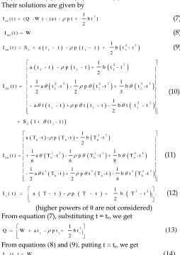
Their solutions are given by 2 r b
1
I ( t ) = ( Q - W ) - ( a t - + b t
2
p t )
(7)
0 b
I (t ) = W (8)
2
0 b 1 1 1
1
I ( t ) = S + a t - t - p t - t + b t - t
2 2 1
(9)
2
1 1
0
2 2 3
1 1
1 1
b
2
1
a t - t - t - t + b t - t
2
1 1 1
+ a t - t - t - t + b t - t
2 2 3
1
- a t t - t + t t - t - b t t - t
2 p
I ( t ) = p
+ S 1 +
p - t ) ( t
2 1
2 2 3
1 1 1
2 1
(10)
2 2
b b b
3 3 3 3 4 4
0 b b b b
2 2 2 2 2
b b b
1
a T - t - T - t + b T - t
2
1 1 1
I ( t ) = + a T - t - T - t + b T - t
6 6 8
1 1 1
- a t T - t + t T - t - b t T - t
2 2 4
p
p
p
(11)
2 2
v
1
I ( t ) = a T - t - p T - t + b T - t .
2
(12)
(higher powers of θ are not considered) From equation (7), substituting t = tr, we get
2
r p tr r
1
Q = W + a t - + b t
2
(13)
From equations (8) and (9), putting t = tr, we get
0 b r
2
0 b r 1 1 r 1 r r
1
I ( t ) = S + a t - t - t - t + b t - t
2
p 12
(15)
So from equations (14) and (15), we have
2
1 - 1 r p 1 r r
1
S = W a t - t + t - t - b t - t
2 2 1
(16)
From equations (10) and (11), putting t = t2, we get
2 21 2 1 2 1 2
2 2 2 2
1 2 1 2
0 b 2
3 3
1 2 2 1 2
2 2
2 1 2 2 1 2
1 1 2
1
a t - t - p t - t + a t - t
2
1 1
- p t - t + b t - t
2 2
I ( t ) =
1
+ b t - t - a t t - t
3
1
+ p t t - t - b t t - t
2
+ S 1 + t - t
(17)
2 2b 2 b 2 b 2
3 3 3 3
b 2 b 2
0 b 2
4 4 2
b 2 2 b 2
2 2 2 2
2 b 2 2 b 2
1
a T - t - p T - t + b T - t
2
1 1
+ a T - t - p T - t
6 6
I ( t ) = .
1 1
+ b T - t - a t T - t
8 2
1 1
+ p t T - t - b t T - t
2 4 (18)
So from equations (17) and (18), we have
2 2 2 2 2 2 2 22 2 2 3
2 2 1 2
3 2 4
2 2 2
4 2
2 2
1 r 2
2
r 1 r 1 r
2 2 2
1 1
2 2 2 2
r
2
1 r 2
b
1
2 a - a θμ
4 b θt a t - 8 a b θt t
+ 8 a b θt t - 4 b θ t a t t - 4 b θt a t
- 4 b θ t W t + 4 b θ t a t - 4 b θ t a t
+ 4 b θ t a t - 4 a θt t + a θ t
- 8 a b t + 8 a b t + 8 a b t - 2 b θt 1
T =
b θμ - 2 + + 8 a b θt 2
2
2 2
1
2 2 2
1 2
3 2 2 2
2 1 2
3 3 2
2 21
3 2 3
2 2
2 2
2
2
r 1 2
2 2
2 2 r
2 2
r
2 2 2
2 2 r
t + 4 b t + 4 a + 8 b W
- 4 b t + 8 b W θt - 8 b W θt - 8 a b θt
+ 4 b θt t - 4 b θt t - 4 b W θt
+ 2 b θt t - 2 b θt t
+ 4 b W θ t - 2 b θ t t
+ 2 b θ t t - 4 a b θt
(19)
Equation (19) states that W and tr expresses Tb and hence Tb is
not a decision variable. Total profit consists of: Buyer’s relevant costs:
(i) Ordering cost (OCb) = n Ab (20)
(ii)
r 1 r b 2 1 2 t t
1 b 1 b 0 b 1 b 1 b 0 b
0 t
b t T
1 b 1 b 0 b 1 b 1 b 0 b
t t
x + y t I ( t ) d t + x + y t I ( t ) d t
H C O W = n
+ x + y t I ( t ) d t + x + y t I ( t ) d t
(21)
(iii)
r t
b 2 b 2 b r b
0
H C R W = n x + y t I ( t ) d t
(22) (iv) b 2 1 2 T t
b b 0 b 0 b
t t
D C = n c I ( t ) d t + t I ( t ) d t
(23)
(v) Sales Revenue:
T b
b
0
S R = n p ( a + b t - p ) d t
2
b b b
1
= n p a T - p T + b T
2
(24)
(by not considering higher powers of θ) (vi) Total Profit
b b b b b b
1
T P = S R - O C - H C ( R W ) - H C ( O W ) - D C
T
(25) Relevant costs of vendor:
(i) Cost of Ordering (OCv) = Av (26)
(ii) Cost of Holding:
b
b T T
v v v b
0 0
T T
v v b
0 0
H C = x I ( t ) d t - n I ( t ) d t
+ y t I ( t ) d t - n t I ( t ) d t
r r 1 2 r 1 b 2 t tr b 0 b
0 0
t t
T
v v 0 b 0 b
0 t t
T
0 b t
I ( t ) d t + I ( t ) d t
= x I ( t ) d t - n + I ( t ) d t + I ( t ) d t
+ I ( t ) d t
r r 1 2 r 1 b 2 t t
r b 0 b
0 0
t t
T
v v 0 b 0 b
0 t t
T
0 b t
t I ( t ) d t + t I ( t ) d t
+ y t I ( t ) d t - n + t I ( t ) d t + t I ( t ) d t
+ t I ( t ) d t
(27) (iii) Preservation Technology Cost (PTCv) = m (28)
(iv) Sales Revenue:
T
2
v b b
0
1
S R = c ( a + b t - p ) d t = c a T - p T + b T
2 (29) (v) Total Profit:
v v v v v
1
T P = S R - O C - H C - P T C
T (30)
b r b r
r
T P (t , p ) T P (t , p )
= 0 , = 0 ,
t p
(31) where b
T T =
n and Tb is function of tr,
provided it satisfies the second order condition
2 2
b r b r
2
2 2
b r b r
2
T P ( t ,p ) T P ( t ,p )
t p T
> 0
T P ( t ,p ) T P ( t ,p )
T p p
(32)
This solution (n, T) maximizes TPv.
Then the total profit without collaboration is given by: TP = max(TPb + TPv).
Situation-II: Joint decision of vendor and buyer: Here buyer and vendor jointly make decision:
For maximum total profit (TP) when buyer and vendor take joint decision, it must fulfil the condition
r r
r
T P (t , p ) T P (t , p )
= 0 , = 0 ,
t p
(33)
for ( b
T T =
n ) is a function of tr,
provided it satisfies the second order condition
2 2
r r
2
2 2
r r
2
T P ( t ,p ) T P ( t ,p )
t p T
> 0
T P ( t ,p ) T P ( t ,p )
T p p
(34)
where total profit (TP) with collaboration is given by:
TP =TPb + TPv (35)
4 NUMERICAL EXAMPLE
Various parameter values in appropriate units are taken for numerical illustration, Ab= 150, W = 135, a = 1200,
b=0.05, cb= 40, θ=0.05, xb1 = Rs. 4, yb1=0.04, xb2 = Rs. 6, yb2=0.08,
Av = 2000, xv = 3, yv=0.03, m = 5, v1=0.30, v2 = 0.50. Table
provides the independent and joint optimal values of tr, T and
profits for buyer and vendor.
Table-1 The optimal solution for without collaboration and with collaboration
Independent Decision Joint Decision
n 5 4
tr 0.0746 0.1582
P 75.4108 56.2746
T 1.4997 1.3484
Buyer‘s Profit 44076.6760 41111.8702
Vendor‘s
Profit 21453.2693 27363.0836
Total Profit 65529.9453 68474.9539
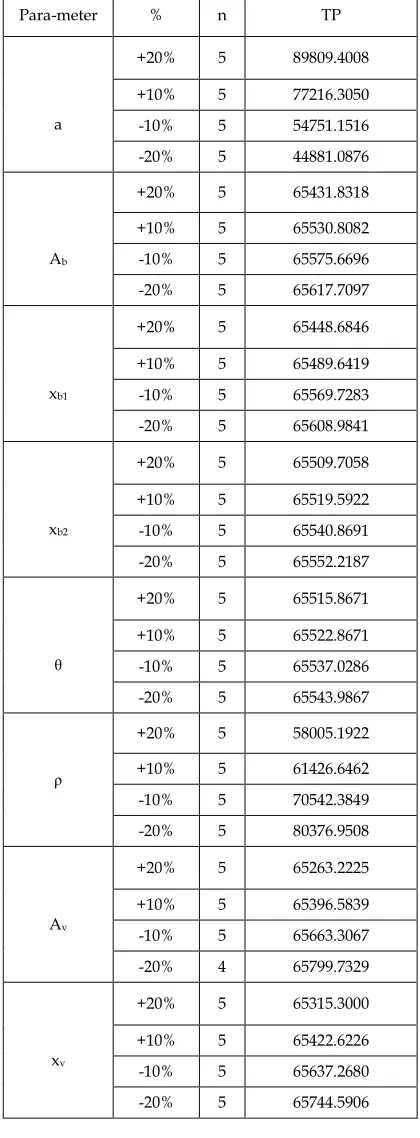
5 POST-OPTIMALITY ANALYSIS
Study of one parameter at a time, post-optimality results of above illustration is done here.
Table 2 Post-optimality Analysis Independent Decision
Para-meter % n TP
a
+20% 5 89809.4008
+10% 5 77216.3050
-10% 5 54751.1516
-20% 5 44881.0876
Ab
+20% 5 65431.8318
+10% 5 65530.8082
-10% 5 65575.6696
-20% 5 65617.7097
xb1
+20% 5 65448.6846
+10% 5 65489.6419
-10% 5 65569.7283
-20% 5 65608.9841
xb2
+20% 5 65509.7058
+10% 5 65519.5922
-10% 5 65540.8691
-20% 5 65552.2187
θ
+20% 5 65515.8671
+10% 5 65522.8671
-10% 5 65537.0286
-20% 5 65543.9867
ρ
+20% 5 58005.1922
+10% 5 61426.6462
-10% 5 70542.3849
-20% 5 80376.9508
Av
+20% 5 65263.2225
+10% 5 65396.5839
-10% 5 65663.3067
-20% 4 65799.7329
xv
+20% 5 65315.3000
+10% 5 65422.6226
-10% 5 65637.2680
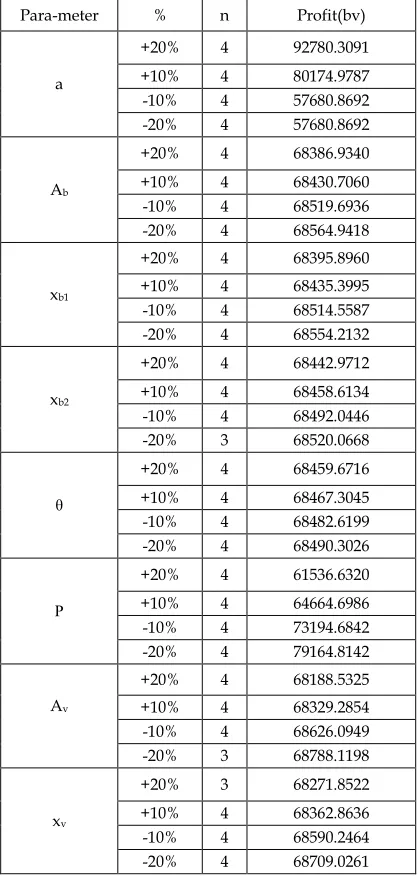
Table 3 Post-optimality Analysis Joint Decision
From Table 2 and 3 computations we observe about variations of optimal cycle time T* and maximum total profits for independent as well as joint decisions. For independent as well as jointly, there will be increase or decrease in value of parameter ‗a‘ when parameter ‗a‘ increase/ decrease, however, when Ab, xb, xv, Av, and θ increase/decrease then
total profit decrease/increase in independent and joint decision case.
6 CONCLUSION
The result shows that the optimal cycle time is significantly decreased and total profit significantly increased when buyers and vendor take joint decision as compared to independent decision taken by buyers and vendor. We can also observe that the vendor‘s profit is increased and number of times order placed by buyer during cycle time is decreased when buyers and vendor take joint decision.
R
EFERENCES[1] A. Banerjee, A, ―A joint economic lot size model for purchaser and vendor‖, Decision Sciences, vol. 17, pp. 292-311, 1986.
[2] M. Ben-Daya, R. As‘ad, and M. Seliaman, M., ―An integrated production inventory model with raw material replenishment considerations in a three layer supply chain‖, International J. Production Economics, Vol. 143, pp. 53-61, 2010.
[3] I. Benkherouf, I., ―A deterministic order level inventory model for deteriorating items with two storage facilities‖,
International J. Production Economics , Vol. 48, pp. 167-175, 1997.
[4] A.K. Bhunia, P. Pal, S. Chattopadhyay, and B.K. Medya, ‖An inventory model of two warehouse system with variable demand dependent on instantaneous displayed stock and marketing decisions via hybrid RCGA‖,
International J. of Industrial Engg. And Computations, Vol. 2, pp. 351-368, 2011.
[5] Y. Ghiami, and T. Williams, ―A two-echelon production-inventory model for deteriorating items with multiple buyers‖, Int. J. Production Economics, Vol. 159, pp. 233– 240, 2015.
[6] S. Ghosh, and T. Chakrabarty, ―An order level inventory model under two level storage system with time dependent demand‖, Opsearch, Vol. 46, pp. 335-344, 2007. [7] R.V. Hartley, ―Operations research – a managerial
emphasis‖; Good Year, Santa Monica, CA, Chapter 12, pp. 315-317, 1976.
[8] J.J. Liao, and K.J. Chung, ―An EOQ model for deteriorating items under trade credit policy in a supply chain system‖, J. Oper. Res., Vol. 52, No. 1, pp. 46-57, 2009. [9] Z. Momeni, and A. Azizi, ―Current order and inventory models in manufacturing environments: A review from 2008 to 2018‖, International J. of Mechanical and Production Engg. Research and Development, Vol. 8, No., pp. 1087-1096, 2018.
[10]K.V.S. Sarma, ―A deterministic inventory model for deteriorating items with two storage facilities‖, Euro. J. O.R., Vol. 29, pp. 70-72, 1987.
[11]N.H. Shah, A.S. Gor, and C. Jhaveri, ―An integrated inventory policy with deterioration for a single vendor and multiple buyers in supply chain when demand is quadratic‖, Vol. 32, No. 2, pp. 93-106, 2011.
[12]N. Shah, and M.M. Munshi, ―An order level lot size model for deteriorating items for two storage facilities when demand is exponentially declining‖, Revista Investigation Operational, Vol. 31 (3), pp. 193-199, 2010.
[13]S.R. Sheikh, and R.D. Patel, ―Two warehouse inventory model with different deterioration rates under linear demand and time varying holding cost‖, Global J. Pure and Applied Maths., Vol.13, pp.1515-1525, 2017.
[14]M. Tyagi, and S.R. Singh, ―Two warehouse inventory model with time dependent demand and variable holding cost‖, International J. of Applications on Innovation in Engineering and Management, Vol. 2, pp. 33-41, 2013. [15]Y.Y. Woo, S.L. Hsu, and S. Wu, ―An integrated inventory
model for a single vendor and multiple buyers with
Para-meter % n Profit(bv)
a
+20% 4 92780.3091
+10% 4 80174.9787
-10% 4 57680.8692
-20% 4 57680.8692
Ab
+20% 4 68386.9340
+10% 4 68430.7060
-10% 4 68519.6936
-20% 4 68564.9418
xb1
+20% 4 68395.8960
+10% 4 68435.3995
-10% 4 68514.5587
-20% 4 68554.2132
xb2
+20% 4 68442.9712
+10% 4 68458.6134
-10% 4 68492.0446
-20% 3 68520.0668
θ
+20% 4 68459.6716
+10% 4 68467.3045
-10% 4 68482.6199
-20% 4 68490.3026
Ρ
+20% 4 61536.6320
+10% 4 64664.6986
-10% 4 73194.6842
-20% 4 79164.8142
Av
+20% 4 68188.5325
+10% 4 68329.2854
-10% 4 68626.0949
-20% 3 68788.1198
xv
+20% 3 68271.8522
+10% 4 68362.8636
-10% 4 68590.2464
ordering cost reduction‖, Int. J. Production Economics Vol.73, pp. 203-215, 2001.
[16]M.F. Yang, M.C. Lo, and T.P. Lu, ―A vendor-buyers integrated inventory model involving quality improvement investment in a supply chain‖, Journal of Marine Science and Technology, Vol. 21, No. 5, pp. 586-593, 2013.
[17]P.C. Yang, and H.M. Wee, ―A Single-Vendor multi-buyers integrated inventory policy‖, Journal of the Chinese Institute of Industrial Engineers, Vol. 18, No. 5, pp. 25-29, 2001.