Numerical study of nonlinear evolution equations, using compact differencing

280524 963

N um erical S tu d y o f N onlinear

E volution E quations, U sin g

C om pact D ifferencing

L in zh on g Li

September, 1997

UCL

A Thesis Submitted to the University of London

for the Degree of

Doctor of Philosophy

Department of Mathematics

ProQuest Number: U642119

All rights reserved

INFORMATION TO ALL USERS

The quality of this reproduction is dependent upon the quality of the copy submitted.

In the unlikely event that the author did not send a complete manuscript and there are missing pages, these will be noted. Also, if material had to be removed,

a note will indicate the deletion.

uest.

ProQuest U642119

Published by ProQuest LLC(2015). Copyright of the Dissertation is held by the Author.

All rights reserved.

This work is protected against unauthorized copying under Title 17, United States Code. Microform Edition © ProQuest LLC.

ProQuest LLC

789 East Eisenhower Parkway P.O. Box 1346

A cknow ledgm ents

I cannot adequately express my deepest gratitude to my super­

visor, Professor Frank T. Smith, for his constant encouragement

and attention, unequivocal support and concern throughout my re­

search and subsequent preparation of this thesis. My thanks go

wholeheartedly to him. I would also like to thank my colleagues at

University College London for their assistance.

A b stract

This thesis consists of eight chapters and four appendices. C h ap ter one is an

introduction, m ainly concerning num erical schemes b u t p artly also th e present

context in fluid dynamics. In chapter two, com pact difference schemes (CDS) are

introduced and reviewed, and th en an extension for upwinding CDS is described.

In addition, comparision between two different kinds of upwinded CDS is m ade

through num erical experim ents for B urgers’ equation. C hapter th ree explores th e

application of CDS to th e KdV equation, and th e stability, conservative and phase

properties of th e proposed scheme are studied. In chapter four, fluid-dynam ical

theory is discussed regarding th e collapse of an unsteady interacting boundary

layer and th e developm ent of shortened length and tim e scales, in th e near-wall

dynam ics of internal or external tran sitio nal-tu rb u len t boundary layers or during

dynam ic stall. This theoretical study yields for certain internal flows an extended

KdV equation and for external or quasi-external flows an extended B enjam in-O no

equation, governing th e unknown surface pressure. The rest of th e thesis is de­

voted to th e num erical study of these two classes of evolution equations. F irst, in

chapter five th e treatm en ts of boundary conditions and of Cauchy principal-value

integrals are discussed, applying asym ptotic expansions and Taylor expansions,

respectively. In addition, a transform ation and an algorithm are form ulated in

this chapter, for effective com putation. Then chapters six and seven focus on th e

num erical com putation of th e extended KdV and Benjam in-O no equations w ith

CDS, respectively. The com putation is perform ed in both th e physical and th e

transform ed planes and the effect of centred and noncentred schemes is carefully

exam ined. This p a rt of th e work also includes th e num erical tracking of nonlinear

wave packets, num erical capture of finite-tim e break-ups and th e calculation of

th e grow th ra te for a rapid secondary instability. Finally, concluding rem arks are

C on ten ts

A ck n ow led gm en ts 3

A b stra ct 4

C h ap ter 1 Introd u ction 8

C h ap ter 2 C om pact D ifference Schem es 13

2.1 In tr o d u c tio n ... 13

2.2 Extending Upwind Com pact Finite-Difference S c h e m e s ... 15

2.3 C om pact Difference Schemes for th e B urgers’ e q u a t i o n ... 28

C h ap ter 3 C om pact D ifference Schem es for th e K d V E q u ation 47 3.1 In tr o d u c tio n ... 47

3.2 B oundary Conditions and A lg o rith m s ... 49

3.3 Tem poral Stability A n a l y s i s ... 53

3.4 The Conservative and Phase P r o p e r tie s ... 55

3.5 Spatial S ta b ility ... 58

3.6 N um erical E x p e rim e n ts... 62

layers: local d evelopm ent o f norm al pressure gradients 71

4.1 I n tr o d u c tio n ... 71

4.2 F inite-tim e break-up in unsteady interacting boundary layers (or th e nonlinear TS stage): step 1 76

4.3 T he intrusion of norm al pressure gradients: step 2 ... 81

4.4 Solution behavior for positive j l ... 87

4.5 Negative / I ... 93

4.6 Zero / i ... 95

4.7 Further c o m m e n ts... 101

C hap ter 5 N um erical Investigation o f th e E x ten d ed K d V and B en jam in-O no E quations 105 5.1 In tr o d u c tio n ... 105

5.2 B oundary C o n d itio n s ... 107

5.3 C oordinate T ran sfo rm atio n ... 112

5.4 The T reatm ent of Cauchy Integrals and Basic Idea of th e Algo­ rithm s for Nonzero ji C a s e 114 5.4.1 F inite P a rt I n t e g r a l s ... 116

5.4.2 T he A lgorithms for Nonzero j i...123

C h ap ter 6 T h e N u m erical Solution o f th e E x ten d ed K d V E q u ation 126 6.1 T he KdV Equation: /i = 0 ,as = 0 ... 126

6.1.1 D iscretization in th e Physical P l a n e ... 127

6.1.2 D iscretization in th e Transform ed P l a n e ... 136

6.2 E xtended KdV Equation: ^ > 0, Ug = 0 ... 146

6.2.2 The C om putation in th e Transform ed P l a n e ...152

6.3 The E xtended KdV Equation: /i < 0, as = 0 ... 168

C hap ter 7 T h e N um erical Solution o f th e E x ten d ed B enjam in-O no E quation 183 7.1 The B enjam in-O no Equation: p, = 0, = 0 ... 183

7.1.1 The C om putation in th e Physical Plane ... 184

7.1.2 The C om putation in th e Transform ed P l a n e ...196

7.2 The E xtended Benjam in-O no Equation: p ^ 0, = 0 ... 214

C h ap ter 8 C oncluding R em arks 220

A p p en d ix A T h e A n alytical solution o f a Linear T im e-D ep en d en t

P rob lem 223

A p p en d ix B On F in ite-tim e B reak-up in th e G eneral C ase 226

A p p en d ix C Further Features in th e Term inal Solution o f section

4.4 229

A p p en d ix D T h e D erivatives o f th e Initial F unctions for th e E x ­

ten d ed K d V and B enjam in-O no E q uations 232

C hapter 1

In trod u ction

This thesis is m ainly concerned w ith th e num erical study of nonlinear evolu­

tion equations, using finite-difference m ethods (R ichtm yer & M orton 1967, Sm ith

1985). In term s of tim e discretization, any finite-difference m ethod falls into one

or other of two different general approaches, an explicit approach or im plicit ap­

proach. In an explicit approach, th e resulting difference equations can be solved

explicitly for the unknowns at each tim e level, in a straightforw ard m anner, while

an im plicit approach is one where the unknowns m ust be obtained by m eans of a

sim ultaneous solution of th e difference equations applied at all th e grid points ar­

rayed at a given tim e level. Generally speaking, an explicit approach is relatively

sim ple to set up and program , b u t it tends to suffer from poor stability. For a

p a rtia l differential equation w ith independent spatial and tim e variables x and t,

respectively, this m eans th a t for a given spatial step A x, th e tim e step A t m ust be

less th a n some lim it imposed by a stability constraint (Roache, 1972). Especially

for problem s w ith an abruptly-varying solution, a very fine grid spacing has to

be applied to resolve the solution, and so th e corresponding restriction on A t can

be very severe and consequently lead to a very large com puter-tim e requirem ent

over a given interval of t. On th e other hand, an im plicit approach can be un ­

conditionally stable. Hence th e choice of tim e step A t th en can be based solely

on th e requirem ent for accuracy; therefore it is possible for an im plicit m ethod

to use considerably fewer tim e steps to make a satisfactory calculation over a

given interval of t. This advantage of an im plicit approach m ay com pensate for

its m uch larger com putational effort per tim e step. However, it m ust be pointed

out th a t th e balance between explicit and im plicit approaches very m uch depends

on th e specific problem being addressed, and even for a given problem th e choice

far as th e problem s of interest in this thesis are concerned, th e solutions can be

expected to exhibit some kind of rapid variation around a p articu lar range of x,

especially when the solutions are approaching a singularity, so th a t a sm all grid

spacing is necessary to resolve the ab ru p t variation of th e solutions. Therefore

an im plicit approach, we believe here, is a more suitable one th a n an explicit

approach. Hence, in this thesis, im plicit m ethods are applied exclusively to our

problems.

As regards th e spatial x discretization, we a tte m p t to apply higher-order dif­

ference schemes wherever it is possible. The num erous applications of higher-

order schemes to various fluid flow problem s clearly shows th e advantage of

higher-order schemes over conventional first or second order schemes. For in­

stance, H irsh (1975) has solved two-dimensional low-Reynolds-number viscous

steady flows using a com pact fourth-order scheme. For roughly th e sam e accu­

racy, this fourth-order scheme showed savings over a second-order scheme of a

factor of 20 in com puter tim e and a factor of 3 in storage. The conventional

higher-order m ethods use m ulti-point approxim ations. For exam ple, a conven­

tional fourth-order approxim ation involves five local points. This involvement

of say five (or more) grid points imposes difficulties in the tre a tm e n ts of th e

boundary conditions and the resulting algebraic system s (Roache, 1972). A more

prom ising developm ent is the use of “com pact differencing” m entioned above.

This kind of m ethod is an effectively favourable three-point approxim ation, b u t

introduces new variables (say the derivatives of th e principal function) to form a

coupled system . In th e sense of th e global dependence of discretization, a com­

pact scheme is more similar to a spectral or a pseudo-spectral m ethod. These

schemes are sometimes called H erm itian schemes, and can also be obtained from

a finite elem ent form ulation (P eyret & Taylor 1983, Hirsch 1988). A large num ber

of applications of these schemes to the solution of fluid-m echanical equations have

been developed, e.g. see Hirsch (1988), and references therein. In this thesis, we

also pursue th e application of com pact techniques in th e spatial discretization.

F urth er review of th e field m ostly accompanies th e descriptions of th e indi­

vidual chapters in th e thesis as presented below.

It should be noted th a t higher-order m ethods do not solve th e cell Reynolds

problem , which imposes a severe lim itation (cell Reynolds-num ber lim itatio n)

(Roache, 1972) on mesh length h when central-differencing is used for b o th first

and second derivatives in th e discretization of convection-dom inated fluid flow

tion of th e centred CDS in Berger et al (1980), Leventhal (1982) and C hristie

(1985). To avoid this problem, upwind-difference (or m ore precisely noncentred-

difference) approxim ation for th e first derivative is also needed for higher-order

discretizations. There are two different m ethods to upw ind CDS. One is to in­

troduce a p aram eter into th e stan d ard CDS and seek an optim al choice of th e

p aram eter value, say as in C hristie’s upwinding CDS (C hristie, 1985). This ap­

proach retains th e original fourth-order accuracy. The other is th e sam e as th e

conventional strategy for upwinding, i.e. using a forward scheme and a back­

w ard scheme together, say as in Tolstykh’s nonsym m etric CDS (Tolstykh, 1986),

which is a third-order scheme. In chapter two, C hristie’s upw inding CDS is ex­

tended and am ended to deal w ith more general cases, and com parison betw een

C h ristie’s and Tolstykh’s CDS is m ade by num erical experim ents for B urgers’

equation. In this chapter, we propose a general form of CDS, which accom m o­

dates th e third-order noncentred and Tolstykh’s upwinding CDS as well as th e

fourth-order centred and C hristie’s upwinding CDS. This general form of CDS

is th e basis of th e algorithm s which are applied to several nonlinear evolution

equations in th e succeeding chapters. F urther com m ents on accuracy are m ade

in th e th ird of th e following paragraphs.

T here exist m any num erical m ethods for solving th e KdV equation, b u t

m ost of th em have th e explicit feature, say the leap-frog m ethod (Zabusky &

Kruskal, 1965), th e Hopscotch m ethod (Greig & Morris, 1976) and th e semi-

im plicit m ethod (Li, 1995). In chapter three, we explore th e application of CDS

to th e K dV equation, the proposed schemes there being fully im plicit. Stability,

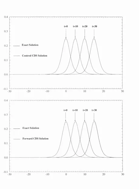
conservative and phase properties are studied for th e centred CDS. N um erical

experim ents in this chapter then show th a t favourable results are obtained by th e

proposed CDS, com pared w ith other m ethods for th e KdV equation.

In chapter four, huid-dynam ics theory is discussed regarding th e collapse of

an unsteady interacting boundary layer and th e developm ent of shortened length

and tim e scales, in th e near-wall dynamics of internal or external transitional-

tu rb u len t boundary layers or during dynam ic stall. The chapter is a join t sub­

m itte d paper w ith Prof. J.D .A . W alker, Dr. R.I. Bowles & Prof. F .T . Sm ith.

This is for large values of the characteristic Reynolds num ber. F in ite-tim e break­

up of th e unsteady interacting boundary layer occurs first. T he next stage th en

is described, where norm al pressure gradients come into operation along w ith a

continuing nonlinear critical-layer jum p. The theoretical study yields for certain

internal flows an extended KdV equation and for external or quasi-external flows

surface pressure. It is found th a t solution properties of these evolution equations

depend on th e signs of a coefficient jl m ultiplying th e Cauchy principal-value inte­

grals in th e equations. Therefore both th e theoretical account in this ch ap ter and

th e num erical study in the subsequent chapters are presented for zero, positive

and negative values of th e param eter /t for th e extended KdV and B enjam in-O no

equations, respectively.*

In fact, a higher-order scheme itself does not m ean higher accuracy. Sufficient

accuracy of com putation is essentially ensured by two factors: th e accuracy of

“resolution” of elem entary p arts of th e phenom enon under consideration and the

accuracy of th e algorithm itself. The first factor is associated w ith th e construc­

tion of difference meshes ensuring a sufficient num ber of points in th e subdom ains

of th e com putational dom ain which have th eir local characteristic size. One of

th e m ethods of constructing sub-difference meshes is by a coordinate transfor­

m atio n , which provides a unique characteristic scale in th e new variables, w ith a

subsequent uniform distribution of m esh points. Thus, w ith this kind of transfor­

m atio n , th e approxim ation error of the difference algorithm depends on th e order

of accuracy of th e scheme and on the higher-order derivatives of th e solution of the

differential equations w ith respect to th e new variables. Hence th e “resolution”

of m eshes is directly related to th e real accuracy of th e difference scheme, i.e.

an appro p riate transform ation of coordinates m ay result not only in an optim al

arrangem ent of mesh-points, b u t also in sm oothing of abruptly-varying functions.

For our problem s, we may expect solutions to develop singularities or some forms

of ab ru p t variation around th e origin (say) a t some tim es. Therefore in chap­

te r five, after an asym ptotic expansion is carried out to deal w ith th e boundary

conditions at infinity, a coordinate transform ation is form ulated to cluster th e

m esh points into th e range w ith th e most rapid variation of the solution. This

transform ation plays the role of stretching th e grid in one coordinate direction,

which tu rn s out to be very effective in the com putations presented in th e following

chapters six and seven.

Also in chapter five, first-, second- and third-order form ulae are derived to

handle th e Cauchy principle-value integrals, using Taylor expansions. T hen we

reach the point at which to form ulate th e whole algorithm for th e extended K dV

and B enjam in-O no equations w ith nonzero p aram eter ji. Here we adopt a dif­

ferent strategy from th a t applied by Prof. Frank Sm ith w ith Dr. J.M . Hoyle

rep o rted in Hoyle (1991) and th a t applied by David W alker and Ju n He (private

com m unications 1994 w ith W alker), which lag th e com putation of th e Cauchy

integrals at each tim e level. The iteration for the Cauchy integrals is done to

11

ensure th a t th e governing equation is satisfied closely. A lthough this tre a tm e n t

is som ewhat tim e-consum ing, the com putations carried out in chapters six and

seven seem to show th a t its good perform ance in capturing th e singularity and

resolving th e short waves in th e solutions is w orth th e effort.

In chapter six, first, th e com putation for zero /x, i.e. th e stan d ard K dV equa­

tio n along w ith unusual boundary conditions, is carried out in b o th th e physical

and th e transform ed planes. The theoretical study for this K dV equation at large

tim e is given in section 4.6 of chapter four. Second, th e com putation for positive

jl in th e transform ed plane clearly dem onstrates a fu rth er finite-tim e singularity.

T he theoretical local account for this phenom enon is also given in chapter four.

T he com putation for negative ji suggests, th ird , th e presence of a short-wave

instability. In chapter four, an analytical explanation is given, which leads to

a form ula for th e tem poral growth rate of any short-wave disturbance. T here­

fore th e final section of chapter six is devoted to com paring th e form ula, by th e

calculation of th e num erical growth rates.

The com putation for th e Benjam in-Ono equation and th e extended Benjam in-

Ono equation is done in chapter seven. The num erical results show a p a tte rn

sim ilar to th a t in th e KdV or extended KdV cases. Thus th e solution w ith zero

jl develops a beautiful traveling wave packet at larger tim e, and num erically it

seems this travel can be m aintained accurately for a very long tim e provided th a t

sufficiently sm all grid spacings and tim e steps are taken. Again, th e solution w ith

nonzero ji develops th e fu rth er finite-tim e singularity or short-wave instability,

depending on th e signs of ji and another p aram eter in th e equation.

Finally, fu rth er com m ents and suggestions for future study are given in chapter

C hapter 2

C om pact D ifference Schem es

2.1

In tr o d u c tio n

A higher-order m ethod coupled w ith easily solvable system s is clearly

desirable for th e num erical sim ulation of a fluid problem . High order of accuracy

is usually sought for th e spatial differential operator. Higher-order schemes can

be constructed by th e classical finite-difference approxim ations, which essentially

apply a linear com bination of functional values at some discretization points to

approxim ate derivatives of th e function. However, th e higher th e approxim ation

th e higher th e num ber of discretization points involved. In this way, a fourth-

order accurate m ethod generally involves five points and consequently leads to an

algebraic system w ith a pentadiagonal m atrix , and th e boundaries also require

special consideration, since fictitious points near b o th boundaries are created.

G enerally speaking, three-point hnite-difference discretization, which forms th e

basis for th e overwhelming m ajority of num erical solutions of th e equations of

fluid m echanics, is desired, since th e resulting algebraic m atrix system is of a

tridiagonal or block-tridiagonal form; therefore an efficient and well developed

two-pass algorithm (A hlberg et al., 1967) can be applied to invert th e m atrix

operator, and no fictitious point near th e boundaries is created. A nother way

to construct higher-order schemes which has th e above advantage is th e use of

“co m p act” m ethods. The basic idea of this m ethod is to introduce new variables

(generally th e derivatives of solution) instead of new discretization points, and

relationships among the variables and functions at three adjacent m esh points,

to form a closed coupled system together w ith th e differential equation as well

schemes in th e above sense, which is more general th a n K reiss’ original suggestion

(O rszag & Israeli, 1974) on “com pact differencing” (it is this suggestion th a t

sparked th e application and study of this class of higher-order schem es), say

H erm itian collocation , Fade approxim ation, and polynom ial spline, and K reiss’

com pact scheme can be generated from any of them ; see R ubin &: Khosla (1976).

Since K reiss’ suggestion, m any higher-order schemes have been generated using

th e above strategy and have been applied to various fluid problem s (H irsh 1975,

R ubin & Khosla 1976, Berger et al 1980 and A ubert & Deville 1983), especially

in recent years, and the application of higher order com pact difference schemes

to fluid problem s has become more usual practice; see Rohichi & Floryan (1995),

Adam s & Shariff (1996), W einan & Liu (1996), Fu & M a (1997), R avichandran

(1997), Yee (1997) and Jeon (1997).

Basically th ere are two different classes of com pact finite-difference schemes.

T he m ethods developed by Berger et al (1980), Cim ent & Leventhal (1975,1978b),

C im ent et al (1978a) and Leventhal (1982) can be regarded as one class derived

from a tre a tm e n t of th e whole differential equation, as distinct from th e oth er class

of com pact differencing m ethods which has been used by Hirsh (1975), and by

A ubert & Deville (1983), where derivatives are approxim ated individually to high

order. Two different forms of upwinding for these two classes of com pact m ethods

have also been presented, for the reason th a t standard num erical solutions often

contain nonphysical oscillations in convection dom inated problem s, such as in

fluid flow at m oderate to large Reynolds num bers, see Berger et aL Leventhal

(1982) and C hristie (1985). In Christie (1985), C hristie applied th e stan d ard

com pact finite-difference scheme used by Hirsh (1975) to th e m odel problem

u (æ) — K u (x) = 0, X e [0,1], (2.1a)

u (0) = 1, u ( l) = 0, (2.1b)

where K is a positive constant. He showed th a t there exists a negative root in th e

characteristic polynom ial of a five point form ula which is equivalent to th e corre­

sponding stan d ard com pact scheme. This means th a t th e solution w ith th e stan ­

dard com pact scheme contains oscillations. In addition, the continued presence of

oscillatory solutions for a sim ilar problem was also noted by C im ent et al (1978a).

To remove th e oscillatory behavior, Christie introduced a free p aram eter into th e

stan d ard com pact scheme to produce upwind com pact finite-difference schemes

which can significantly dam p out oscillations through an optim al choice of th e

free param eter. In section 2.2 below, C hristie’s upwinding m ethod is am ended

A nother way to upwind K reiss’ com pact difference scheme is by th e use of

T olstykh’s nonsym m etric com pact scheme (Tolstykh, 1986). In section 2.3, a gen­

eral form which combines K reiss’ com pact scheme w ith Tolstykh’s nonsym m etric

schemes is given for B urgers’ equation. This scheme perm its th e application of up-

winding. A nd also in this section C hristie’s upwinding com pact difference scheme

is am ended to deal w ith a m ore general situation of nonlinear problem s. C om par­

isons of results from K reiss’s com pact scheme, C hristie’s scheme and T olstykh’s

scheme are m ade through num erical experim ents for two m odel problems.

2.2

E x te n d in g U p w in d C o m p a ct F in ite-D ifF

ere-n ce S ch em es

Consider th e 1-dimensional m odel problem:

u \ x ) — K u { x ) — Cu{x) = 0, æ G [0,1], (2.2a)

u (0) = 1, u ( l) = 0. (2.2b) If (7 = 0, (2.2) becomes (2.1). The characteristic equation of (2.2a) is

- K r - C = 0, (2.3)

and when A = + 4(7 > 0, (2.3) has two different real roots:

So, in this case, th e theoretical solution of (2.2) is found to be

pT-a® _ pT-2- r i ( l - x )

^ 1 _ grg-n •

Divide th e u n it interval into N equal subintervals [(i — l)/t,%/t], i = 1,2, • • JV,

where th e grid spacing h = 1/iV. Then the application of th e stand ard com pact

finite-difference scheme to (2.2a) gives

g (^i+ i + + -Pi-i) = ^ ( (7^+1 — (A -i), (2.6a) — (•S'i+i + 105i + S i- \) = — (C/j+i — 2Ui + t/i- i) , (2.6b)

where Fi and Si are approxim ations to th e first and second derivatives respec­

tively. These equations hold for z = l , 2, ••• ,i\T — 1 and (2,6c) also holds at

i = 1 , N . Therefore additional boundary conditions are required.

Taylor series expansions show th a t

Fi = U : ~ + • ■ • , (2.7a)

% = + • • • . (2-7b)

and so (2.6) is a fourth-order accurate tri diagonal system for th e solution of (2.2). Now we introduce an upwind param eter 7 into (2.6a) to give an altern ativ e form ula,

i( F i+ i+ 4 F i+ F i_ i) = ^ [( l-7 )C 7 i+ i+ 2 7 Î7 i-(l+ 7 )7 7 i_ i]. (2.8) Taylor series expansions here give the tru ncation error as

Fi = U',~ ^ C 7 (= ) - ÿ t / " + . • • , (2.9)

and so th e choice 7 = 0{h^) is necessary to m aintain fourth-order accuracy. For convenience, we use th e shift operator Ej which is defined as

E^fn = fn+j, j integer,

to express (2.6a) and (2.6b) as

P^{E)Fi^, =

1

[P

2

{E)

-

'yP4{E)]Ui.^,

(2.10a)

P3{E)Si-4 = ^ P 4( E )U i- 4, (2.10b)

where

Pi{E) = E^ + i E + 1, (2.11a)

P2(E) = E^ - I = {E + I ) { E - I ) , (2.11b)

P3{E) = E^ + 10Ê + I, (2.11c)

Pi{E ) = E^ - 2 E + I = { E - I f . (2.11d)

Using (2.6c) to elim inate Si from (2.10b) gives

P 2 {E )F i.i = F i i E ) — — Pî{E)

T hen (2.12) and (2.10a) lead to

= ^ [(2 + l L ) P , { E ) - PP^(E) - LP,{E)] U i.u (2.13)

where L = K h j 2 and (3 = CÀ^/6. Finally, su b stitu tio n of (2.13) into (2.10a) gives a five point formula:

[2P^{E)P^{E)+^LP^[E)P^{E)-I3P^{E)P^{E)

-LP2{E)P^{E)]Ui.2 = ^, (2.14)

whose characteristic equation is

2P i( r ) P4(r) + ')LP^[t)P^(t) - pPr{T)P^{v)

- LP2(r)P^{v) = 0. (2.15)

The quartic polynom ial (2.15) has four roots, which co n stitute th e solution of

(2.14). A nd we also know th a t r i and 7*2 are th e roots of th e characteristic equation of (2.2) and th a t and constitute th e exact solution. Therefore

we choose 7 to m ake or be a root of (2.15). In this way, we o b tain two calculation form ulae concerning th e upwind param eter 7:

and th en a series expansion shows th a t

+ 0((rife)=), (2.17a)

+ 0((r2ft)=). (2.1Tb)

Thus 7i = 0{ h^) and 72 = 0{h^) for fixed K and C.

To close th e system (2.8), (2.6b) and (2.6c), we need two additional boundary

equations. Here a Fade type of approxim ation is used:

U i — U i+ i + / i [ a P i + ( l — o : ) P i + i ] + — [ ( a — - )5'i + ( o i — - )5'j+i] = 0,

(2.18a)

or

- P , { E ) U i + h [ - a P s { E ) + E ] F i + ~ [ a P s { E ) - \ p , { E ) ] S i = 0,

where

Ps{E) = E - I , Pe{E) = E - \ - I , P7(E ) = 2 E L (2.19)

T he form ula is of fifth order when o:=0.5 and fourth order otherwise.

In order to upw ind the boundary relations, firstly, using (2.6c) to elim inate

Si from (2.18) and solving (2.18) for a gives

_ [P5( g ) + ^ P7(E)]Ui + [ ~ h E + f P r ( E ) ] F j

“ ZpP^{E)Ui + \ - h P ^ { E ) + hLP^{E)]Fi ■ ^

Secondly, su bstituting Ui = and 7 = 71 into (2.13) gives Finally, su bstitu tio n of (2.21) and Ui = into (2.20) leads to

-/i^(7e"^^[c/i(ri/i) + 5] + [(6 -5 L )e " ^ ^ -(6 + 8 T )+ T e -" ^ ^ ](e ^ ^ ^ -l) — h^C{e^^^ — l)[ch{rih)-\-b] + 12(e’‘^^ — l)[ch{rih) — Ls h{rih ) — 1]

I I

ai

Similarly, we have

— [ch(r2 /i) + 5] + [(6 — 5T)e^^^ — (6+ 8T) + (e^^^ — 1)

0L2

—h^C{e^^^ — 1 ) [ch{r2h) + 5] + 12(e’"2^ — 1 ) [ch{r2h) — Lsh[r2h) — 1]

( Z.ZZD I

W hen C = 0, 7i and cli coincide w ith th e optim al 7 and a obtained by C hristie in (C hristie, 1985), and th en 72 = 0, «2 = i.e. th e stan d ard com pact scheme is retrieved.

We call th e two com pact schemes corresponding to (71, oti) and (72, «2) “upw ind schemes (I) and (II)” respectively. It will be seen later th a t th ey produce

different behaviors.

The system (2.8), (2.6b) and (2.6c) is tri diagonal, and if th e Ui are given, it is easily solved for th e Fi and Si. If the Ui are unknowns th en ordering th e

unknowns as C/^, Fi and Si for each i gives a block tri diagonal system w ith 3

X 3 blocks. Here our interest is in im plicit com pact schemes. We use (2.6c) to

elim inate th e Si in (2.6b) and then order th e unknowns as Ui and Fi for each i to give a 2x2 block tri diagonal system.

^ h/ 2 = D [ h j 2 y are two successive m axim um errors then th e ra te p is estim ated

from

(2.23)

T he com puted rates agree closely w ith th e theoretical order of th e m ethods.

In T a b le 2.5 -2 .7 , some num erical results are presented to show th e extent of th e oscillations in the standard compact scheme (2.6) applied to (2.2) for a variety of K and C values, and th e num erical solutions from C hristie’s upw ind

scheme and our upw ind schemes (I) and (II) are also shown in th e tables. Here

th e relative error is defined as {u[xi) — Ui}lu(xi), from which oscillatory behavior

can be observed. From these tables, it is observed th a t for large K and sm all C

b o th C hristie’s scheme and scheme (I) significantly dam p out th e oscillation, b u t

scheme (I) is th e more accurate, while for small K and large C C hristie’s scheme

does not work well while scheme (II) does. Again, for th e case of nonoscillation

in th e solution of the stan d ard com pact scheme, th e upw ind scheme (I) or (II)

can also achieve a higher accuracy.

N

Nonupwind Christie’s Scheme (I) Scheme (II)

Error Rate Error Rate Error Rate Error Rate

10 3.05D-2 1.12D-2 9.12D-3 3.07D-2

20 2.93D-3 3.38 1.20D-3 3.22 1.03D-3 3.15 2.95D-3 3.38

40 2.27D-4 3.69 9.67D-5 3.63 8.51D-5 3.59 2.29D-4 3.69

80 1.57D-5 3.85 6.84D-6 3.82 6.11D-6 3.80 1.58D-5 3.85

160 1.03D-6 3.93 4.54D-7 3.91 4.09D-7 3.90 1.04D-6 3.93

320 6.63D-8 3.96 2.93D-8 3.96 2.64D-8 3.95 6.65D-8 3.97

Table 2.1: Convergence Rates for Maximum Error in F: Problem (2.2) with ÜT = 10 and C = 10.

The extension of th e above upwind com pact m ethods to tim e-dependent prob­

lems is straightforw ard. The test problem here is

- K u ^ — C u = (x, t) G [0, l ] X [0, Oo),

n (0,t ) = 1, = 0, t > 0, u (x ,0) = 1, u ( l ,0) = 0, 0 < X < 1,

(2.24a)

(2.24b)

(2.24c)

where th e constants i/, K and C satisfy  = -f- 4i/(7 > 0. T he exact solution

of (2.24) can be found by th e m ethod of separation of variables (see A ppendix

u { x ,t)

f2X_^r2-ri{l-x) ^

Cn = Smru

I —x'ST^ • / \ _iiAôd±*!±â«iÉ.t

1-62" > Cnsin(n7ræ)'e 4^

,

n=l

a

where ri and V2 are defined as follows;

k + \ /a k - V X

n = ---- ;;---, ’’2 =

(2.25a)

(2.25b)

2u 2u (2.26)

Obviously, (2.24) has a steady solution, and when C is zero, (2.24) becomes th e

convection-diffusion problem th a t was dealt w ith by C hristie (1985).

For fixed x, (2.24a) is an ordinary differential equation and so th e application

of ^-m ethods for the ODE gives

A t = 6

+ ( ! - « )

dx^ dx

d‘^U^{x) ^ d U ^ x )

dx^ dx - CU^{x) (2.27)

where A t is th e tim e step, = n A t , and U^{x) is th e approxim ation to u{x,tn).

T he tru n catio n error is

(2.28)

Therefore this discretization in th e t-direction is of second-order accuracy ii 6 = ^

b u t first-order accuracy otherwise. (2.27) can be rew ritten as

_ ( C + C )u * { x ) = - c a " ( æ ) ,

dx^ dx

where C = ^ and

u'(x)

eu’^+\x)

(1

e)ir{x).

T he in itial condition on (2.29a) is

U^{x) = u (0, ®) = 1, and th e b oundary conditions are

î/*(o) = dî/"+'(o) + (1 - g)cr(o) = 1,

17*(1) = flC;"+i(l) + (1 - B)U"{\) = 0,

(2.29a)

(2.29b)

(2.29c)

(2.29d)

since Î7*(0) = u (0 ,ti) = 1 and C/*(l) = u ( l , t i ) = 0 for any integer i. Therefore, at

each tim e step, com pact finite-difference schemes can be applied to th e boundary

value problem for th e ordinary differential equation (2.29) and so th e algorithm

applied earlier to (2.2) can be used j after slight am endm ent of this problem . In form ulae (2.16) and (2.22), we use K = K j v and C = C /f/, while and T2 are calculated w ith (2.26). Num erical results for this problem are displayed

on T a b le 2.8-2.1 0, The num erical behavior for this tim e-dependent problem is found to be th e same as th a t for problem (2.2).

The convergence rates given in T a b le 2 .2 were also obtained from (2.23). Values of Æ = 10, C = 10 and v = 1 were chosen and th e solutions were

com pared at t = 0.4, æ = 0.9. The mesh was reduced according to A t = h^.

Close agreem ent w ith th e theoretical order p = 4 was also found for this tim e-

dependent problem.

N

Steps M

Nonupwind Christie’s Scheme (I) Scheme (II)

Error Rate Error Rate Error Rate Error Rate

20 160 1.28D-5 7.87D-7 1.35D-6 1.30D-5

40 640 7.43D-7 4.11 5.90D-8 3.74 9.23D-8 3.87 7.46D-7 4.11

80 2560 4.41D-8 4.07 3.69D-9 4.00 5.89D-9 3.97 4.43D-8 4.07

160 10240 2.72D-9 4.02 2.3D-10 4.00 3.7D-10 3.99 2.73D-9 4.02

Table 2.2: Convergence Rates for (2.24) : Æ = 10, C = 10, %/ = l , u ( x , t ) , t = 0.4, x 0.9, At = h = 1/N, At -- OAfM.

N At M u(x,t) : X = 0.9, t = 0.4 Rates

80 160 320 640 6.25E-3 1.5625E-3 3.90625E-4 9.765625E-5 64 256 1024 4096 0.63214510669621 0.63214488298773 0.63214486844268 0.63214486749075 3.94 3.93

Table 2.3: Christie’s results: Convergence Rates for (2.24) with K = 10, C = 0, u

1, At = h = 1/N, At — 0.4/M.

O ur results for zero C are sim ilar to C hristie’s, b u t different. In p articu lar our

results for th e convergence rates { K = 10, C = 0, u = 1, t = 0.4) converge to th e

exact solution (2.25a,b); see A ppendix A and T a b le s 2.3 & 2 .4 . C h ristie’s agree

N A t M u{x,t) : X = 0.9, t = 0.4 Rates 80

160 320 640

6.25E-3 1.5625E-3 3.90625E-4 9.765625E-5

64 256 1024 4096

0.63213969086475 0.63214928653246 0.63214928793975 0.63214928794838

12.7 7.35

Table 2.4: Our results: Convergence Rates for (2.24) with K = 10, C = 0, u = 1, A t = h?, h = 1/N, A t = 0.4/M . The exact value of u(0.9,0.4) is 0.63214928794767 •••, which is obtained from (2.25); see Appendix A.

rates were calculated from

P = _In

2In

Uh — Uh/2

Uh/2 — Uih/4j (2.30)

regardless of the known analytical solution (2.25). We also notice th a t th e con­

vergence rates m ay vary considerably at finite N before tending to th e large N

K ,C Exact Nonupwind Christie’s Scheme (I) Scheme (II)

h X u{x) Rel. Error Rel. Error Rel. Error Rel. Error

0.0 1.0000 O.OOD+00 O.OOD+00 O.OOD+00 O.OOD+00

0.1 0.9950 0.695D-04 0.167D-06 0.280D-07 0.696D-04

0.2 0.9901 -0.542D-04 -0.726D-07 0.515D-07 -0.542D-04

i f = 20 0.3 0.9851 0.211D-03 0.528D-06 0.759D-07 0.211D-03

0.4 0.9802 -0.368D-03 -0.709D-06 0.998D-07 -0.368D-03

C = 1 0.5 0.9753 0.903D-03 0.199D-05 0.125D-06 0.903D-03

0.6 0.9702 -0.186D-02 -0.434D-05 0.147D-06 -0.186D-02

h = 0.1 0.7 0.9634 0.434D-02 0.662D-05 0.175D-06 0.434D-02

0.8 0.9436 -0.836D-02 -0.321D-04 0.192D-06 -0.836D-02

0.9 0.8280 0.304D-01 0.377D-05 0.232D-06 0.304D-01

1.0 0.0000 O.OOD+00 O.OOD+00 O.OOD+00 O.OOD+00

Maximum 0.304D-01 0.321D-04 0.232D-06 0.304D-01

0.0 1.0000 O.OOD+00 O.OOD+00 O.OOD+00 O.OOD+00

0.1 0.9070 0.923D-02 -0.656D-03 -0.776D-03 0.937D-02

0.2 0.8226 -0.539D-02 -0.122D-02 -0.146D-02 -0.546D-02

K = 40 0.3 0.7461 0.206D-01 -0.183D-02 -0.217D-02 0.209D-01

0.4 0.6767 -0.261D-01 -0.236D-02 -0.286D-02 -0.264D-01

C = 40 0.5 0.6138 0.579D-01 -0.306D-02 -0.358D-02 0.587D-01

0.6 0.5567 -0.932D-01 -0.339D-02 -0.423D-02 -0.945D-01

h = 0.1 0.7 0.5049 0.18D+00 -0.455D-02 -0.504D-02 0.18D+00

0.8 0.4579 -0.31D+00 -0.395D-02 -0.550D-02 -0.32D+00

0.9 0.4091 0.56D+00 -0.109D-01 -0.677D-02 0.56D+00

1.0 0.0000 O.OOD+00 O.OOD+00 O.OOD+00 O.OOD+00

Maximum 0.56D+00 0.109D-01 0.677D-02 0.56D+00

0.0 1.0000 O.OOD+00 O.OOD+00 O.OOD+00 O.OOD+00

0.1 0.9070 0.362D-08 0.536D-05 -O.lOlD-05 0.231D-09

0.2 0.8226 -0.376D-07 0.104D-04 -0.196D-05 -0.443D-07

K = 40 0.3 0.7461 -0.434D-06 0.153D-04 -0.300D-05 -0.445D-06

0.4 0.6767 -0.214D-05 0.204D-04 -0.392D-05 -0.216D-05

C = 40 0.5 0.6138 -0.114D-04 0.252D-04 -0.489D-05 -0.115D-04

0.6 0.5567 -0.603D-04 0.292D-04 -0.583D-05 -0.606D-04

h = 0.05 0.7 0.5049 -0.319D-03 0.288D-04 -0.681D-05 -0.320D-03

0.8 0.4579 -0.168D-02 0.245D-05 -0.775D-05 -0.168D-02

0.9 0.4091 -0.835D-02 -0.249D-03 -0.864D-05 -0.839D-02

1.0 0.0000 O.OOD+00 O.OOD+00 O.OOD+00 O.OOD+00

Maximum 0.299D-01 0.249D-03 0.942D-05 0.300D-01

K , C Exact Nonupwind Christie’s Scheme (I) Scheme (II)

h X u{x) Rel. Error Rel. Error Rel. Error Rel. Error

0.0 1.0000 O.OOD+00 O.OOD+00 O.OOD+00 O.OOD+00

0.1 0.9995 -0.67D+00 -0.734D-07 -0.726D-07 -0.21D+01

0.2 0.9990 0.891D-01 -0.151D-06 -0.153D-06 0.34D+00

K = 1Q2 0.3 0.9985 -0.83D+00 -0.256D-06 -0.246D-06 -0.26D+01

0.4 0.9980 0.29D+00 -0.251D-06 -0.289D-06 0.98D+00

C = 0.5 0.5 0.9975 -O.llD+01 -0.553D-06 -0.404D-06 -0.34D+01

0.6 0.9970 0.59D+00 0.109D-06 -0.469D-06 0.19D+01

h = Q.l 0.7 0.9965 -0.14D+01 -0.279D-05 -0.547D-06 -0.45D+01

0.8 0.9960 O.lOD+01 0.810D-05 -0.628D-06 0.33D+01

0.9 0.9955 -0.19D+01 -0.725D-04 -0.716D-06 -0.60D+01

1.0 0.0000 O.OOD+00 O.OOD+00 O.OOD+00 O.OOD+00

Maximum 0.19D+01 0.725D-04 0.716D-06 0.60D+01

0.0 1.00000 O.OOD+00 O.OOD+00 O.OOD+00 O.OOD+00

0.1 0.40450 0.158D-02 0.161D-02 -0.678D-03 0.112D-07

0.2 0.16370 0.289D-02 0.290D-02 -0.112D-02 -0.275D-07

K = 2 0.3 0.06621 0.437D-02 0.439D-02 -0.171D-02 -0.134D-07

0.4 0.02678 0.573D-02 0.575D-02 -0.221D-02 -0.413D-07

C = 10^ 0.5 0.01083 0.717D-02 0.718D-02 -0.277D-02 -0.242D-06

0.6 0.00438 0.855D-02 0.857D-02 -0.329D-02 -0.115D-05

h = 0.1 0.7 0.00177 0.994D-02 0.996D-02 -0.385D-02 -0.994D-05

0.8 0.00071 0.112D-01 0.112D-01 -0.437D-02 -0.341D-04

0.9 0.00025 0.123D-01 0.123D-01 -0.622D-02 -0.438D-03

1.0 0.00000 O.OOD+00 O.OOD+00 O.OOD+00 O.OOD+00

Maximum 0.123D-01 0.123D-01 0.622D-02 0.438D-03

0.0 1.00000 O.OOD+00 O.OOD+00 O.OOD+00 O.OOD+00

0.1 0.09861 0.23D+00 0.25D+00 -0.60D+00 0.146D-07

0.2 0.00972 0.23D+00 0.20D+00 -O.llD+01 0.322D-07

K = 20 0.3 0.96D-3 0.65D+00 0.71D+00 -0.24D+01 0.196D-07

0.4 0.95D-4 0.931D-01 -0.214D-01 -0.32D+01 0.342D-07

C = 10^ 0.5 0.93D-5 0.15D+01 0.18D+01 -0.62D+01 -0.307D-08

0.6 0.92D-6 -0.13D+01 -0.18D+01 -0.76D+01 0.686D-06

h = 0.1 0.7 0.91D-7 0.48D+01 0.60D+01 -0.15D+02 -0.217D-04

0.8 0.89D-8 -0.83D+01 -0.12D+02 -0.16D+02 0.713D-03

0.9 0.88D-9 0.32D+02 0.58D+02 -0.58D+02 -0.252D-01

1.0 0.00000 O.OOD+00 O.OOD+00 O.OOD+00 O.OOD+00

Maximum 0.32D+02 0.58D+02 0.58D+02 0.252D-01

K ,C Exact Nonupwind Christie’s Scheme (I) Scheme (II)

h X u{x) Rel. Error Rel. Error Rel. Error Rel. Error

0.0 1.00000 O.OOD+00 O.OOD+00 O.OOD+00 O.OOD+00

0.1 0.09861 0.210D-04 0.229D-04 -0.251D-04 0.146D-07

0.2 0.00972 0.418D-04 0.455D-04 -0.502D-04 0.322D-07

K = 20 0.3 0.00096 0.626D-04 0.680D-04 -0.754D-04 0.196D-07

0.4 0.95D-4 0.834D-04 0.906D-04 -O.lOlD-03 0.336D-07

C = 1 0^ 0.5 0.93D-5 0.104D-03 0.113D-03 -0.126D-03 0.170D-07

0.6 0.92D-6 0.125D-03 0.136D-03 -0.151D-03 0.255D-07

h = 0 . 0 1 0.7 0.91D-7 0.146D-03 0.158D-03 -0.176D-03 0.264D-07

0.8 0.89D-8 0.167D-03 0.181D-03 -0.201D-03 0.213D-07

0.9 0.88D-9 0.190D-03 0.200D-03 -0.230D-03 -O.llOD-06

1.0 0.00000 O.OOD+00 O.OOD+00 O.OOD+00 O.OOD+00

Maximum 0.195D-03 0.212D-03 0.246D-03 0.510D-05

Table 2.7: Numerical Solution of (2.2) Using Compact Difference schemes. 0 = h

K ,C ,u Exact Nonupwind Christie’s Scheme (I) Scheme (II)

h, At, t X u(cc,<) Rel. Error Rel. Error Rel. Error Rel. Error

0.0 1.0010 O.OOD+00 O.OOD+00 O.OOD+00 O.OOD+00

K = 102 0.1 1.0010 -0.13D+02 -0.490D-06 -0.489D-06 -0.13D+02

0.2 1.0020 0.400D-01 -0.986D-06 -0.986D-06 0.525D-01

C = - l 0.3 1.0030 -0.13D+02 -0.146D-05 -0.146D-05 -0.13D+02

0.4 1.0040 0.32D+00 -0.198D-05 -0.198D-05 0.33D+00

V —0.1 0.5 1.0050 -0.14D+02 -0.243D-05 -0.243D-05 -0.14D+02

0.6 1.0060 0.60D+00 -0.298D-05 -0.296D-05 0.61D+00

h = 0.1 0.7 1.0070 -0.14D+02 -0.320D-05 -0.341D-05 -0.14D+02

0.8 1.0080 0.89D+00 -0.577D-05 -0.393D-05 0.91D+00

At = 0.01 0.9 1.0090 -0.14D+02 0.161D-03 -0.441D-05 -0.14D+02

1.0 0.0000 O.OOD+00 O.OOD+00 O.OOD+00 O.OOD+00

t = 1 Maximum 0.14D+02 0.161D-03 0.441D-05 0.14D+02

0.0 1.0000 O.OOD+00 O.OOD+00 O.OOD+00 O.OOD+00

K — 20 0.1 0.9950 0.695D-04 0.167D-06 0.281D-07 0.696D-04

0.2 0.9901 -0.541D-04 -0.726D-07 0.515D-07 -0.542D-04

C = 1 0.3 0.9852 0.211D-03 0.526D-06 0.759D-07 0.211D-03

0.4 0.9802 -0.368D-03 -0.709D-06 0.998D-07 -0.368D-03

u = 1 0.5 0.9753 0.903D-03 0.199D-05 0.125D-06 0.903D-03

0.6 0.9702 -0.186D-02 -0.435D-05 0.147D-06 -0.186D-02

h —0.1 0.7 0.9634 0.434D-02 0.662D-05 0.175D-06 0.434D-02

0.8 0.9436 -0.836D-02 -0.321D-04 0.192D-06 -0.836D-02

At = 0.01 0.9 0.8280 0.304D-01 0.377D-05 0.232D-06 0.304D-01

1.0 0.0000 O.OOD+00 O.OOD+00 O.OOD+00 O.OOD+00

t = 1 Maximum 0.304D-01 0.321D-04 0.232D-06 0.304D-01

Exact Nonupwind Christie’s Scheme (I) Scheme (II) /i, Af, t X u { x ^ t ) Rel. Error Rel. Error Rel. Error Rel. Error

0.0 1.0000 O.OOD+00 O.OOD+00 O.OOD+00 O.OOD+00

K = 1Q2 0.1 0.9995 -0.67D+00 -0.789D-07 -0.781D-07 -0.21D+01

0.2 0.9990 0.891D-01 -0.150D-06 -0.153D-06 0.34D+00

C = 0.5 0.3 0.9985 -0.83D+00 -0.238D-06 -0.228D-06 -0.26D+01

0.4 0.9980 0.29D+00 -0.264D-06 -0.303D-06 0.98D+00

u — 1 0.5 0.9975 -O.llD+01 -0.527D-06 -0.378D-06 -0.34D+01

0.6 0.9970 0.59D+00 0.126D-06 -0.452D-06 0.19D+01

h = 0.1 0.7 0.9965 -0.14D+01 -0.278D-05 -0.530D-06 -0.45D+01

0.8 0.9960 O.lOD+01 0.813D-05 -0.598D-06 0.33D+01

Af = 0.01 0.9 0.9955 -0.19D+01 -0.725D-04 -0.694D-06 -0.60D+01

1.0 0.0000 O.OOD+00 O.OOD+00 O.OOD+00 O.OOD+00

t = 1 Maximum 0.19D+01 0.725D-04 0.694D-06 0.60D+01

0.0 1.0000 O.OOD+00 O.OOD+00 O.OOD+00 O.OOD+00

K = 10^ 0.1 0.9995 -O.llD+02 -0.124D-06 -0.124D-06 -0.12D+02

0.2 0.9990 0.500D-01 -0.242D-06 -0.242D-06 0.483D-02

C = 0.5 0.3 0.9985 -0.12D+02 -0.372D-06 -0.372D-06 -0.12D+02

0.4 0.9980 0.32D+00 -0.481D-06 -0.482D-06 0.28D+00

u =0.1 0.5 0.9975 -0.12D+02 -0.622D-06 -0.621D-06 -0.12D+02

0.6 0.9970 0.59D+00 -0.712D-06 -0.724D-06 0.55D+00

h = 0.1 0.7 0.9965 -0.12D+02 -0.970D-06 -0.864D-06 -0.12D+02

0.8 0.9960 0.88D+00 -0.367D-07 -0.973D-06 0.85D+00

Af = 0.01 0.9 0.9955 -0.13D+02 -0.836D-04 -O.llOD-05 -0.13D+02

1.0 0.0000 O.OOD+00 O.OOD+00 O.OOD+00 O.OOD+00

t = \ Maximum 0.13D+02 0.836D-04 O.llOD-05 0.13D+02

0.0 1.0000 O.OOD+00 O.OOD+00 O.OOD+00 O.OOD+00 i f = 40 0.1 0.9070 -0.666D-08 0.535D-05 -0.102D-05 -O.lOlD-07

0.2 0.8226 -0.660D-07 0.104D-04 -0.199D-05 -0.726D-07

C = 40 0.3 0.7461 -0.394D-06 0.154D-04 -0.296D-05 -0.405D-06

0.4 0.6767 -0.214D-05 0.204D-04 -0.392D-05 -0.216D-05

u = 1 0.5 0.6138 -0.114D-04 0.252D-04 -0.489D-05 -0.115D-04

0.6 0.5567 -0.603D-04 0.292D-04 -0.585D-05 -0.606D-04

/i = 0.05 0.7 0.5049 -0.319D-03 0.288D-04 -0.682D-05 -0.320D-03

0.8 0.4579 -0.168D-02 0.243D-05 -0.777D-05 -0.168D-02

Af = 0.01 0.9 0.4091 -0.835D-02 -0.249D-03 -0.866D-05 -0.839D-02

1.0 0.0000 O.OOD+00 O.OOD+00 O.OOD+00 O.OOD+00

t = 1 Maximum 0.299D-01 0.249D-03 0.942D-05 0.300D-01

\-Exact Nonupwind Christie’s Scheme (I) Scheme (II)

h , At, t X u(x,t) Rel. Error Rel. Error Rel. Error Rel. Error

0.0 1.0000 O.OOD+00 O.OOD+00 O.OOD+00 O.OOD+00

K = 20 0.1 0.0986 0.210D-04 0.229D-04 -0.251D-04 -0.211D-14

0.2 0.0097 0.418D-04 0.454D-04 -0.503D-04 -0.250D-14

C = 10% 0.3 0.0010 0.626D-04 0.680D-04 -0.754D-04 -0.362D-14

0.4 0.9D-4 0.834D-04 0.906D-04 -O.lOlD-03 0.158D-14

Ï/ = 1 0.5 0.9D-5 0.104D-03 0.113D-03 -0.126D-03 0.654D-14

0.6 0.9D-6 0.125D-03 0.136D-03 -0.151D-03 0.115D-13

= 0.01 0.7 0.9D-7 0.146D-03 0.158D-03 -0.176D-03 -0.567D-12

0.8 0.9D-8 0.167D-03 0.181D-03 -0.201D-03 -0.292D-09

At = 10"3 0.9 0.9D-9 0.187D-03 0.203D-03 -0.226D-03 -0.109D-06

1.0 0.0000 O.OOD+00 O.OOD+00 O.OOD+00 O.OOD+00

t = 1 Maximum 0.195D-03 0.212D-03 0.246D-03 0.507D-05

0.0 1.0000 O.OOD+00 O.OOD+00 O.OOD+00 O.OOD+OO

K = 1Q2 0.1 1.0010 -0.69D+00 -0.311D-06 -0.313D-06 -0.69D+00

0.2 1.0020 0.898D-01 -0.616D-06 -0.611D-06 0.899D-01

C = —1 0.3 1.0030 -0.85D+00 -0.892D-06 -0.912D-06 -0.85D+00

0.4 1.0040 0.29D+00 -0.129D-05 -0.121D-05 0.29D+00

V = 1 0.5 1.0050 -O.llD+01 -0.121D-05 -0.151D-05 -O.llD+01

0.6 1.0060 0.59D+00 -0.298D-05 -0.181D-05 0.59D+00

h = 0.1 0.7 1.0070 -0.15D+01 0.240D-05 -0.211D-05 -0.15D+01

0.8 1.0080 O.lOD+01 -0.199D-04 -0.240D-05 O.lOD+01

At = 0.01 0.9 1.0090 -0.20D+01 0.141D-03 -0.277D-05 -0.20D+01

1.0 0.0000 O.OOD+00 O.OOD+00 O.OOD+00 O.OOD+OO

t = 1 Maximum 0.20D+01 0.141D-03 0.277D-05 0.20D+01

2 .3

C o m p a ct D ifferen ce S ch em es for th e B u r g ­

e r s ’ e q u a tio n

In this section, we tu rn to the application of CDS to a nonlinear equation,

B urgers’ equation

- uiia: = Uf, { x ,t) E [fl, 6] X [0, + oo). (2.31) Divide th e interval [a, b]into N equal subintervals [xk, Xk+i] (A; = 0,1, - - ,iV — 1),

where = xq kh [k = 1,2, ••• ,iV — 1), and grid spacing

h = [h — a ) j N. In the tim e direction, th e tim e step is At and = nAt . T he tim e discretization using ^-m ethod leads to

i^Uxx uUx — 0 /\f. (2.32)

a t th e t = tn~\-OAt level. Therefore th e application of th e stan d ard CDS to (2.32)

yields a set of nonlinear equations

g(-fi+i + + Fi^i) = — (f/i+i — U i-i), (2.33a)

^ ('5 'i+ i + lO^i + S i- i ) = — {Ui+i — 2Ui + U i-i), (2.33b)

uS. - UiFi = (2.33c)

where U{, F{ and Si are the approxim ations of u{xi,t)jUx[xi,t) and Uxx{xi,t) at t = tn-{- 9A t , respectively.

Now we reconstruct (2.33a), i.e. the relationship between th e function and its

first derivative. F irst, define

C[u{x)] h] = a iu '{ x — h) a2u'{x) + clzu'(x + h)

- ^ [ - ( 1 + '^)u{x - h)-\- 2'yu{x) + (1 - 7)u(æ + h)]. (2.34) T hen Taylor expansion shows th a t

C[u{x)', h] = c iu ’[x) + C2hu"{x) + c^h?u^^\x)

where

Cl = OL\ 0L2 OL:^ — 1, (2.36a)

C2 = — a , + (2.36b)

C3 = - ( a i + 0:3) — - j (2.36c)

C4 = - (0:3 - 0!i) + (2.36d)

C5 = — («1 + 0:3) - (2.36e)

Letting ci = C2 = C3 = 0, we have

2 — 3^7 2 2 -|- 3'y . .

«3 = ^2 ' ^2 = - , o:, = , (2.37a)

and

=

m-Finally, th e third-order form ula associated w ith (2.34) is obtained,

^ [ ( 2 - 3 7 ) ^ ;- i+ 8 F i + ( 2 + 3 7 ) i^ i+ i] = ^ [ - { l + j ) U i . , + 2'yUi + { l-y )U i+ i] . (2.38)

In fact, when 7 = ± 1 , (2.38) becomes Tolstykh’s third-order nonsym m etric (non­ centred) com pact difference scheme, the application of which is involved in a

forward scheme ( 7 — —1) and a backward scheme ( 7 = 1). W hen 7 = 0, (2.38)

recovers th e fourth-order sym m etric ( centred )scheme (2.33a).

Now we rew rite (2.33) in a general form

1 1 1

^2+j^t+j — ^ ^ 2 ^2+j^i+ji (2.39a)

j = - i j = - i

Y^('S'i+i + lOS'i -f S i- i ) = — {Ui+i — 2Ui U i-i), (2.39b)

uSi - UiFi

=

(2.39c)

Here th e coeGicients in (2.39a) are related to i so th a t upw inding can be applied.

In detail, (2.39) could be any of th e following six schemes:

1. T olstykh’s third-order upwinding CDS:

7i = -s ig n { U l'), (2.40a)

= = = (2.40b)

This upwinding scheme is slightly different from Tolstykh’s original one

(Tolstykh, 1986), where a third-order form ula for U and S was adopted

instead of th e fourth-order form ula (2.39b),

2. The third-order forward CDS:

7i = - I j

, _ 5 , _ 2 , _ 1

12 ’ 3 ’ 12’

/

{

=

,

=

-

, /

* =

.

(2.41a)

(2.41b)

(2.41c)

3. The third-order backward CDS:

- 12’ 3 ’ " 12 ’

01 = - 1 , 02 = 1, 03 =

0-(2.42a)

(2.42b)

(2.42c)

4. The fourth-order centered CDS:

7i = 0,

.. 1

6’ i

-

01 = 02 = ^ ^ 0 3 = n '

i.e. th e stan dard CDS (2.33).

5. C h ristie’s upwinding CDS:

7i = 7 = coth(Jv) — — Jj

ch{2L) 4- 2

, _ 1 i _ 2 ■ _ 1 «1 g, «2 g, ^3 g,

1 -I- 'Y

=

-

=

,

=

ch(2L) + 5

1 - 7

(2.43a) (2.43b) (2.43c) (2.44a) (2.44b) (2.44c) (2.44d)

This is C hristie’s original version for B urgers’ equation. A pparently, th e

6. T he extended C hristie’s upwinding CDS: U^h

2 u ’ U^h

Li = (2.45a)

2

7i -= coth(i/i) - — ch{2Li^ T 2 ch{2Li) + 5

1

(2.45b)

<^2 — g ) ^3 ~ g ’ (2.45c)

= = = (2.45d)

In th e forthcom ing num erical experim ents, we will exam ine th e num erical

behavior of th e above schemes. Before th a t, th e basis of th e algorithm is described

as follows.

F irst, elim inating the 5^’s in (2.39b) using (2.39c) gives

R iU i-i + R2U i-\F i-i + R^Ui + 10722 Cft-Fj- + R\UiJf.\

+ 7 2 2 ( 7 , - R { U t i + lOUr + C^r+i) = 0, (2.46a)

where

/,2 /^2

72 = - -, 72i = 72—12, R2 — — , R3 = 1072+24. (2.46b)

1/{/ 1/

T hen th e system (2.39a) and (2.46a) is closed by th e boundary conditions

Uq — Ui + h[oiFo + (1 — q:)7^i] + h^[dQSo + di*?!] = 0, (2.47 a)

(7iv+/i[Q:FV_i+(l—o:)FV]+/i^[do<S’//_i+di»S'jv^] = 0, (2.47b)

or

?o(7o + QiUi + hpoFo + h [ l — ol-\ U\^F\

— 72(do(7j^ + diU^') = 0, (2.48a)

qoÜ N -i + 9i?7jv + h ( a H— ■ ^ U n - i ) F n - i + hp^Fj^

— R {d o U ^ _ i + d iU ^ ) = 0, (2.48b)

after elim inating 5"o, 5*1, S n - i , S n in (2.47) using (2.39c). Here

^0 = -^{oL — - ) , di = - ( a — - ) , (2.49a)

Ço — 1 T do72, q\ = —1 + di72, (2.49b)

Finally, elim inating Fq and in (2.39a) and (2.46a) yields a simplified nonlinear

system ,

— ■^(/5i + Di)Uo — — (/9g + D2)Ui + (cKg — Ds — D4Ui)Fi

— + 0:3 F2 + R { DzUq + DqUi ) = 0, (2.50a)

(^Ri — D7^Uq-{-[R3 — Ds)Ui-{- R2[—Dq-\-(^10 — Dio)Ui]Fi-\- R1U2

4 -7 Z 2 [/2 f2 -.R [(l-D n )(7 ^ + (1 0 -D i2 )[/r + C/r] = 0, (2.50b)

— ^U i-i-\-a \F i^ i — ^U i-\-o t2Fi — ^U n.i-\-a'2Fn.i = 0, (2.50c)

R iU i-i + R2U i-\Fi^i + RsUi + 10R2UiFi + R^Ui^i

+^2^7î+i-Fî+i — R{U^_^ + IOC/” + C/J]|_i), (2.50d)

2 = 2,3, • • • ^ N — 2,

Un-2-\-OLi ^Fn-2~ t { ^ 2 ^ + -^13)C/i\^-l+(q:^ ^ — D1 4 — Di5UN-i)F]sr-l

h h'

^ " b ^ i6)C/f\r4-^ ( ^ i7C/j}_2 + D igU ^) = 0, (2.50e) R l UN-2 + -ff2 C/N-2 Fn-2 + (R3 ~ Dig)UAT-l + R2 -^20 + (10 — D2 1 )UN-1 ] Fj^-i+ (i?i

-i^ 2 2 )c /N -i2 [c /jj_ 2 + (io -i)2 3 )c/;^ _ i+ (i-2 ?2 4 )c /;j]= o , (2.50f)

or

D {V ) = 0, (2.51)

where V = {U i,F i, C/2, F2, " • , C/at-i, FV _i)^, and

(2.52a)

Po Po

^ U o , Dg = (2.52c)

fipo Po

■- ^ U o , D i2 = ^ U o , (2.52d)

hpo hpo

a - a (2.52c)

Po

0=1 Adi

D:

ypo D,

D , = ^ U o , hpo

Adi

Dt

^10

—

C/q,

vpo N-l

F

D , 3 = " '

Pn N-l D Pn D 11 14 17

Pn J^Pn

D^s = (2.52f)

n _ -^290..

-^19 — T---hpN

-^22 — T Un^ hpN

T he Jacobian of (2.51) is

A l C2

B i A2 C3

a

D2 0 — — f/jv,

Pn

_

f/23 — T ^ N , hpN

D2 1 = — Un,

VpN _ R2di f / 2 4 — "7 Un

-hpN

(2,52g)

(2.52h)

J {V ) = B i - i Ai C,_i+l (2.53a)

A i =

Ai =

An-1 =

Bi =

C i =

B n - 3 A n - 2 C n- 1

B n - 2 A n - 1

~ h W2~^R^2) — B4Fi a \ — D3 — D4U1

R

— Dq-\-R2{10 — Dio)Fi R2\—

Dg-\-(^10 — Dio)Ui]

h

f?3 + 10ff2f^t lOff] (fit

, i = 2 , ‘ - , N - 2 ,

(2.53b)

(2.53c)

^ —Di sFn- 1 0L2 ^ — D\/i — Di^Un-1

R3 ~ Dig + J?2( 10 — D2i)Fn-1 R2 [~f^20 + ( 10 ~ f^21 )îfiV-l]

/3Î+' _i+l_a h

Rl

T

R2F{ R2Ui

F,

CLi - 1

h

'"3

R l + R2F{ R2Üi

) ^ — Ij 2, • • • , iV — 2,

, i = 2,3, • • • ,iV - 1.

Therefore Newton iteration for (2.51) is of th e form

yk+ i ^ y k _

or

j ( y O ) ( y * = + i _ y & ) = - D { V ^ ) .

(2.53d)

(2.53e)

(2.53f)

(2.54)

(2.55)

A fter finishing th e Newton iteratio n at t = + 9A t level, th e values of U and F

ai t = tn+i are calculated by

= [ U i - ( l - $ ) u n / S ,

l ,

, - - -

1

=

- (1 -

,i = 1,2,• • • , JV- 1 .

(2.56a)

T he first test problem is th e so-called “Moving Wave Front Problem ” , i.e. th e

solution of (2,31) satisfying Dirichlet boundary conditions and in itial conditions

consistent w ith th e analytical solution defined by

u { x , t ) = 0.1v4 T 0 .5 5 T C A + 5 + C

where

A — exp

B = exp

C = exp

-0.05(a: - 0.5 + 4.95t)

-0 .2 5 (3 - 0.5 + 0.75t)

(2.57)

(2.58a)

(2.58b)

(2.58c)

This problem was studied in Leventhal (1982), Sincovec (1977) and A l-R abeh

(1993). T he exact solution represents a moving wave front. T he steepness of th e

drop at th e front depends on v. The sm aller i> is th e steeper th e drop is, see

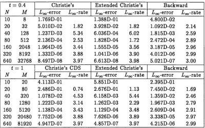
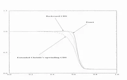
F ig u r e 2.1. Convergence results for v = 0.1 and 0.01 are given in T a b le 2.11

& 2 .1 2 , respectively, where Loo is defined as - 0.5(3 - 0.375)

Loo — m ax

u (2.59)

T a b le 2.1 1 shows th a t for a relatively m ild drop, u = 0.1, th e theoretical or­

ders of accuracy are confirmed. Here Tolstykh’s third-order upw inding CDS is

equavelent to th e backward CDS, since u is positive in th e whole range. For a

steep drop, however, u = 0.01, T a b le 2.1 2 shows th a t for this singular p e rtu r­

b atio n problem m ore mesh points are needed to m ain tain accuracy. G enerally

speaking, th e convergence property of C hristie’s upw inding CDS and th a t of the

extended C h ristie’s upw inding CDS is sim ilar, bu t they are quite different from

Tolstykh’s upw inding CDS, and th e la tte r has a b e tte r perform ance for relatively

large h [see T a b le 2.1 2 and F ig u r e s 2 .1 -2 .1 1], due to th e m onotonicity of th e

nonsym m etric scheme (see Tolstykh 1986). F ig u r e s 2 .1 -2 .1 1 show th e results

from th e centered, C hristie’s upwinding, th e extended C h ristie’s upw inding and

th e backw ard CDS for u = 0.003,0.001. The solutions by th e centered CDS

contain oscillations, and th e oscillations could persist for a certain range of de­

creasing grid spacings, depending on th e values of u. B oth C hristie’s upwinding

and th e backw ard CDS can dam p the oscillations, b u t th e backw ard CDS shows

a b e tte r perform ance. There is not m uch difference in results betw een C h ristie’s