The Effect of Openness on Economic Growth
for BRIC-T Countries: Panel Data Analysis
1Mehmet MERCAN
*, Ismet GOCER
**,Sahin BULUT
***, Metin DAM
∗∗∗∗Abstract
In this study, the effect of trade openness on economic growth was searched for the most rapidly developing countries (emerging markets; Brazil, Russia, India, China and Turkey, BRIC-T) via panel data analysis by using the annual data of the period from 1989 to 2010. As trade openness variable, the rate of external trade (Export+ Import) to GDP was used. According to empirical evidence derived from the study made with panel data analysis it was found that the effect of openness on economic growth was positive, and statistically significant in line with theoretical expectations.
Keywords: Trade Openness, Economic Growth, BRIC Countries, Turkey.
JEL Code Classification: E41, F43, G53
1 This study is the revised and altered version of the text presented at the conferences, 3rd International
Symposium on Sustainable Development(ISSD 2012), held in Sarajevo on May 31- June 1, 2010.
*
Asst. Prof. Dr., Hakkari University, Turkey. E-mail: mercan48@gmail.com, mehmetmercan@hakkari.edu.tr
**
Asst. Prof. Dr., Adnan Menderes University. Turkey. E-mail: ismetgocer@gmail.com
***
1. Introduction
In our globalized world whether there is a relationship between trade openness (openness hereafter) and economic growth and openness is useful for the economy of the countries or not is still a matter in argument. On one hand by trying to decrease the quotas and tariffs through GATT (General Agreement on Tariffs and Trade), UNCTAD (United Nations Conference on Trade and Development) which was established to liberalize the trade between countries and WTO (World Trade Organization) which was established instead of GATT in 1995, increasing the openness of the countries to the world trade is aimed, on the other hand countries impose restrictions in the world trade by increasing the invisible barrier both to protect the domestic industries and to get income.
With non-functioning of the national development thesis through the late 1970s and the collapse of the Eastern Block at the end of 1980s it was again started to argue that openness was necessary for the national economies. In this context some economists expressed that having a certain development level was a precondition for openness policies in order to support the growth while operating the growth models based on openness and export. (Han and Kaya, 2006: 245; Sun and Parikh, 2001: 187-188). There are classical economists on the basis of the view that capital movement liberalization and openness will increase the economic growth and welfare after 1980s. According to Classical and Neoclassical economists, foreign trade makes important contributions to the development and the foreign trade is not only an effective productivity instrument but also it is the engine of the growth. Since the sources are limited in developing countries, the production on the scale of a high and sustainable growth cannot be performed and new sources can be needed for production. With the openness, domestic markets will encounter with the competition, the domestic industries which cannot compete with international prices will transfer their production factor to the other productive factors and the welfare increase will happen as a result of more effective allocation of the sources. So, for this type of economies it will be useful to make production under free trade. The precondition of providing growth under free trade is to apply a foreign trade policy which the national economies may combine with the international structure and to direct the allocation of the sources for production to the sectors determined by the international demand. The natural aim of this type of economy is the industrialization and the availability of the growth and it is suggested that the required dynamism for this will be realized by a structuring coming from external demand rather than domestic demand (Celebi, 1991: 33).
different, but it would be useful among the countries that their development levels are the same. For instance, in England where the Industrial Revolution began first and in many of the other countries that were trying to reach England’s development level he expressed that free trade is on behalf of England and less developed countries were negatively affected for foreign trade relatively (Chang, 2004: 20).
Openness was modeled with the New Growth Theories suggested in 1980s and it was started to be tested empirically. Internal growth theories suppose that openness will stimulate the new technologies input (Harrison, 1996). No matter how the economy is open, technology input increases, technology usage becomes wide and a more rapid growth realizes as compared to a less open economy (Wu, 2004, s. 1). Internal growth models mentioning the importance of technological diffusion as the source of growth in long period generally suggest the thesis that the countries that are open to the foreign trade will reach higher steady growth rates (Grossman ve Helpman, 1990: 796). So Romer (1986) and Lucas (1988) expressed that the size of the openness in a country was proportional with the ability of adaptation to the new and imported technologies and the ability of the arrangement in production.
Shortly called as BRIC firstly in the early 2000s Brazil, Russia, India and China that have common characters like wide area, big population and rapid economic growth are accepted as the fastest growing “emerging market” in world economy (O’Neill, 2001:1-16). Total area of these countries contains more than 25% of the world area and total population of them contains more than 40% of the world population. It is argued that BRIC group would take G7 group’s place and get the leadership of the world economy when the economic indicators are considered (Frank and Frank, 2010:46-54). Goldman Sachs who has studies about BRIC countries estimates that in 2050 China will be the greatest economy in the world, India will be the third, Brazil will be the fourth and Russia will be the sixth biggest economy. Based on these indicators, in our study the effect of openness on economic growth will be searched for BRIC countries and Turkey that is the most developing country after China and has a developing economy.
2. Trade Openness
with the foreign trade volume increase. In Figure 1 trade openness rates of BRIC-T countries are presented.
Figure 1: BRIC-T Countries Trade Openness Rates
Source: It was formed by the authors using the World Bank data.
As can be followed from Figure 1, in all BRIC-T countries called as emerging markets since 1990s we have been observing a steady openness rates and the share of foreign trade increases. It has been seen that openness rate is about 0.5 in recent years, so foreign trade volumes of the countries have reached to nearly half of their GDP. Also in Figure 2 the growth rate of BRIC-T countries are presented.
Figure 2: BRIC-T Countries Growth Rates
Source: It was formed by the authors using the World Bank data.
As can be followed from Figure 2, we see that the growth rates of the related countries are close to each other and the countries were negatively affected from the global economic crisis in 2008 and the Asia crisis in 1997. The important point in Figure 2 is China and India’s positive growth throughout the whole periods. Additionally, we see that Russia and Turkey are the most affected countries from the global crisis in 2008. In Table 1 economic size of BRIC-T countries are presented.
Table 1.Economic Sizes of the Selected Countries (Billion $)
BRA CHN IND RUS TUR BRIC-T WORLD OECD EU
2000 645 1.198 460 260 267 2.830 32.240 26.162 8.477 2001 554 1.325 478 307 196 2.859 32.046 25.917 8.579 2002 504 1.454 507 345 233 3.043 33.305 27.085 9.362 2003 552 1.641 599 430 303 3.526 37.466 30.422 11.409 2004 664 1.932 722 591 392 4.300 42.229 33.873 13.172 2005 882 2.257 834 764 483 5.220 45.658 35.749 13.749 2006 1.089 2.713 951 990 531 6.274 49.506 37.744 14.665 2007 1.366 3.494 1.242 1.300 647 8.049 55.849 41.346 16.957 2008 1.653 4.522 1.216 1.661 730 9.782 61.305 43.816 18.252 2009 1.594 4.991 1.377 1.222 615 9.800 58.088 41.036 16.310 2010 2.088 5.927 1.727 1.480 734 11.956 63.124 42.809 16.223
Source: It was formed by the authors using the World Bank data.
As can be followed from Table 1, the GDP of the studied five countries in 2010 is totally 11,956 Billion$. This value corresponds to the 71% of European Unity GDP, 28% of OECD countries GDP and 19% of world countries total GDP. In 2000 while BRIC-T countries total GDP corresponds to 8% of world countries total GDP, the increase of this rate to 19% in 2010 is a significant evidence to be noticed.
3. Trade Openness and Economic Growth: Literature Review
In the studies so far about the effect of the trade openness on economic growth it is difficult to say that there is a consensus. Besides Romer (1986) and Lucas (1988) in the context of internal growth theories, Dollar (1992), Barro and Sala-i Martin (1995), Sachs and Warner (1995), Sinha and Sinha (1996), Edwards (1992, 1998) asserted that the effect of the openness on economic growth was positive, Levine and Renelt (1992), Harrison (1996), Rodrigez and Rodrik (1999) claimed the opposite of this idea.
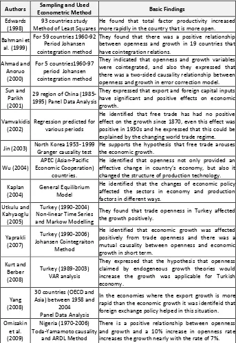
Table 2: Abstract of Empirical Studies Regarding the Openness and Growth
Relationship
Authors Sampling and Used
Econometric Method Basic Findings Edwards
(1998)
93 countries study Method of Least Squares
He found that total factor productivity increased more rapidly in the country that is more open.
Bahmani et al. (1999)
For 59 countries 1960-92 Period Johansen cointegration method
They found that there was a positive relationship between openness and growth in 19 countries that have cointegration relations.
Ahmad and Anoruo
(2000)
For 5 countries1960-97 period Johansen cointegration method
They indicated that openness and growth variables were cointegrated, and also they expressed that there was a two-sided causality relationship between openness and growth in error correction model. Sun and
Parikh (2001)
29 region of China (1985-1995) Panel Data Analysis
They expressed that export and foreign capital inputs have significant and positive effects on economic growth.
Vamvakidis (2002)
Regression predicted for various periods
He identified that free trade has had no positive effect on the growth since 1870, even this effect was positive in 1930s and he expressed that this could be explained by the changing world trade regime.
Jin (2003) North Korea 1953- 1999 Granger causality test
He supports the hypothesis that free trade arouses the economic growth.
Wu (2004)
APEC (Asian-Pacific Economic Cooperation)
countries.
He identified that openness not only provided an effective change in country’s economy, but also it changed the structure of production technology.
Kaplan (2004)
General Equilibrium Model
He identified that the changes of economic policy affected the sectors in economy and production factors in different ways.
Utkulu and Kahyaoglu (2005)
Turkey (1990-2004) Non-linear Time Series and Markow Modelling
They found that trade openness in Turkey affected the growth positively.
Yaprakli (2007)
Turkey (1990-2006) Johansen Cointegraiton
Method
He identified that economic growth was affected positively from trade openness and there was a mutual causality between openness and economic growth in short term.
Kurt and Berber (2008)
Turkey (1989-2003) VAR analysis
They expressed that the hypothesis that openness claimed by endogeneous growth theories would increase the growth was applicable for Turkish economy.
Yang (2008)
30 countries (OECD and Asia) between 1958 and
2004 Panel Data Analysis
In the economies where the export growth is more rapid than the economic growth it was identifeid that foreign exchange policy helped in this situation.
Omisakin et al. (2009)
Nigeria (1970-2006) Toda-Yamamoto causality
and ARDL Method
There is a positive relationship between openness and growth and a 10% increase in openness rate increases the growth nearly with the rate of 7%.
4. Empirical Analysis
4.1. Data Set and Model
In this study, the effect of openness on economic growth was searched for the most rapidly developing countries (emerging markets; Brazil, Russia, India, China and Turkey, BRIC-T) via panel data analysis by using the annual data of the period from 1989 to 2010. From the variables used in the analysis y and open represent the real GDP (constant 2000 US$) and trade openness (export+import/GDP) respectively. The data was obtained from World Bank (www.worldbank.org).
For analysis, Stata 11.0 and Eviews 7 econometric analysis programmes were used and for model choice and correction tests codes were used.
4.2. Method
Panal data analysis was used to search the data from different countries together (Baltagi, 2001; Gujarati, 1999).
=∝ +′ +
(1)
This model is based on decomposing the error term ( ) to its components in terms of its individual and time effects. In the model i indicate the countries, t indicates the time. When the error term is decomposed:
= + + (2)
is obtained. This final equation is called error component model. Here indicates the individual effects, indicates the time effects. It is supposed , ~(0, ) (Independent Identically Distributed), in other words the avarage of error terms is zero, its variance is stationary and it is distributed normally (having white noise process). In the Panel data analysis the stationary of the series are searched through panel unit root tests firstly. Then the type of individual and time effects should be identified. An endogeneity test should be conducted among the variables when there is a variable which is considered to have a close relation with the given variable, therefore it is suspected for its endogeneity. After that a model should be estimated and the problems of heteroskedasticity and autocorrelation in the model should be tested.
4.3. Panel Unit Root Analysis
The first problem in panel unit root test is whether the cross sections building the panel are independent or not. At that point panel unit root tests are classified as the first generation and the second generation. The first generation tests are also classified as homogeneous and heterogeneous. Levin, Lin and Chu (2002), Breitung (2000) and Hadri (2000) are based on homogeneous model hypothesis, whereas Im, Pesaran and Shin (2003), Maddala and Wu (1999), Choi (2001) are based on heterogeneous model hypothesis. On the other hand, the main second generation unit root tests are MADF (Taylor and Sarno, 1998), SURADF (Breuer, Mcknown and Wallace, 2002), Bai and Ng (2004) and CADF (Pesaran, 2006).
Im, Pesaran and Shin (IPS) and Levin, Lin and Chu (LLC) unit root tests will use in this study. These tests:
∆ =∝+ ∑ β ∆Y" + X"′ δ + ε
" &'
( (3)
is based on the model above. Here ∝ ; is error correction term and when |∝ |<1 happens, we understand that the series is trend stationary, on the other hand when |∝ | ≥1 happens, it has unit root, thus it is nonstationary. The tests enable the ∝ to differentiate for the cross section units, in other words heterogeneous panel structure. Tests hypotheses:
H0: ∝ = 1 for all the cross section units, so the series is nonstationary.
H1: ∝ < 1 for at least one cross section unit, so the series is stationary.
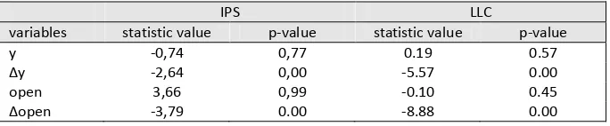
When the probability value obtained from the test results is smaller than 0.05, H0 is rejected and it is decided that the series are stationary. IPS and LLC panel unit root test results are on Table 4.
Table 4: IPS and LLC Panel Unit Root Test Results
IPS LLC
variables statistic value p-value statistic value p-value
y -0,74 0,77 0.19 0.57
Δy -2,64 0,00 -5.57 0.00
open 3,66 0,99 -0.10 0.45
Δopen -3,79 0.00 -8.88 0.00
Note: In Panel unit root test Schwarz criterion is used and lag length is regarded as 1. Δ symbol indicates that the first differences of the variables were taken. As a test style at level value for series trend and intercept regression equation has been used.
4.4. Breush-Pagan Lagrange Multiplier (LM) Test
In this stage of the analysis the LM test was performed in order to determine the type of time effect and individual effects (random or fixed). Because the selected countries aren’t in a certain economic group, it was expected that individual effects would be random and also the time effects of financial development on the growth would be random for the countries in the studied period. Whether or not the effects are really random can be determined with the LM test (Baltagi, 2001:15).
The LM test is classified as LM1 and LM2. LM=LM1+LM2. LM1; tests the individual effects are random and LM2 tests the time effects are random. In LM1 test; H0: -= 0 (no random individual effects) hypothesis is tested through LM1 statistics.
LM1 statistics are calculated with the formula below.
./= 0.2
.(2)3
∑<69:(∑879:4567);
∑<69:∑879:4567; − 1>
(4)
Here, ; indicates the individual effects in the equation (2), N; indicates the cross section (country) number, T; indicates the time dimension, ?; indicates the prediction for the error terms in the equation (1). When the probability value obtained from the test results is smaller than 0.01, H0 is rejected and it is decided that individual effects are random.
In LM2 test; H0: @= 0 (No random time effect) hypothesis is tested by LM2 statistics. LM2 statistics are calculated with the formula below.
./= 0.2
.(0)3
∑879:(∑8<A9:4567);
∑<69:∑879:4567; − 1>
(5)
Here, ; indicates the individual effects in the equation (2), N; indicates the cross section (country) number, T; indicates the time dimension, ?; indicates the predictions for the error terms in the equation (1). When the probability value obtained from the test results is smaller than 0.01, H0 is rejected and it is decided that the time effects are random.
In LM=LM1+LM2 test;
H0: -= @= 0 (no random individual and time effects)
H1: At least one -≠ 0 and at least one @≠ 0 (random effects both).
Table 5: LM Test Results
Test p-value Decision
LM1 0,243 Individual Effects aren’t Random.
LM2 0,052 Time Effects aren’t Random.
LM 0.032 Individual and Time Effects aren’t Random.
Note: 1% significance level was taken.
When we look the results in Table 5, we can see that individual effects, time effects and individual and time effects aren’t random. According to LM test result the estimation was made using the two-way fixed effect model.
4.5. Hausman Endogeneity Test
In this stage of the study, whether there was a relationship between the individual effects and the explanatory variables or not was tested by Hausman method after model estimated with two way random effect model. Test hypotheses:
H0: Cov(, C) = 0 No endogeneity problem.
H1: Cov(, C) ≠ 0 An endogeneity problem.
Here ; indicates the individual effects in the equation (4), but indicates the explanatory variables in the equation (3). When the probability value of D (Chi2) obtained from the analysis is smaller than 0.05, H0 is rejected and it is decided that there is an endogeneity problem in the model. In this case fixed effects model is used (Greene, 2003). However, when H0 is accepted, random effects model is used. This prediction is effective, non-deviated and consistent. Hausman test is not an alternative for LM test. But it functions to check the decision by LM test.
Hausman test was conducted and χ2=14.62 ve χ2 probability value =0.028 was obtained and since this value was smaller than 0.05, H0 hypothesis was rejected and it was decided that there was an endogeneity problem in the model. In this case, it is necessary to do the analysis with the fixed effects model and this result supports the LM test results.
4.6. Two-way Fixed Effects Model Estimations
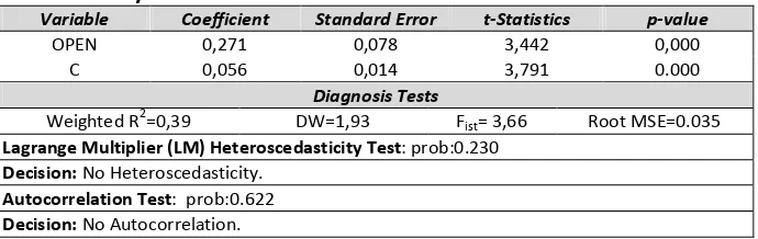
Panel data analysis is estimated by the two-way fixed effect model and the result are on the Table 6.
Table 6: Analysis Results
Variable Coefficient Standard Error t-Statistics p-value
OPEN 0,271 0,078 3,442 0,000
C 0,056 0,014 3,791 0.000
Diagnosis Tests
Weighted R2=0,39 DW=1,93 Fist= 3,66 Root MSE=0.035
Lagrange Multiplier (LM) Heteroscedasticity Test: prob:0.230 Decision: No Heteroscedasticity.
Autocorrelation Test: prob:0.622 Decision: No Autocorrelation.
Conclusion
In this study the effect of trade openness level on economic growth was searched via panel data analysis method in the sample of five developing countries which have an important place in the world economy (emerging markets; Brazil, Russia, India, China and Turkey-BRIC-T). In the study, annual data between 1989 and 2010 periods was used. At the panel unit root analysis result it was found out that series were nonstationary and the effects of shocks on the series did not disappear after a while and therefore it was determined that macroeconomic shocks affected the economy of the countries significantly.
At the LM tests result conducted to define the applicable panel data analysis method, it was found out that individual and time effects weren’t random, for that reason an analysis with the two-way fixed effect model was carried out. At the diagnosis tests result it was found out that there was no heteroskedasticity and autocorrelation problems in the model. In this regard, the estimated model is reliable.
As a conclusion, in the study the effect of trade openness were searched and it was found that openness positive affected the economic growth. If the sustainable growth is considered as one of the most significant macroeconomic variables of the growth for the countries, the increase in foreign trade especially in export are very important.
References
Anorua, E., & Ahmad, Y. (2000). Openness and economic growth: evidence from selected Asian countries. The Indian Economic Journal, 47(3): 110-117.
Bahmani, O. & M., Niromand, F. (1999). Openness and economic growth: an empirical investigation. Applied Economics Letters, 6: 557-561.
Bai J.& Ng S. (2004). A panic attack on unit roots and cointegration. Econometrica, 72: 1127-1178.
Baltagi B. H. (2001). Econometric analysis of panel data. (2d ed). New York: John Wiley & Sons.
Barro, R. J. & Sala-i Martin, X. (1995). Economic growth, McGraw-Hill, Inc., New York.
Breuer B., Mcnown R. & Wallace M. (2002). Series-Specific unit root test with panel data. Oxford Bulletin of Economics and Statistics, 64: 527–546.
Breitung J. (2000). The local power of some unit root tests for panel data. in B. Baltagi (ed.), Nonstationary Panels, Panel Cointegration, and Dynamic Panels, Advances in Econometrics, 15: 161-178.
Chang, H. J. (2004). Kalkınma reçetelerinin gerçek yüzü, (Çev. Tuba Akıncılar Onmuş), İletişim Yayınları, İstanbul.
Choi I. (2001). Unit roots tests for panel data, Journal of International Money and Finance, 20: 229–272.
Chow, P. C. Y. (1987). Causality between exports and industrial development: empirical evidence from the nic's. Journal of Development Economics, 26: 55-63.
Çelebi, Işın (1991). Dışa açık büyüme ve Türkiye, Yayınları, İstanbul.
Dar, A. & Amirkhalkhali, S. (2003). On the impact of trade openness ongrowth: further evidence from OECD countries. Applied Economies, 35(2): 1761-1766.
Dollar, D. (1992). Outward-Oriented developing economies really do grow more rapidly: evidence from 95 LDCs, 1976-1985. Economic Development and Cultural Change, 40: 523– 544.
Edwards, S. (1992). Trade orientation, distortions, and growth in developing countries.
Journal of Development Economics, 39: 31-57.
Edwards, S. (1998). Openness, productivity and growth: what do we really know?. The Economic Journal, 108(March): 383-398.
Frank, W. P. & Frank, E. C. (2010). International business challenge: can the BRIC countries take world economic leadership away from the traditional leadership in the near future?. International Journal of Arts and Sciences, 3(13): 46-54.
Grossman, G. M., & Helpman, E. (1991), Innovation and growth in the global economy, Cambridge, mass. MIT Press.
Gujarati, D. N. (1999). Basic econometrics, McGraw Hill. (3rd Ed.). İstanbul: Literatür Yayıncılık.
Hadri K. (2000). Testing for stationarity in heterogenous panels. Econometrics Journal, 3: 148-161.
Han, E. & A. Kaya, A. (2006). Kalkınma ekonomisi teori ve politika, Nobel Yayın Dağıtım, Ankara.
Harrison, A. (1996). Openness and growth: a time series, cross-country analysis for developing countries. Journal of Development Economics, 48: 419-447.
Im K., Pesaran H. & Shin Y. (1997). Testing for unit roots in heterogenous panels. Mimeo, Department of Applied Economics, University of Cambridge.
Im K., Pesaran H. & Shin Y. (2003). Testing for unit roots in heterogenous panels. Journal of Econometrics, 115: 53–74.
Jin, J. C. (2003). Openness and growth in North Korea: evidence from time-series data. Review of International Economics, 11(1):. 18-27.
Kaplan, M. (2004). An analytical evaluation of the impact of openness on economic performance: a three-sector general equilibrium open economy model. Turkish Economic Association, Discussion Paper, 2004/14, June.
Kurt, S. & Berber, M. (2008). Openness in Turkey and economic growth, Atatürk University Economic and Admisnistritive Journal, 22(2): 57-79.
Kwan, A. C. C., &Cotsomitis, J. (1991). Economic growth and the expanding export sector: China 1952-1985. International EconomicJournal, 5: 105-117.
Levine, R. & Renelt, D. (1992). A sensitivity analysis of cross-country growth regressions.
American Economic Review, 82:, 942-963.
Levin, A., Lin, C. & Chu J. (2002). Unit roots tests in panel data: asymptotic and finite sample properties. Journal of Econometrics, 108: 1-24.
Lucas, Robert; (1988). On the mechanics of economic development”, Journal of Monetary Economics, 22(1): 3-42.
Maddala, G. S. & Wu, S. (1999). A comparative study of unit root tests with panel data and a new simple test. Oxford Bulletin of Economics and Statistics, 61: 631-652.
Omisakin, O., Oluwatosin, A. & Ayoola, O. (2009). Foreign direct investment, trade openness and growth in nigeria. Journal of Economic Theory, 3(2): 13-18.
O’neill, J. (2001), Building better global economic BRICs, Goldman Sachs, Global Economics, Paper No: 66: 1-16.
Pesaran, H. (2006). A simple panel unit root test in the presence of cross section dependence. Cambridge University ,Working Paper, No: 0346.
Rodriguez, F. & Rodrik, D. (1999). Trade policy and economic growth: a skeptic’s guide to cross-national evidence, NBER Working Paper, 7081.
Romer, P. (1986). Increasing returns and long run growth, Journal of Political Economy, 94(5): 1002-1037.
Sachs, J. D. & Warner, A. (1995). Economic reform and the process of global integration.
Brooking Papers of Economic Activity, (1): 195.
Sinha, D. & Sinha, T. (1996). Openness and economic growth: time series evidence from india. Applied Economics: 21-28.
Somel, C. (2009). Economic crises and capital savings. Tes-Iş Journal (March): 80-83.
Sun, H. & Parikh, A. (2001). Exports, inward foreign direct investment (FDI) and regional economic growth in China. Regional Studies, 35 (3): 187-196.
Taylor, M. & Sarno, L. (1998). The behaviour of real exchange rates during the post-bretton woods period. Journal of International Economics, 46:, 281-312.
Turedi, S. & Berber, M. (2010). Finansal kalkınma, ticari açıklık ve ekonomik büyüme arasındaki ilişki: Türkiye üzerine bir analiz. Erciyes University Economic and Admisnistritive Journal, 35(1): 301-316.
Utkulu, U. & Kahyaoğlu, H. (2005). How did the trade and financial openness in Turkey affected the growth?. Turkish Economy Instituation Arguement Text 13, Web; http://www.tek.org.tr/ dosyalar/Utkulu-2005.pdf, Access Date: 11.02.2012.
Vamvakidis, A. (2002). How robust is the growth-openness connection? Historical evidence. Journal of Economic Growth, 7: 57-80.
Wu, Y. (2004). Openness, productivity and growth in the apec economies. Empirical Economies, 29: 593-604.
Yang, J. (2008). An analysis of so-called export-led growth, IMF Working Paper, WP/08/220.