Proc. IAHS, 372, 183–187, 2015 proc-iahs.net/372/183/2015/ doi:10.5194/piahs-372-183-2015
© Author(s) 2015. CC Attribution 3.0 License.
Open Access
v
ention
and
mitigation
of
natur
al
and
anthropogenic
hazards
due
to
land
subsidence
Compaction parameter estimation using surface
movement data in Southern Flevoland
P. A. Fokker1, J. Gunnink1, G. de Lange2, O. Leeuwenburgh1, and E. F. van der Veer1 1TNO, Utrecht, the Netherlands
2Deltares, Utrecht, the Netherlands
Correspondence to: P. A. Fokker ([email protected])
Published: 12 November 2015
Abstract. The Southern part of the Flevopolder has shown considerable subsidence since its reclamation in 1967. We have set up an integrated method to use subsidence data, water level data and forward models for com-paction, oxidation and the resulting subsidence to estimate the driving parameters. Our procedure, an Ensemble Smoother with Multiple Data Assimilation, is very fast and gives insight into the variability of the estimated parameters and the correlations between them. We used two forward models: the Koppejan model and the Bjer-rum model. In first instance, the BjerBjer-rum model seems to perform better than the Koppejan model. This must, however, be corroborated with more elaborate parameter estimation exercises in which in particular the water level development is taken into account.
1 Introduction
The Southern part of the Flevopolder (the Netherlands) was reclaimed in 1967–1968. After lowering the groundwater level, the sediments compacted, resulting in surface subsi-dence. The compaction is a combination of elastic and vis-coplastic compaction of clay and peat, and of peat oxidation. A good prediction of future compaction and an extrapolation to other areas naturally requires knowledge of the subsurface lithology, the compaction parameters and the phreatic wa-ter level development. The present paper describes an exer-cise of parameter estimation using a limited number of bore-hole data in the Southern Flevopolder area. An Ensemble Smoother with Multiple Data Assimilation was employed to this end.
2 Available data
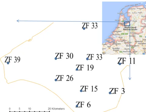
The Flevopolder is a large polder in the Netherlands, which was reclaimed from the IJsselmeer in 1967 (Fig. 1). The sur-face has an elevation of about 3 m below sea level. The com-position of the subsurface had been mapped on a number of places prior to the reclamation. It is a variable layered struc-ture which we categorized into four generic types: clay, hu-mic clay, peat, and sand. For the present study, 10
measure-ment locations were selected, at which the surface level had been monitored yearly between 1967 and 1993 by geodetic levelling.
Data about the phreatic groundwater level are scarce. One of the few measurements covering the complete period is rep-resented in Fig. 2. It shows the fast lowering of the water level at reclamation of the polder, followed by a gradual decrease during the next 7 years. This can be explained by the gradual adjustment of the phreatic level at the measurement location to the drainage level in the ditches.
3 Forward model
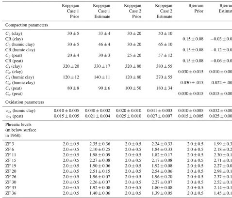
Table 1.Assimilation results.
Koppejan Koppejan Koppejan Koppejan Bjerrum Bjerrum
Case 1 Case 1 Case 2 Case 2 Prior Estimate
Prior Estimate Prior Estimate
Compaction parameters
Cp(clay) 30±5 33±4 30±20 50±10
CR (clay) 0.15±0.08 −0.03±0.06
Cp(humic clay) 30±5 46±4 30±20 65±10
CR (humic clay) 0.15±0.08 −0.12±0.05
Cp(peat) 20±4 30±3 25±20 57±12
CR (peat) 0.15±0.08 −0.06±0.04
Cs(clay) 320±20 330±17 320±80 380±55
Cα(clay) 0.030±0.015 0.010±0.005
Cs(humic clay) 120±12 140±11 120±80 270±55
Cα(humic clay) 0.030±.015 0.022±.009
Cs(peat) 80±8 90±6 100±50 180±34
Cα(peat) 0.030±0.015 0.015±0.008
Oxidation parameters
νox(humic clay) 0.010±0.005 0.030±0.002 0.020±0.010 0.041±0.003 0.010±0.005 0.032±0.002
νox(peat) 0.015±0.005 0.021±0.004 0.025±0.010 0.027±0.007 0.015±0.005 0.025±0.003
Phreatic levels (m below surface in 1968):
ZF 3 2.0±0.5 2.35±0.36 2.0±0.5 2.24±0.33 2.0±0.5 1.99±0.35
ZF 6 2.0±0.5 2.10±0.25 2.0±0.5 1.84±0.33 2.0±0.5 2.18±0.25
ZF 11 2.0±0.5 1.98±0.09 2.0±0.5 1.82±0.17 2.0±0.5 2.30±0.19
ZF 15 2.0±0.5 2.27±0.08 2.0±0.5 2.17±0.08 2.0±0.5 2.71±0.11
ZF 19 2.0±0.5 1.90±0.06 2.0±0.5 1.92±0.08 2.0±0.5 2.27±0.09
ZF 20 2.0±0.5 2.51±0.15 2.0±0.5 2.54±0.06 2.0±0.5 2.98±0.19
ZF 26 2.0±0.5 1.96±0.07 2.0±0.5 1.96±0.20 2.0±0.5 2.37±0.10
ZF 30 2.0±0.5 2.26±0.07 2.0±0.5 2.27±0.07 2.0±0.5 2.52±0.11
ZF 33 2.0±0.5 1.92±0.08 2.0±0.5 1.80±0.08 2.0±0.5 2.14±0.10
ZF 36 2.0±0.5 1.40±0.06 2.0±0.5 1.39±0.05 2.0±0.5 1.45±0.12
subsidence as a function of time:
εv,Koppejan= 1
Cp
+ 1 Cs
log t
tref
×lnσ
0
σ00+
1−exp (−voxt)
εv,Bjerrum=CR log
σ0
σ00+Cαlog t tref
+1−exp (−voxt)
Here, σ0 andσ00 are the actual and original effective verti-cal stresses;CpandCsare the primary and secondary
com-pression coefficients above pre-consolidation pressure in the Koppejan model; vox is the oxidation rate; CR andCα are
the virgin compressibility (above pre-consolidation pressure) and the creep parameter or coefficient of secondary compres-sion in the Bjerrum model.
4 Inverse model
The present study aimed at the assessment of the uncer-tainty of the model parameters in order to improve the
his-tory match of the ground level displacement and the reliabil-ity of the associated predictions. We considered as uncertain parameters the primary and secondary compression coeffi-cients, the oxidation rates and the phreatic water levels. We assumed the measured lithology at every location as fixed. Of the four lithologies identified, we assumed the sand to be incompressible. Both models were thus left with 18 uncer-tain parameters: primary and secondary creep parameters for clay, for humic clay, and for peat (6 parameters); oxidation rates for humic clay and for peat (2 parameters); and ground-water levels for each location (10 parameters).
We define the vector m as the collection of adjustable model parameters; the vectordas the collection of data (sur-face level measurements vs. time) and the functionalG(m), working on the model parameters, as the forward model. The inverse problem is then formulated as the task of estimating the vectormfor whichG(m) approaches the data vectord
Figure 1.Map of the SE Flevopolder with the selected locations.
prior model (m0) and covariance matrices of the
measure-ments (Cd) and of the prior model (Cm), the conventional
least-squares solution is obtained by maximizing the objec-tive functionJ given by Tarantola (2005) (or by minimizing the exponent in the expression,−log(J)):
J =exp
−1
2(m−m0)
TC−1
m (m−m0)−
1
2(d−G(m))
T
C−d1(d−G(m))i.
We used an ensemble approach in which the mean and the covariance of the model vector m0 are mapped on an
en-semble of Ne vectors. Different approaches exist to obtain
an estimate of the model vector. A global update of the model using all available data can be achieved in a single step; this procedure is called an Ensemble Smoother (Em-erick and Reynolds, 2012) – it is, however, suboptimal for non-linear problems as ours. When both data and parame-ters are assimilated to newly incoming data in subsequent time steps, the procedure is called a filter. EnKF is an ex-ample of a filter, but we did not use EnKF because all data were available at all times. Emerick and Reynolds (2013) and Tavakoli et al. (2013) state that the best approach for non-linear systems such as ours is to use an Ensemble Smoother with Multiple Data Assimilation (ES-MDA). In ES-MDA, the ensemble smoother is applied iteratively multiple times. In this way, correlations between parameters that result from the smoother are retained in subsequent steps. The advantage of ES-MDA above EnKF is that the data are used as given and that the procedure is computationally less demanding.
5 Results
The results of the estimation exercise with both models are presented in Table 1. For the Koppejan model we report
re-sults that were achieved after starting from two initial distri-butions – the first one with closer bounds than the second.
The results show that the main adjustments for the Koppe-jan model are in the oxidation rates and in the phreatic wa-ter levels. These paramewa-ters have the largest impact on the surface movement rates. The adjustments of the oxidation rates are larger for the less constrained case, as should be expected. For the phreatic water levels, the adjustments are similar. There is quite a large variability in the resulting esti-mate of the phreatic water level among the different locations – this is related to the types of lithology present around the phreatic water level: peat oxidation has the largest influence on subsidence and boreholes with peat will result in a better constrained water level because the sensitivity to it is larger.
For the Bjerrum model, the largest effect is also related to the peat oxidation rates and the water levels, but the com-paction parameters are also significantly constrained. For these parameters, the values of CR andCαare anti-correlated
– an increase in one of them can be partially compensated by a decrease in the other.
Figure 3 visualizes the data, the priors and the inversion results. While a large degree of scatter is present for the prior distribution of parameters, the smoother succeeds in con-straining this uncertainty and obtaining a reasonable fit to the data. The assimilation is better when using the Bjerrum model.
6 Discussion
We wish to address some issues here that are striking from the results as presented above. The first is the relative insen-sitivity to the compaction parameters in the Koppejan model; the second is the appearance of unphysical negative num-bers for the immediate compaction parameter CR in the Bjer-rum model; the third is the high oxidation rates resulting for the humic clay and for the peat – the former even being the largest. In our opinion, these issues are related to a fourth issue: the fact that the match of the curves using estimated parameters is suboptimal in the first 6 or 7 years. We feel there is a strong relation with the fact that the parameter esti-mation with the present dataset was accomplished under the assumption of an immediate drop of the water level to a fur-ther constant value. This is a simplification that must be ad-dressed in a follow-up study. Although only limited data on the water level are available, Fig. 2 shows that this assump-tion is not generally applicable. A first-order approximaassump-tion could be to distribute a 1 m level drop to the final value over the first 7 years after reclamation. We are currently building such an extension into our models.
7 Conclusions
Figure 2.Hydraulic head in well B26E00030001, located on the boundary between the previously reclaimed Eastern Flevoland polder and the subsequently reclaimed Southern Flevoland polder. The reclamation of the Southern Flevoland polder in 1967 is followed by a gradual decrease of the level during approximately 7 years; after which the level remains virtually constant until 1995.
Figure 3.Surface movement data and predictions before and after data assimilation. Subsequent series are shifted downward by 0.5 m. Colored circles: data; colored dashed lines: average prior estimate; colored solid lines: average assimilated estimate. Light grey lines: prior ensemble predictions. Dark grey lines: posterior ensemble predictions. Case 2, with less constrained prior gives larger prior spread and better estimates than Case 1.
and phreatic water levels for 10 locations in the Southern Flevopolder, using surface movement parameters between the moment of reclamation in 1967 and 1993. The proce-dure, using an Ensemble Smoother with Multiple Data As-similation, is very fast and gives insight into the variability of the estimated parameters and the correlations between them.
References
Bjerrum, L.: Engineering geology of Norwegian normally con-solidated marine clays as related to settlements of buildings, Géotechnique, 17, 81–118, 1967.
Emerick, A. and Reynolds, A. C.: Ensemble smoother with multiple data assimilation, Comput. Geosci., 55, 3–15, 2012.
Emerick, A. and Reynolds, A. C.: Investigation of the sampling performance of ensemble-based methods with a simple reservoir model, Comput. Geosci. 17, 325–350, 2013.
Koppejan, A. W.: A Formula Combining the Terzaghi Load Com-pression Relationship and the Buisman Secular Time Effect, Proc. Int. Conf. Soil Mech. Found. Eng., Rotterdam, 3, 32–38, 1948.
Tarantola, A.: Inverse Problem Theory and Methods for Model Pa-rameter Estimation, SIAM, Paris, France, 2005