SLOPE-BASED PATH SHIFT PROPENSITY ALGORITHM FOR THE STATIC TRAFFIC ASSIGNMENT PROBLEM

SLOPE-BASED PATH SHIFT PROPENSITY ALGORITHM FOR

THE STATIC TRAFFIC ASSIGNMENT PROBLEM

Amit Kumar1_{, Srinivas Peeta}2

1 _{NEXTRANS Center, Purdue University, West Lafayette, IN, USA} 2 _{School of Civil Engineering, Purdue University, West Lafayette, IN, USA}

Received 16 June 2014; accepted 20 July 2014

Abstract: This paper presents a path-based traffic assignment algorithm for solving the static deterministic user equilibrium traffic assignment problem. It uses the concepts of the path shift-propensity factor and the sensitivity of path costs with respect to path flows in the flow update process, and is labeled as the slope-based path shift-propensity algorithm (SPSA). It seeks to enable faster convergence, incorporates behavioral realism in the flow update process, and maintains simplicity of execution for easy deployment in practice. The behavioral rationale behind the proposed algorithm is explained. The mathematical exposition of the algorithm and its proof of convergence are articulated. Numerical experiments are conducted using test networks to benchmark the performance of SPSA. The computational performance of the SPSA is compared with those of two versions of the recently developed path-based algorithm labeled slope-based multipath algorithm (SMPA), the widely-used Frank-Wolfe (F-W) algorithm, and a variant of the F-W algorithm labeled the social pressure algorithm (SPA). They illustrate that the rate of convergence of the SPSA is very close to that of the SMPA and significantly better than those of the F-W algorithm and the SPA. One version of the SMPA performs better than the SPSA in terms of convergence, though the latter is easier to implement and hence a potential substitute for SMPA in practice. Further, the results vindicate the notion that the SPSA is a feasible deployment option under the computational capabilities available today.

Keywords:traffic assignment, user equilibrium, path flows, path shift-propensity.

1 _{Corresponding author: [email protected]}

1. Introduction

The traffic assignment problem (TAP) has been extensively studied for over five decades, and many approaches and algorithms have been developed to solve it and its variants. Due to its relevance to practice, the most commonly solved problem in this context is the static deterministic user equilibrium problem,

The UETAP can be formulated as a convex optimization problem with a non-linear objective function and a set of linear constraints (Beckmann et al., 1956). This formulation yields a unique solution in terms of link flows under the assumption that the link performance functions are separable, continuous and strictly monotonically increasing. However, while link f lows are unique, path flows are non-unique as multiple solutions in terms of path flows can represent the same link flows. This non-uniqueness is an inherent property of all networks having the number of possible paths larger than the sum of the number of links and origin-destination (O-D) pairs (Lu and Nie, 2010). There have been some recent efforts to uniquely obtain the path flows under some additional conditions. One such condition is based on the principle of entropy maximization (Rossi et al., 1989; Bar-Gera, 2010), though the authors themselves have questioned the realism of these approaches relative to real-world traveler behavior. Hence, the need for real-world reliability of path-based solutions entails developing models that can more realistically represent the equilibration process. In addition to this, faster and smoother convergence and simplicity of execution are other desirable properties for the applicability of a method in practice. In practice, the iterative UETAP solution procedure is typically terminated, though not justifiably, at an arbitrary point due to computational time constraints. If the iterations in the solution procedure illustrate significant oscillations, issues of confidence in the solution obtained arise under arbitrary termination. This issue can be circumvented through approaches that ensure smoother convergence.

Kumar and Peeta (2010) developed a path-based algorithm labeled the

slope-based multi-path algorithm (SMPA) for the UETAP, aimed at achieving smoother and faster convergence. SMPA uses the sensitivity of the path cost with respect to flow in the form of the slopes of the path cost functions, avoids the line search by using a constant value of scaling factor and updates the flows of paths between an O-D pair simultaneously to achieve smoother and faster convergence. However, a practical issue is that its execution requires the calibration of two parameters which requires multiple runs of the algorithm. These parameters have no upper bound and the performance of the SMPA is very sensitive to these parameters. Hence, the SMPA performance depends on the precision in calibrating the optimal values of parameters. In addition, it is relatively complex to implement compared to the well-known Frank-Wolfe (F-W) algorithm. This motivates the current study which seeks to develop a solution algorithm for the UETAP that inherits the merits of the SMPA, tends to robustly incorporate real-world traveler behavior in the flow update process, and maintains the simplicity of execution for practice.

to minimum path costs. However, there are two potential conceptual gaps related to this algorithm, which when addressed can lead to further realism in the flow update process, representing another key motivation for the current study. First, the SPA implies that drivers from all costlier paths will shift to a single path with minimum cost though other potentially attractive paths exist with costs close to or even equal to the minimum cost. Second, the move direction of the SPA ignores the sensitivity of the path cost to the path flow. This implies that drivers will shift to a minimum cost path from multiple paths irrespective of the increase in congestion due to these shifts. Both these issues are problematic from a realism viewpoint. The SPSA inherits insights from both the SPA and the SMPA, and seeks to bridge the conceptual gaps in the SPA by enabling flow shifts to multiple potentially attractive paths. It also utilizes the sensitivity of path costs in the form of the slopes of the cost functions to add more behavioral realism, and also achieve smoother and faster convergence. The mathematical derivations of the move direction for the SPSA, and its proof of convergence, are provided in section 4 of this paper.

The remainder of the paper is organized as follows. The section 2 summarizes the related literature in this domain. Then, the formulation of the UETAP problem is presented in section 3. Section 4 presents the mathematical derivation of the SPSA algorithm along with its proof of convergence. Then, the results of computational experiments are illustrated in section 5, that compare the relative performance of the SPSA with SMPA, SPA and Frank-Wolfe algorithm. Finally, some concluding comments are presented in section 6.

2. Literature Review

The idea of equilibrium in traffic flows originated in 1924 when economist Frank Knight proposed “Social Cost,” to explain how the truck operators will tend to distribute themselves between various roads if they are tolled (Knight, 1924). This idea was formalized in the form of two principles by John Wardrop; they form the basis for analyzing traffic equilibrium and are labeled as Wardrop’s first and second principles (Wardrop, 1952). Beckmann et al. (1956) proposed the UETAP as an optimization problem, which is known as Beckmann’s transformation. In the same year, the linear approximation method was devised by Frank and Wolfe to solve the quadratic problem, which is known as the Frank-Wolfe (F-W) algorithm. This method was adopted to solve the network equilibrium problem by Bruynooghe et al. (1969), and later by LeBlanc (1973) and LeBlanc et al. (1975) and Nguyen (1974). Florian and Nguyen (1976) and Dow and Van Vliet (1979) provided the validation studies for this method, and it was adopted as the technique for solving UETAP in related commercially developed software. Since then, the F-W algorithm has been the most commonly used method, which replaced the heuristic methods (Sheffi, 1985) that were previously used in practice.

perpendicular to the direction of maximum descent near convergence. This deficiency has lead to many variants of F-W algorithm. Most of these have attempted to modify the step size or search direction. Weintraub et al. (1985) suggested the use of a modified step size which is obtained by multiplying the optimal step size by some factor to reduce the zigzagging effect in the F-W algorithm. Other such examples include the methods suggested by Wolfe (1970) and Meyer (1974). Luenberger (1973) suggested an improved F-W algorithm by using the parallel tangent (PARTAN) direction which was introduced in the TAP by LeBlanc et al. (1985) and Florian et al. (1987). Fukushima (1984) suggested a method that uses the convex combination of linear program solutions from previous iterations to generate a new search direction. Then, the directional derivatives of this new search direction and the F-W search direction are computed, and the search direction with the lower directional derivative among these two is used to generate the next updated solution. Lee and Nie (2001) proposed a method similar to Fukushima, but use a heuristic to determine parameters for modifying the search direction based on the congestion levels in the network. Most of these methods operate in the space of link flows and benefit from the basic structure of the F-W algorithm which requires lesser memory usage.

Over time, the need for path-based solutions was felt by planners, and led to the re-visit of the path-based method which was first proposed by Dafermos (1968) and Dafermos and Sparrow (1969). This method equilibrates a single origin-destination (O-D) pair at a time, by shifting flows from the longest path to the shortest path at each move. The step size for each move is obtained through a line search

projected gradient method of Rosen (1960) which also provides a solution in terms of path flows and equilibrates one O-D pair at a time sequentially. This algorithm uses the average cost for finding the search direction and does not require the second derivative information. Recently, Kumar and Peeta (2010) developed an algorithm labeled the slope-based multi-path algorithm (SMPA) that uses the slope of the cost function efficiently to shift flows from the set of costlier paths to the set of cheaper paths simultaneously and seeks to move path costs towards the average cost for an O-D pair at each iteration to achieve faster convergence.

There is another type of algorithm which is based on modifying the search direction of the F-W algorithm but operates in the space of path flows. The social pressure algorithm developed by Kupiszewska and Van Vliet (1998) lies under this category. It retains the simple structure of F-W algorithm but improves the rate of convergence by using a social pressure factor. The concept of social pressure used in this algorithm has behavioral consistency with the likely rationale used by network users to seek better paths. It states that the number of users who shift from a costlier path is proportional to the difference of the cost on that path from that of the minimum cost path. The SPSA algorithm proposed in this paper leverages this concept and insights from the SMPA algorithm in deriving its search direction and endeavors to overcome the demerits of both of them. The key difference is that unlike SMPA it does not require calibration of multiple parameters and unlike SPA it entails flow shifts to multiple attractive paths and uses the sensitivities of the path costs with respect to flow while shifting flows;

this enhances behavioral realism in the flow update process as explained later in sections 4.1 and 4.4.

3. Problem Formulation and Notation

Let the network of interest be represented by a set of nodes N, and a set of links A. Let

R and S, respectively, be the set of origin and destination nodes which may not be mutually exclusive. The set of feasible paths that connect an O-D pair r-s is denoted as Krs _and the O-D demand as qrs. Let xa and ca represent the flow and cost on link a respectively, and

fkrs and ckrs represent the flow and cost on path

k of O-D pair r-s, respectively. The cost of traveling on a path is equal to the sum of the costs on the links of that path, where the link cost is a function ca(xa) of the flow on that link. The UETAP can be represented as an optimization problem using the well-known Beckmann’s transformation (Beckmann et al., 1956) which has a minimization objective function:

0

min

( )

xa _a

( )

a A

Z x

c w dw

∈

=

∑∫

(1)

subject to constraints on flow conservation, non-negativity, and link-path incidence definition, as follows:

,

rs

k rs

k

f

q

rs

=

∀

∑

(1a)

0, ,

rs

k

f

≥

∀ ∀

k rs

(1b)

,

, 1

, if link lies on path , 0 otherwise rs rs rs

a k a k a k

r s k

a k

x

=

∑∑∑

f

δ

δ

=

(1c)

In addition to the basic assumptions of user equilibrium which assumes familiarity of all network users with the network and their homogenous rational behavior, the equivalency of this formulation to the static UE problem and the uniqueness of the solution in terms of link flows requires following assumptions: (i) O-D demand is constant and non-negative for all O-D pairs, (ii) link costs are positive and strictly monotonically increasing, and continuously differentiable functions of flow, and (iii) the link cost depends only on the flow on that link and does not depend on the flow on other links. Under these assumptions, the Hessian matrix of the objective function is a diagonal matrix with positive diagonal elements, and is positive definite. Then, the solution of above problem in terms of link flows is unique but not so in terms of path flows. User familiarity with a network implies that the network users are familiar with the network topology and travel times. The network familiarity in this study also implies that users know the sensitivity of path cost with respect to flow based on repeated travel experiences.

4. SPSA Algorithm Development

This section reviews the flow update process of F-W algorithm and SPA along with their limitations and conceptual gaps and explains how those conceptual gaps are bridged in SPSA. The path-based UETAP problem formulation is presented to represent the equilibration process of SPSA. Then the derivation of the mathematical expression for the move direction of SPSA along with the proof of convergence and implementation details is presented.

4.1. Conceptual Basis for the SPSA

The optimization problem represented by Eq. (1) in the previous section is solved using an iterative flow update process, where the move direction at each iteration seeks to decrease the value of the objective function. The iterative process terminates when the convergence criterion is met. In the F-W algorithm, this link-based f low update process at any iteration n is (Sheffi, 1985):

1

₍

₎

n n n n

a a n a a

x

+

₌

x

₊

λ

y

₋

x

(2)

where,

x

_an+1is the updated link flow on link a, which is the combination of present link flow

n a

x and the auxiliary link flow yanobtained

by assigning the entire demand for each O-D pair to its current shortest path (that is, an all-or-nothing (AON) assignment). λn is

the step size which lies between 0 and 1 and is obtained through a line search procedure that minimizes the value of Z(x). Translating this in terms of a path-based approach, the flow update process for the F-W algorithm can be represented as (Kupiszewska and Van Vliet, 1998):

, *

, 1

, *

(1 )

(1 )

rs n rs n n k k rs n

n k n rs

f if k k

f

f q if k k

λ

λ λ

+ _{= } − ≠

− + =

 (3)

where,

k

*is shortest path, and rs n, 1

k

f + _is

the new flow for path k between the O-D pair r-s for iteration n, which is obtained by combining the present flow rs n,

k

f

and the

require path information from previous iterations. Hence, the memory requirement for this algorithm is low, representing an advantage over path-based algorithms in the past when computers were constrained by their lower memory. But this advantage also implied several limitations to the algorithm. As the path information is lost across iterations, the (link-based) results of the assignment cannot be used for applications which require path information. By using insights from Eq. (3), the flow update process of the F-W algorithm implies that the flow is transferred from non-shortest paths to the shortest path in each iteration. But this flow transfer is proportional to step size

λ

n

, which is uniform for all the non-shortest paths and also for all the O-D pairs. This makes the F-W algorithm insensitive to the cost difference between paths as it shifts a uniform proportion of flow using a single value of step size

λ

n. This is problematic

from a behavioral realism viewpoint, as the fraction of drivers who will shift from a costly path to cheaper path will vary with the path, and will not necessarily be constant across all paths and all O-D pairs. Drivers using more expensive paths compared to the minimum cost path will be more inclined to shift their paths than less expensive paths. Accordingly, larger fractions of drivers traveling on more expensive paths will shift paths than on less expensive paths. Hence, in order to represent this behavioral realism in the flow update process, paths which have lesser cost difference from the minimum cost path will require a smaller value of

λ

_n and paths which have larger cost difference will require a larger value of

λ

n. From a computational

viewpoint as well, using a uniform step size drives the paths that are near minimum cost beyond it by shifting more than required flow, while at the same time this step size may

be insufficient for paths far from minimum cost. Consequently, flow transfer starts oscillating between the paths of an O-D pair, especially near convergence, leading to the poor performance of the F-W algorithm. The social pressure algorithm (Kupiszewska and Van Vliet, 1998) was devised to overcome this drawback.

The social pressure concept is based on the idea that drivers traveling on relatively expensive paths are more strongly inclined to shift paths than those with travel times closer to the minimum cost paths. The social pressure factor (Kupiszewska and Van Vliet, 1998) for a path is defined as the difference of cost of the path from the minimum cost for the O-D pair. In this paper, it is termed as the “path shift-propensity factor” to link it to the real-world meaning, mathematically:

min rs rs rs

k

c

k

c

ρ =

−

(4)

where,

ρ

krsis the path shift-propensity factor

for path k,

c

krsis the cost of path k and

c

minrs

is cost of the shortest path between an O-D pair r-s. In the social pressure algorithm, the step size in the flow update process is weighted by the path shift-propensity factor:

, *

, 1

, , *

(1 rs) rs n n k k rs n

rs n rs rs n k

k n l l l k

f if k k f + _f λ ρ_{λ ρ f if k k}

≠

 − ≠



=  _{+ =}



∑

(5)

where,

λ

nis the step size whose optimum

value minimizes the objective function

Z.

λ

nis not bounded between 0 and 1,

and is constrained by the limits 0 and

max 1/ max( )

rs k

λ =

ρ

. In this method, the

by Eq. (5). This enables the social pressure algorithm to have a more stable as well as faster convergence compared to the traditional F-W algorithm. However, as mentioned earlier in the paper, there are two important deficiencies in this algorithm. First, it transfers flow from all expensive paths to just one shortest path though other paths may exist with cost equal to or very close to the shortest path. This is problematic from both behavioral realism and computational viewpoints. In reality, it is unlikely that drivers will shift from all expensive paths to just one path, and are more likely to shift to various potentially attractive paths which have cost equal to or close to minimum cost for the O-D pair. From a computational perspective, shifting flows from multiple paths to a single path may over-congest that path making it an expensive path in the next iteration. Second, it does not take into account the sensitivity of path costs with respect to flow. Kumar and Peeta (2010) have shown that the efficient use of the slopes of the cost function and the transfer of flows from multiple expensive paths to multiple cheaper paths in the SMPA algorithm lead to faster convergence. The

SPSA is derived by inheriting insights from the SMPA and social pressure algorithms in the flow update process.

4.2. Representation of UETAP from the

Perspective of Path Flows

T he SPSA is based on Gauss-Seidel decomposition techniques where O-D pairs are equilibrated one at time in a sequential order. Let us consider an intermediate stage of the equilibration process at iteration n where an O-D pair r-s is being equilibrated. As the UE conditions are not satisfied, paths with non-zero flows will not have equal cost for an O-D pair. Let Krs _{be the set of feasible paths} between the O-D pair r-s which has unequal cost. Now, using the insights from the SMPA algorithm, the set of feasible paths is divided into two subsets: the set of costlier paths and the set of cheaper paths. Then, the flow is transferred from the set of costlier paths to the set of cheaper paths. This facilitates the flow shift from expensive paths to multiple potential paths. To enable this in the SPSA, the objective function during the equilibration process for an O-D pair r-s is decomposed into three parts:

( )

)

0 0 0

\(

\

( ) ( ) ( ) ( )

rs rs rs rs rs

a a a a a a

x x x x x x

a a a

a P P a P a A P P

Z x −∆ c w dw + ∆ −∆ c w dw c w dw

∈ ∈ ∈

+ +

=

∑

_∫

∑

_∫

∑

_∫



(6)

where:

rs

P = set of cheaper paths, comprising of paths having cost less than or equal to the threshold value_πrs_{for the O-D pair}

r-s, _Prs = set of costlier paths, comprising of paths having cost greater than the threshold value

rs

π for the O-D pair r-s, ∆xa= change in flow

for link a due to flow update of paths in the costlier set,∆xa= change in flow for link a

due to flow update of paths in the cheaper set

process. An iteration is completed when all O-D pairs are equilibrated once. This process is repeated until the convergence criterion is satisfied.

Although above mentioned flow shifts from multiple costlier paths to multiple cheaper paths in SPSA is based on the insights from SMPA, there lies a conceptual difference between them. While in SMPA the threshold value _πrs_{that demarcates the boundary}

between costlier and cheaper paths is equal to average cost of the O-D pair, in SPSA it is obtained using the proximity parameter

δ as below:

min max( ), 0 1

rs rs rs

k

c

π

= +

δ

ρ

≤ <

δ

The prox imit y parameter δ sets the indifference band near minimum cost path by specifying the threshold value

rs

π _{between the maximum cost path and}

minimum cost path. While the value of _πrs

changes from one O-D pair to another and with the iterations as the value of maximum path shift-propensity factor changes, the value of δ remains constant throughout the execution of the algorithm. The value of δ

needs to be calibrated before using SPSA for better performance which was found to be 0.15 and 0.2 for the test networks as shown in section 4.6. In reality, drivers are likely to shift from expensive paths to the paths having cost closer to minimum cost paths and not to all paths having cost less than the average cost. Hence SPSA represents better behavioral realism in its flow update process compared to SMPA. The superscript for O-D pair r-s is dropped hereafter for simplicity of notation as we focus on an O-D pair r-s.

4.3. Derivation of the Move Direction of

SPSA

As explained in section 4.2, the set of feasible paths is divided into two subsets,P(set of cheaper paths) and P(set of costlier paths). The flows are shifted from the set of costlier paths to the set of cheaper paths in proportion to the path shift-propensity factor:

1

₍₁

_{) ,}

n n n

n

k k k

f

+

_{= −}

λ ρ

f

_{∀ ∈ ∈}

k P K

₍₇₎

where,

1 n k

f

+

= new flow on path k belonging to the setPat iteration n

n k

f

= current flow on path k belonging to the setPat iteration n

n k

ρ

_{= path shift-propensity factor for path k}

belonging to the set Pat iteration n

From Eq. (7), we obtain:

1

₍

₎

n n n n

k k k n k k

f

f

f

+

λ ρ

f

∆ =

−

=

(8)

The superscripts n and n+1 are dropped hereafter for simplicity of notation as we focus on an O-D pair r-s at iteration n. Rewriting Eq. (8) we obtain:

(

)

k k k

f

λρ

f

∆ =

(8a)

Assuming that change in path flows are small relative to path flow, new path costs can be expressed as the function of new flows using the first order Taylor expansion:

l( l l) l( )l l( ). , l

c f + ∆f =c f +s f ∆f ∀ ∈ ∈l P K ₍₉₎

where,

l

c

= cost of path l belonging to the setP

l

f = flow of path l belonging to the setP

l

s

= first derivative of the cost function of path l belonging to the setP

Flows are added to paths in the cheaper set such that the increases in the costs of all the paths in this set are equal so as to keep their costs close to each other. Let us assume that new path costs resulting from the new flows are higher than the old path costs by an equal amount

∆

c

. From Eq. (9), we obtain:

l( l l) l( )l l( ).l

c c f f c f s f f

∆ = + ∆ − = ∆ (10)

Rewriting Eq. (10), we obtain:

( )

l l l

c

f

s f

∆

=

_(10a)

The value of ∆c remains constant over the paths in the cheaper set for an O-D pair. The behavioral interpretation of Eq. (10a) is that the higher the sensitivity of the travel cost of a cheaper path with respect to the congestion level, the lower is the proportion of network users shifting to that path from the costlier paths for the O-D pair. This is consistent with the assumption that the user familiarity with the network implies their familiarity with the sensitivity of the path costs with respect to the congestion level.

To satisfy the flow conservation for the O-D pair, the sum of flow transferred from the various paths of setPshould be equal to the sum of flows being added to the paths set

P. Hence,

k l

k P l P

f

f

∈ ∈

∆ =

∆

∑

∑

(11)

Using Eqs. (8a), (10a), and (11), we obtain:

( )

k k

k P l P l l

c

f

s f

λρ

∈ ∈

∆

=

∑

∑

1

( )

k k

l P l l k P

c

f

s f

λρ

∈ ∈

⇒ ∆

∑

=

∑

1

( )

k k k P l P l l

f

c

s f

λρ

∈ ∈

⇒ ∆ =

∑

∑

Substituting the value of

∆

c

back into the Eq. (10a), we obtain:

1

( )

( )

k k k P l

l l _{l P}

l l

f

f

s f

s f

λρ

∈ ∈

∆ =

∑

∑

(12)

Hence, the move direction for the flow update process in the SPSA is:

( ) , , 1 ( ) ( )

k k k

k k k P l

l l l P l l

f f k P

f

f l P

s f s f λρ λρ ∈ ∈  ∆ = ∀ ∈   ∆ = ∀ ∈  

∑

The flows of paths in the feasible set for each O-D pair are updated by using the following flow update mechanism in each iteration:

,

(A)

(B)

k k

l l l

f

f

f

k P

f

f

f

l P

→

− ∆

∀ ∈

→

+ ∆

∀ ∈

,

(A)

(B)

k k

l l l

f

f

f

k P

f

f

f

l P

→

− ∆

∀ ∈

→

+ ∆

∀ ∈

4.4. The Logic of the Flow Update

Mechanism of SPSA

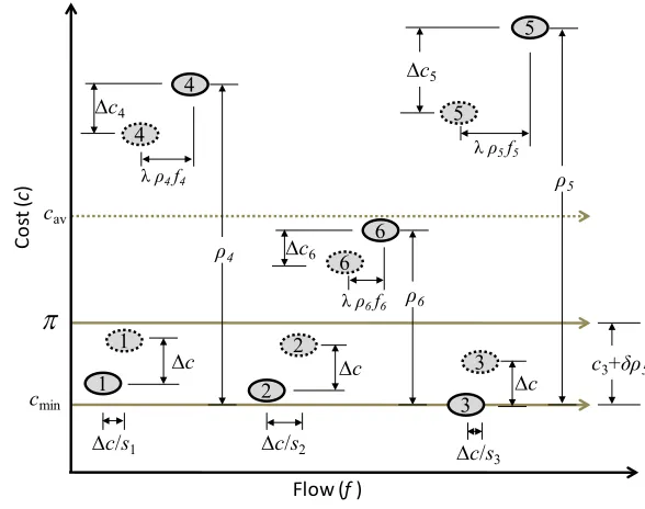
The logic of the proposed f low update mechanism for the SPSA is presented in Fig. 1. To understand the concept, let us assume that the O-D pair which is being updated has six paths in the feasible set, labeled 1 to 6. The current positions of the paths on the flow-cost plot are shown as solid ellipses, and the dotted ellipses show their positions after the flow update. The path labeled 5 has the highest cost and path labeled 3 has the lowest cost. Hence, the maximum path shift-propensity factor for this O-D pair will be equal to the difference of costs of these two paths. Let δ be the predefined proximity parameter; then, the threshold limit (π) is equal to the sum of the cost on path labeled 3 and δ times the path shift-propensity factor of the path labeled 5 as shown in Fig. 1. A path which has cost less than or equal to this threshold value π will fall into the cheaper set and rest of the paths in the feasible set will lie in the costlier set. In this example, the paths labeled 1, 2 and 3 have costs lesser than the threshold value π and will form the cheaper path set, and the paths labeled 4, 5 and 6 have costs greater than π and will form the costlier path set. The flow is shifted from the costlier set of paths to the cheaper set. As per the proposed mechanism, the flow shift from a path in the costlier set is proportional to the current flow and the path shift-propensity

Flow (f)

Co

st

(

c

)

1 ₂

3 4

cmin

4

1 ₂

3 5

5

π

∆c _∆c

∆c ρ4

ρ5

∆c5

∆c4

λρ4 f4

λρ5 f5

c3+δρ5

∆c/s1 ∆c/s2 _∆c/s3

6 6

ρ6

∆c6

λρ6 f6

cav

Fig. 1.

Flow Update Mechanism of SPSA

4.5. Proof of Convergence for SPSA

In order to prove the convergence of SPSA, we need to verify three conditions: (i) the objective function and feasible space are convex, (ii) at each iteration after the flow update process, the new path flow vector remains in the feasible space, and (iii) the move direction of the SPSA is a descent direction.

Since the constraints represented by Eqs. (1a), (1b) and (1c) are linear, the feasible space of the solution vector is convex. The objective function (6) is the sum of the integrals of monotonically increasing and continuous functions. Hence the objective function is also convex. This verifies the first required condition for convergence.

In order to satisfy the second condition, new flow vector should always satisfy the set of constraints represented by Eqs. (1a), (1b) and (1c). In each iteration, new flow vector is obtained by updating the previous flow vector using the following relation:

1

n n n

f

+

f

λ

d

 

 

 

 

=

 

+

 

where,

[ ]

n 1

f

+ = new or updated path flow vector at iteration n

[ ]

n

f

= old path flow vector at iteration n

[ ]

n

The move direction of the SPSA is derived in such a way that it always satisfies the flow conservation constraints 1(a). As explained in the section 4.6, the bounds of step size are derived such that they satisfy the non-negativity constraints 1(b). Also, the link-path incidence definitional constraints (1c) are always utilized while updating the link flows. Hence, the new flow vector will always lie in the feasible space provided the flow vector at the initialization iteration is in the feasible space. Since the initialization is always done with path flow vector which in feasible space, hence new flow vector at each iteration after the flow update process will always lie in the feasible space. This verifies the second required condition for convergence.

At iteration n, when an O-D pair r-s is being equilibrated the move direction is the descent direction if the cosine of the angle between the gradient of the objective function and the move direction is negative. Mathematically, d is a descent direction if:

.

0

Z d

∇

<

The ith _{element of vector d is given as:}

, if path for the O-D pair

, if path for the O-D pair 1 ( ) ( ) 0 i i i

i k P k k

i i l P l l i

f _{f i P r - s}

f f

i P r - s

s f s f d ρ λ λρ λ ∈ ∈ ∆ − = ∈ ∆ = ∈ = ∑ ∑

, if path (i∉P P) for the O-D pair r - s

         

For the sake of computational convenience, and without the loss of generality, the elements of each vector d and

∇

Z

can be arranged such that first k elements correspond to the paths in the costlier set for the O-D pair r-s, the next l elements correspond to the paths in the cheaper set for the O-D pair r-s, and rest of the elements

corresponds to paths which do not belong to the O-D pair r-s but belong to other O-D pairs and hence are not in the equilibration process for this O-D pair.

Hence, 1 1 1 0 0 k k l f f f d f λ + −∆      _−∆    ∆     =   ∆                

The ith _{element of the gradient vector}

∇

Z

is given as:

cost of path

i i i i

Z

Z

c

f

∂

∇ =

= =

∂

cost of path i

Hence, ∇ =Z [c1  ck ck+1  c cl l+1  ci]

and, [ ]

1

1

1 1 1

1 . 0 0 k k

k k l l i

l f

f f

Z d c c c c c c

f λ + + + −∆      −∆  _∆      ∇ = _{ } ∆                    1 1

. k k l l 0

k P l P

Z d _λ c f _λ c f

∈ ∈

⇒ ∇ = −

∑

∆ +

∑

∆ + ₍₁₄₎

From Eq. (11), we have:

k l

k P l P

f

f

∈ ∈

∆ =

∆

∑

∑

1

1

k l

k P

f

l P

f

λ

∈

λ

∈

Since cost of any path in the costlier path set is greater than the cost of any path in the cheaper path set for the O-D pair r-s, the following inequality is always true:

and for the OD pair

,

k l k P l P r s

c >c ∀ ∈ ∀ ∈ ₍₁₆₎

Using Eqs. (15) and (16), we obtain:

1 1

k k l l

k Pc f l Pc f

λ

∈

λ

∈

∆ > ∆

∑

∑

1 1 ₀

k k l l

k P l P

c f c f

λ

∈

λ

∈

⇒ −

∑

∆ +

∑

∆ < (17)

Next from Eqs. (14) and (17), we obtain:

.

0

Z d

∇

<

This verifies the third required condition that the move direction of the SPSA is a descent direction. Hence the convergence of the algorithm is proved.

4.6. Algorithm Implementation

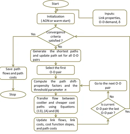
The flow logic of the SPSA is illustrated in Fig. 2. The algorithm starts with AON assignment or a warm start using previously known approximate solution as initialization. Next it checks for convergence criteria; if the initial solution does not satisfy the convergence criteria, then the SPSA

flow update logic is initiated. The SPSA equilibrates one O-D pair at a time in a sequential manner. The sequential approach helps to achieve faster convergence but it introduces the order bias in the solution. This issue has been tackled partially by updating path sets simultaneously for all the O-D pairs before commencing the flow shifts (move) for the O-D pairs. The shortest paths are generated for all the O-D pairs then those paths are included in the feasible path set which are not present in this set. Then the first O-D pair is brought into equilibration process. First, the path shift-propensity factors and threshold parameter (π) are computed and then flows are updated according to the move direction of the SPSA. The costs and slopes of the link cost functions, and then those of the paths, are updated after each move. Once an O-D pair is equilibrated using SPSA flow update logic, the next O-D pair in the sequence is brought into the equilibration process. Once all the O-D pairs are equilibrated, the convergence criterion is checked. If it is satisfied, the algorithm is terminated, else the next iteration is initiated. The convergence criterion adopted in this paper is the normalized gap (Ngap) of 10-6_{. The}

Ngap is defined as:

min

rs rs rs rs

k k k

r s k r s k

rs rs k k

r s k

c f

c f

c f

−

∑ ∑ ∑

∑ ∑ ∑

Start

Initialization ( AON or warm start)

Transfer flow between costlier and cheaper cost paths using Equations (13), (A) and (B)

Convergence criteria satisfied ?

Stop

Go to the next O-D pair Select the first

O-D pair

Is current O-D pair the last

O-D pair ? Yes No Yes

No

Update link flows, link costs, cost function slopes, and path costs Save path

flows and path costs

Generate the shortest paths and update path set for all O-D pairs

Compute the path shift-propensity factors and the threshold parameterπ

Inputs: Link properties, O-D demand, δ

Fig. 2.

The Implementation Flow Chart of SPSA Algorithm

In addition to the measure of convergence, two other aspects which are important from the implementation perspective are the step size λ and the proximity parameter

δ. The value of λ is obtained using the line search procedure that minimizes the value of objective function Z. For finding the λ, the line search technique needs a bound for it. It is obtained by satisfying the non-negativity constraints. As flows are added to the cheaper set of paths, the non-negativity constraints are not violated in the flow update process for them. For satisfying the non-negativity constraints in the flow update process for costlier set of paths, the following condition should be satisfied:

0

k k

f

− ∆ ≥

f

0

k k k

f

λρ

f

⇒

−

≥

(1

) 0

k k

f

λρ

⇒

−

≥

1 ,

k

k P

λ

ρ

⇒ ≤

∀ ∈

1

max( )

max

k

λ

ρ

⇒

=

1

0

max( )

k

λ

This implies that the minimum bound for the step size is zero, but its maximum bound depends on the path shift-propensity factor of the costliest path of the O-D pair and varies with O-D pairs, and from one iteration to the next. Hence, it is computed as the part of flow update process.

The proximity parameter δ decides the upper bound near the minimum cost of the O-D pair for selecting the cheaper paths set. In other words, δ sets the indifference band near minimum cost by specifying the

threshold limit πrsbetween the maximum cost path and minimum cost path. All paths that have cost less than πrs are assumed to be potentially attractive alternatives for drivers travelling on expensive paths (which has cost higher than πrs). The parameter

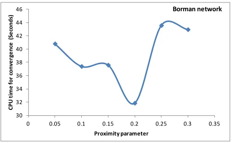
δ is the input to the algorithm and needs to be decided before using this algorithm. Based on sensitivity analyses for the two test networks, the value of 0.15 and 0.2 for this parameter was found to yield good results (Fig. 3 and Fig. 4) for the SPSA and has been adopted in this study.

8.7 8.75 8.8 8.85 8.9 8.95 9

0 0.05 0.1 0.15 0.2 0.25 0.3 0.35

CP

U

ti

m

e f

or

co

nv

er

gen

ce

(s

ec

on

ds

)

Proximity Parameter

Anaheim network

Fig. 3.

Calibration of Proximity Parameter for the Anaheim Network

30 32 34 36 38 40 42 44 46

0 0.05 0.1 0.15 0.2 0.25 0.3 0.35

CP

U

ti

m

e f

or

co

nv

er

gen

ce

(S

ec

on

ds

)

Proximity parameter

Borman network

Fig. 4.

5. Computational Experiments and

Results

Computational experiments are done to compare the convergence performance of the SPSA with respect to SMPA, F-W and social pressure algorithms. The computational experiments consider the two versions of SMPA. The first version (labeled SMPA) updates the path set and equilibrates the O-D pairs based on the sequential manner (for details see Kumar and Peeta, 2010). The second version (labeled SMPA-hybrid) was devised by Kumar and Peeta (2013) based on the insights from the experimental work done by Kumar et al. (2012) where O-D pairs are equilibrated based on the sequential approach but path sets are updated for all the O-D pairs simultaneously. The computational experiments use the Anaheim and Borman corridor networks as the test

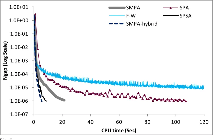
networks. The Anaheim network in southern California consists of 416 nodes, 914 links, and 1406 O-D pairs with non-zero demand. The Borman Corridor network in northwest Indiana consists of 197 nodes, 460 links and 1681 O-D pairs with non-zero demand. The computational environment used is a Dell precision workstation with Intel Xeon processors (2.67 GHz) and 64-bit Windows 7 operating system. The SPSA, SMPA, SMPA-hybrid, SPA and the F-W algorithm were coded in MATLAB and executed on the same computer. Some computationally intensive processes like updating flows, costs and cost functions derivatives for paths and links was performed by using the MEX (MATLAB executable) files coded in C. The computational performances of the algorithms are compared by plotting the

Ngap on the logarithmic scale versus the CPU time.

1.0E-07 1.0E-06 1.0E-05 1.0E-04 1.0E-03 1.0E-02 1.0E-01 1.0E+00 1.0E+01

0 20 40 60 80 100 120

N

gap

(L

og

S

cal

e)

CPU time (Sec)

SMPA SPA

F-W SPSA

SMPA-hybrid

Fig. 5.

The results of the computational experiment carried out for the Anaheim network are presented in Fig. 5. The performances of all the algorithms are similar in the initial stages but SMPA, SMPA-hybrid and SPSA perform better in the latter stages. The SMPA-hybrid and SPSA take about 9 seconds to reach the

Ngap of 10-6 _{(convergence level adopted here)}

followed by SMPA taking about 22 seconds, in contrast to social pressure algorithm which takes about 155 seconds to reach the same convergence level. The F-W algorithm lags behind throughout the latter stages and failed to reach convergence even after 200 seconds.

1.0E-07 1.0E-06 1.0E-05 1.0E-04 1.0E-03 1.0E-02 1.0E-01 1.0E+00 1.0E+01

0 50 100 150 200

N

gap

(L

og

S

cal

e)

CPU time (Sec)

SMPA SPA

F-W SPSA

SMPA-hybrid

Fig. 6.

Computational Results for the Borman Corridor Network

The results of the computational experiment for the Borman Corridor Network are presented in Fig. 6. The performance of the SPSA along with SMPA and SMPA-hybrid overtakes that of the SPA in the early stages and consistently improves until convergence. The SPSA takes less than one-third of the computational time compared to the SPA to reach convergence (Ngap of 10-6_{). In this case}

also F-W algorithm lags behind in later stages

Table 1

Sensitivity Analysis with Respect to Demand

De

m

an

d l

ev

el Convergence performance for Anaheim network

CPU time (seconds) for Convergence Number of iterations for convergence

SPA SMPA SMPA-_hybrid SPSA SPA SMPA SMPA-_hybrid SPSA

0.8 9.66 5.57 1.38 1.40 7 8 6 5

1 106.92 22.70 5.49 8.75 74 31 28 36 1.2 148.56 51.76 10.96 22.87 93 69 56 66

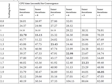
Table 2

Calibration of Optimal Parameters of SMPA for Anaheim Network

Sc

al

ing

fa

ct

or CPU time (seconds) for Convergence Inner

iterations = 9

Inner iterations = 8

Inner iterations = 7

Inner iterations = 6

Inner iterations = 5

Inner iterations = 1

0.8 26.01 26.97 27.86 32.01

0.9 24.37 24.96 27.27 28.52

1 24.38 26.50 26.18 29.22 30.31 76.91

1.1 22.70 23.13 25.32 26.30 29.06 70.29

1.2 43.77 51.22 24.02 25.41 26.94 67.69

1.3 43.06 47.75 23.43 24.46 25.85 61.37

1.4 41.78 46.96 47.74 23.99 24.38 60.51

1.5 39.37 47.33 47.91 22.98 23.67 54.74

1.6 37.00 47.05 43.17 56.80 23.93 54.69

1.7 46.02 43.56 41.92 52.40 23.23 49.48

1.8 34.29 45.49 40.90 51.53 23.29 48.98

1.9 33.79 30.47 36.89 35.82 44.05 46.05

2 32.12 29.66 35.16 37.05 42.17 47.03

2.1 40.19 50.54 57.33 104.15 88.64 82.00

The sensitivity analysis was done to find the performance of the algorithms with change in congestion level by varying the level of demand. The three levels of demand namely 0.8, 1.0 and 1.2 were tested for the Anaheim network. Here, demand level 1.0 correspond

convergence at different levels of demand. F-W algorithm is not included in this analysis because it failed to reach the convergence. The results of the sensitivity analysis show that the computational time (CPU time) as well as number of iterations required in reaching the convergence increases with the increase in congestion level for all the algorithms. In addition, the relative performances of the algorithms are similar to those observed in Fig. 5.

The superior performance of the SPSA compared to SPA and F-W algorithm can be attributed to the efficient utilization of the sensitivity of path costs relative to path flow in the form of slopes of the cost function in the flow update process and the transfer of flows to multiple potential paths simultaneously. The SPA is insensitive to the slope of cost function. In addition, in it the flow is shifted to just one path having the minimum cost though there may be many paths having cost equal to or close to the minimum cost path for that O-D pair. This leads to a substantial increase in the cost of the current minimum cost path as a result of flow update process. Thereby, in the next iteration, one of the paths with a cost equal or close to that of this path becomes the minimum cost path. This results in the oscillation of flows between the paths in the feasible set leading to an increase in the number of iterations to reach convergence. The comparatively similar convergence rates of the SPSA and the social pressure algorithms in the initial stages can be attributed to the computational cost of calculating the slopes of the cost functions in each iteration of the SPSA algorithm, though this is not particularly beneficial in the initial iterations due to the lesser number of efficient paths. In later stages, when more efficient paths are generated,

this burden is more than compensated by the gain in efficiency accrued by the optimal flow transfer to multiple potential paths.

calibration procedure. Hence, SPSA can act as potential alternative for SMPA-hybrid for practice.

6. Concluding Comments

This study proposes a new solution algorithm labeled as the SPSA for solving the static user equilibrium traffic assignment problem. The SPSA uses the concept of path shift-propensity factor inheriting insights from the social pressure algorithm. The use of the path shift-propensity factors concept provides a behaviorally consistent rationale for the flow update process relative to the network users seeking better routes in the real world. In addition, it uses the sensitivity of path cost with respect to path flow for deciding the proportion of network users switching to alternative attractive routes. Hence, the SPSA is likely to give more realistic path flow solutions given that multiple path flow solutions exist for the UETAP. In addition it is easy to implement in practice.

Based on the Gauss-Siedel decomposition technique, SPSA equilibrates one O-D pair at a time sequentially and operates in the space of path flows to achieve faster convergence. The sequential approach is likely to induce order bias in the solution space. In SPSA, this problem is tackled up to some extent by using the simultaneous path update technique. The flow update mechanism divides the set of feasible paths for an O-D pair into costlier and cheaper sets by calculating a threshold limit based on the maximum cost difference between the path costs (maximum path shift-propensity factors) and using the proximity parameter

δ. It uses the slopes of the cost function in the flow update process to determine the

move direction and shifts flow from the set of costlier paths to the set of cheaper paths between an O-D pair simultaneously. The step size for the move direction is obtained by a line search technique.

Computational experiments were performed for the Anaheim and Borman Corridor networks. They indicate that the SPSA along with SMPA-hybrid has a superior rate of convergence compared to the social pressure and F-W algorithms. The performance of the F-W algorithm lags behind in later stages and failed to reach convergence (Ngap of 10-6_).

All of the five algorithms exhibit a similar convergence rate in the initial stages, but SPSA, SMPA and SMPA-hybrid converges at a much faster rate in later stages and can be used for obtaining the UE solution for high convergence levels. SMPA-hybrid exhibited better convergence performance compared to SPSA. But SPSA represents the flow shift behavior more realistically in the flow update process and is easier to implement, and can act as a potential alternative for SMPA-hybrid in practice.

Acknowledgements

This study was partly funded by a project through the NEXTR A NS Center at Purdue University, USA. We would like to acknowledge valuable comments from researchers at NEXTRANS Center during the algorithm development and coding process.

References

Bar-Gera, H. 2010. Traffic assignment by paired alternative segments, Transportation Research Part B: Methodological. DOI: http://dx.doi.org/10.1016/j. trb.2009.11.004, 44(8-9): 1022-1046.

Bertsekas, D.P. 1976. On the Goldstein-Levitin-Poljak gradient projection method, IEEE Transactions on Automatic Control, 21(2): 174-184.

Bertsekas, D.P.; Gallager, R.G. 1987. Data Networks. Englewood Cliffs, Prentice-Hall, NJ, USA.

Bruynooghe, M.; Gilbert, A.; Sakarovitch, M. 1969. Une methode d’affectation du traffic. In Proceedings of the 4th International Symposium on the Theory of Road Traffic. Bundesminister fur Verkehr, Abt. Strassenbau, Bonn, Germany.

Beckmann, M.; McGuire, C.B.; Winsten, C.B. 1956.

Studies in the Economics of Transportation. Yale University Press, New Haven.

Dafermos, S. 1968. Traffic Assignment and Resource Allocation in Transportation Networks. PhD Dissertation, Johns Hopkins University, Baltimore, MD, USA.

Dafermos, S.; Sparrow, R. 1969. The traffic assignment problem for a general network, Journal of Research of the National Bureau of Standards, 73(B): 91-118.

Dial, R.B. 2006. A path-based user-equilibrium traffic assignment algorithm that obviates path storage and enumeration, Transportation Research Part B: Methodological. DOI: http://dx.doi.org/10.1016/j. trb.2006.02.008, 40(10): 917-936.

Dow, P.; Van Vliet, D. 1979. Capacity restrained road assignment, Traffic Engineering and Control, 20(6): 261-273.

Florian, M.; Nguyen, S. 1976. An application and validation of equilibrium trip assignment methods,

Transportation Science, 10(4): 374-390.

Florian, M.; Constantin, I.; Florian, D. 2009. A new look at the projected gradient method for equilibrium assignment, Transportation Research Record. DOI: http:// dx.doi.org/10.3141/2090-02, 2090: 10-16.

Florian, M.; Guelat, J.; Spiess, H. 1987. An efficient implementation of the “PARTAN” variant of the linear approximation method for the network equilibrium problem, Networks. DOI: http://dx.doi.org/10.1002/ net.3230170307, 17(3): 319-339.

Fukushima, M. 1984. A modified Frank-Wolfe algorithm for solving the traffic assignment problem,

Transportation Research Part B: Methodological. DOI: http://dx.doi.org/10.1016/0191-2615(84)90029-8, 18(2): 169-177.

Gallager, R.G. 1977. A minimum delay routing algorithm using distributed computation, IEEE Transactions on Communications. DOI: http://dx.doi.org/10.1109/ TCOM.1977.1093711, 25(1): 73-85.

Jaya k r ishnan, R .; Tsa i, W.K .; Prash ker, J.; Rajadhyaksha, S. 1994. A faster path-based algorithm for traffic assignment, Transportation Research Record, 1443: 75-83.

Knight, F.H. 1924. Some fallacies in the interpretation of social cost, Quarterly Journal of Economics. DOI: http:// dx.doi.org/10.2307/1884592, 38(4): 582-606.

Kumar, A.; Peeta, S. 2010. Slope-based multipath flow update algorithm for the static user equilibrium traffic assignment problem, Transportation Research Record. DOI: http://dx.doi.org/10.3141/2196-01, 2196(1): 1-10.

Kumar, A.; Peeta, S.; Nie, Y.M. 2012. Update strategies for restricted master problem for the user equilibrium traffic assignment problem: a computational study,

Transportation Research Record. DOI: http://dx.doi. org/10.3141/2283-14, 2283(1): 131-142.

Kupiszewska, D.; Van Vliet, D. 1998. Incremental traffic assignment: a perturbation approach. In Proceedings of the 3rd _{IMA International Conference on Mathematics in}

Transportation Planning and Control. 155-165.

Larsson, T.; Patriksson, M. 1992. Simplicial decomposition with disaggregate representation for the traffic assignment problem, Transportation Science. DOI: http://dx.doi.org/10.1287/trsc.26.1.4, 26(1): 4-17.

LeBlanc, L.J. 1973. Mathematical Programming Algorithms for Large Scale Network Equilibrium and Network Design Problems. PhD Dissertation, Department of Industrial Engineering and Management Science, Northwestern University, USA.

LeBlanc, L.J.; Helgason, R.V.; Boyce, D.E. 1985. Improved efficiency of the Frank-Wolfe algorithm for convex network problems, Transportation Science. DOI: http://dx.doi.org/10.1287/trsc.19.4.445, 19(4): 445-462.

LeBlanc, L.J.; Morlok, E.K.; Pierskalla, W.P. 1975. An efficient approach to solving the road network equilibrium traffic assignment problem, Transportation Research. DOI: http://dx.doi.org/10.1016/0041-1647(75)90030-1, 9(5): 309-318.

Lee, D.H.; Nie, Y.M. 2001. Accelerating strategies and computational studies of the Frank-Wolfe algorithm for the traffic assignment problem, Transportation Research Record. DOI: http://dx.doi.org/10.3141/1771-13, 1771: 97-105.

Lu, S.; Nie, Y.M. 2010. Stability of user-equilibrium route flow solutions for the traffic assignment problem,

Transportation Research Part B: Methodological. DOI: http:// dx.doi.org/10.1016/j.trb.2009.09.003, 44(4): 609-617.

Luenberger, D.G. 1973. Introduction to Linear and Nonlinear Programming. Addison-Wesley, Reading, Massachusetts.

Meyer, G. 1974. Accelerated Frank-Wolfe algorithms,

SI A M Journal on Control. DOI: http://d x.doi. org/10.1137/0312050, 12(4): 655-663.

Nguyen, S. 1974. An algorithm for the traffic assignment problem, Transportation Science. DOI: http://dx.doi. org/10.1002/net.3230100303, 8(3): 203-216.

Rosen, B. 1960. The gradient projection method for nonlinear programming, part I linear constraints,

Journal of the Society for Industrial and Applied Mathematics, 8(1):181-217.

Rossi, T.F.; McNeil, S.; Hendrickson, C. 1989. Entropy model for consistent impact-fee assessment, Journal of Urban Planning and Development, ASCE. DOI: http:// dx.doi.org/10.1061/(ASCE)0733-9488(1989)115:2(51), 115(2): 51-63.

Sheffi, Y. 1985. Urban Transportation Networks: Equilibrium Analysis with Mathematical Programming Methods. Prentice-Hall, Inc., Englewood Cliffs, New Jersey.

Wardrop, J. 1952. Some theoretical aspects of road traffic research. In Proceedings of the Institution of Civil Engineers, 2: 325-378.

Weintraub, A; Ortiz, C.; Gonzales, J. 1985. Accelerating convergence of the Frank-Wolfe algorithm, Transportation Research Part B: Methodological. DOI: http://dx.doi. org/10.1016/0191-2615(85)90018-9, 19(2): 113-122.