A pathway to eliminate the gas flow dependency of a hydrocarbon sensor for automotive exhaust applications

https://doi.org/10.5194/jsss-7-79-2018

© Author(s) 2018. This work is distributed under the Creative Commons Attribution 4.0 License.

A pathway to eliminate the gas flow dependency of a

hydrocarbon sensor for automotive exhaust applications

Gunter Hagen, Antonia Harsch, and Ralf Moos

Bayreuth Engine Research Center (BERC), Department of Functional Materials, University of Bayreuth, 95440 Bayreuth, Germany

Correspondence:Gunter Hagen (gunter.hagen@uni-bayreuth.de)

Received: 18 October 2017 – Revised: 11 January 2018 – Accepted: 14 January 2018 – Published: 16 February 2018

Abstract. Gas sensors will play an essential role in future combustion-based mobility to effectively reduce emissions and monitor the exhausts reliably. In particular, an application in automotive exhausts is challenging due to the high gas temperatures that come along with highly dynamic flow rates. Recently, a thermoelectric hy-drocarbon sensor was developed by using materials which are well known in the exhausts and therefore provide the required stability. As a sensing mechanism, the temperature difference that is generated between a catalyt-ically activated area during the exothermic oxidation of said hydrocarbons and an inert area of the sensor is measured by a special screen-printed thermopile structure. As a matter of principle, this thermovoltage signifi-cantly depends on the mass flow rate of the exhausts under certain conditions. The present contribution helps to understand this cross effect and proposes a possible setup for its avoidance. By installing the sensor in the correct position of a bypass solution, the gas flow around the sensor is almost free of turbulence. Now, the signal depends only on the hydrocarbon concentration and not on the gas flow. Such a setup may open up new possibilities of applying novel sensors in automotive exhausts for on-board-measurement (OBM) purposes.

1 Introduction

Automotive exhausts are particularly challenging for gas sen-sors (Deutschmann and Grunwaldt, 2013; Twigg, 2003). On the one hand, fast and detailed information about the actual (mostly low) concentration of a certain gas component is nec-essary for efficient after-treatment technologies. On the other hand, high temperatures, high dynamically changing flow characteristics and undefined poisoning components (such as oil, ashes, soot or harmful gases) affect the sensor response negatively (Riegel et al., 2002; Ojha et al., 2017b). In the past decades, only a handful of materials were successfully ap-plied in exhaust gas sensing devices. Mostly, zirconia-based sensors are applied because of their thermal and mechani-cal robustness in combination with their functional proper-ties. Applications are lambda or NOxsensors, but zirconia is also used as a platform material for soot sensors (Ochs et al., 2010).

Ongoing legislation and minimization of emission limits require more complex after-treatment systems, and therefore, novel exhaust gas sensors are needed which are sensitive to

special gas components (Moos, 2006, 2009). For example, diesel oxidation catalysts (DOCs) should include an NO2or a hydrocarbon (HC) sensor to ensure stable and accurate on-board diagnosis (OBD). Novel sensors also could play an important role for on-board measurements (OBMs) as a fu-ture vision beyond OBD. The introduction of real-driving-emissions testing (RDE) is the first step towards a permanent exhaust gas analysis during operation.

operation, and finally it validates the simulation using mea-surements.

2 Principle of a thermoelectric hydrocarbon sensor

In the following section, the principle of a thermoelectric gas sensor is explained. Such devices are used in this study for two reasons: firstly, thermoelectric sensors are promis-ing candidates for application in harsh conditions. Setup and manufacturing are simple (which also means they are inex-pensive for serial production) and can be realized completely using high-temperature stable materials, which ensures long-term stability. We have already demonstrated the feasibility of HC detection for OBD purposes in diesel exhausts by this principle. Secondly, such sensors give a direct response on temperature gradients on the device originating from outer impacts like the gas flow inhomogeneity. Therefore, the ther-moelectric sensors are ideal candidates for this investigation, presuming that the evaluated effects also appear with any other kind of gas sensor (Ritter et al., 2017).

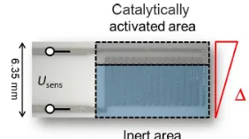
The thermoelectric sensor used here as depicted in Fig. 1 compares two areas of the device: one area is catalytically activated by a porous Pt-loaded alumina thick film; the other area is inert. Reducing gases react on the Pt catalyst; there-fore a temperature gradient1T between both areas is formed due to exothermic heat on the catalyst-coated side. This tem-perature gradient is measured by a thermopile structure fully manufactured in thick-film technology. The thermovoltage Usens resulting from the Seebeck coefficients of the partic-ipating materials yields a linear response to the reducing gas concentration. The sensor characteristics can be improved by using substrate materials with lower thermal conductivity or by increasing the number of thermopiles in the sensing struc-ture. As thermopile materials, commercially available thick-film pastes are appropriate such as Au and Pt. To improve the high-temperature stability, we also successfully applied Pt/PtRh (type S) thermocouples (Kita et al., 2015). The ab-solute sensor temperatureTabs(e.g., 600◦C) is adjusted by an internal thick-film heater on the reverse side of the sensor. It keeps the catalyst active. For more details, see Wiegärtner et al. (2015), Ritter et al. (2017), Hagen et al. (2017) and Ojha et al. (2017a).

Figure 1.Sensor setup: screen-printed thermopiles (Pt/PtRh on alumina substrate) allow a thermovoltageUsensto be measured be-tween the inert and the catalytically activated area of the sensor. This voltage is a function of exothermicity. A heater on the reverse side adjusts the absolute sensor temperature.

3 Preliminary theoretical considerations

Ideally, the sensor signal Usens is only dependent on the exothermic heat that is caused by the oxidation of the test gas at the catalytically activated area. Without test gas, the temperature gradient and therefore the voltage signal should be zero. In fact, in that case, one measures an offset voltage, stemming from slight nonuniformities of the screen-printed heater tracks or asymmetric heat conduction to the ambiance, which could be, e.g., affected by the sensor mounting. For a constant operation temperature (e.g.,Tabs=600◦C) in a sta-ble atmosphere, this offset should not change and can be sub-tracted before the first measurement.

The most challenging issue is probably the cooling ef-fect of flowing gas reaching the sensor surface. Any case of asymmetric cooling, e.g., from turbulence around the device, causes, as a matter of principle, strong influences on the mea-sured voltageUsens. Former investigations showed that an ap-plication of the sensor in the full flow of automotive exhausts leads to strong voltage changes according to changing engine operation conditions and variable flow rates and gas temper-atures. Here, it is almost impossible to separate the HC effect from these voltage changes and to evaluate the actual gas concentration with the required low uncertainty.

In order to counteract these drawbacks, the gas should flow symmetrically on both sides of the functional sensor element, which should be mounted perpendicular to the gas flow. This should lead to uniform cooling effects on both sides, and hence, should cause no temperature gradient between the catalytically coated area and the inert area. The gas flow it-self should be laminar with no turbulence. To visualize these influences, both cases were FEM (finite element method)-simulated with the help of COMSOL Multiphysics®.

Figure 2.Simulated flow lines around a sensor element (cross section in top view) for a 90◦orientation(a)and a slightly rotated case(b). Coloring indicates the temperature distribution (simulation parameters are as follows: gas flow 1 L min−1, gas temperature 20◦C, sensor heating 1.27 W).

indicates its temperature distribution, also changes symmet-rically. No gradient between the two areas on the sensor’s surface is visible. For the rotated substrate, however, asym-metric cooling due to the differing flow characteristics oc-curs and is clearly obvious in Fig. 2b. This would lead to a flow-dependent temperature gradient that would significantly affect the sensor signal.

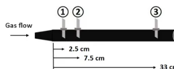
In the model described, a laminar flow profile was as-sumed. Now, in a second simulation, the influence of turbu-lence around the sensor should be examined. Therefore, we chose a geometry close to the real setup. The gas supply is connected to a cone-shaped gas inlet that widens the cross section to the width of the sensor chamber (100=2.54 cm). We prove the flow lines for three different sensor mounting positions, characterized by their distance to the cone: (1) near to the cone end (2.5 cm), (2) at a little more distance from the inlet (7.5 cm) and (3) at a large distance from the cone (33 cm). In this model, the sensors are mounted at a 90◦ po-sition, directly facing the gas flow (Fig. 3).

Now, the flow lines are visualized for positions (1) and (3). A significant difference concerning the flow character occurs. Figure 4 shows the result for the cross-sectional side view through the sensor middle axis. In the cone region when the profile widens up, a dead space is visible with back streaming gas (loops in the simulated flow lines). The flow has not been fully established yet. If one evaluates the gas ve-locitywin flow direction over the cross section (position and diameter indicated by the green line) and plots these data in relation to the maximum velocitywmaxfor a fully established flow (i.e., for an ideal parabolic flow profile) over the radial distance−1.25 cm <r<+1.25 cm, it becomes clear that neg-ative values also occur (back ward flow), and a high peak value indicates huge differences of the gas velocity over the chamber radius (Fig. 4a).

Mounting position (1) therefore causes much turbulence behind the sensor; therefore the sensor measurement at this position will be strongly affected be the gas flow rate

Figure 3.Scheme of the sensor tube used for modeling as well as for experiments with three different sensor mounting positions depending on the distance from the cone end. The inner diameter of the chamber is 2.54 cm (100).

(Fig. 4b). In contrast to that, a laminar flow (with a parabolic shape in Fig. 4a) is much less disturbed by the sensor when mounted in position (3). The flow lines are more smooth be-hind the sensor (Fig. 4c), and the laminar profile is restored much earlier than in case (1).

Concluding these results, a flow-independent measure-ment should only be possible if the precondition of ideal per-pendicular mounting and a laminar flow profile facing the sensor are fulfilled. This shall now be verified by experi-ments.

4 Experimental results and discussion

(Wiegärt-Figure 4.Cross-sectional side view of simulated gas flow lines in the setup described (Fig. 3) for 90◦sensor mounting at position (1) and position (3)(b, c)and evaluated gas velocity over the inner diameter 2.5 cm in front of the sensor (green line) for both cases(a).

ner et al., 2015). Data were obtained using a Keithley DMM 2700.

4.1 Measurements in air

From the FEM modeling it was concluded that a laminar flow that impacts the sensor surface directly and perpendicularly should be a necessary precondition for flow independency. We proved this assumption in experiments. Sensor chamber and sensor geometry data are similar to the modeling param-eters (see Fig. 3). For each mounting position, we varied the gas flow V˙ from 0 to 35 L min−1 and measured the sensor response for a certain time (about 1 min). The sensors were operated constantly at 300◦C as absolute sensor tempera-ture. Readjusting for different flow rates is done by control-ling the four-wire resistance in the heater structure to a con-stant value (Bischof et al., 1999; Wiegärtner et al., 2015). For data visualization, the temperature gradient (1T, concerning the sensor’s front side) was calculated from the voltage sig-nal and plotted over the gas flow rate. Therefore, a couple of values for each flow rate (we measured about 30 values during 1 min of constant flow) indicate by their scattering whether the signal is noisy for that flow rate and, to that ef-fect, whether turbulence occurs. As expected, we found sig-nificant differences between the three different mounting po-sitions mentioned above (Fig. 5): position (1) leads to high scattering within each flow rate (range=2 K, i.e.,±1 K) and even the mean values (calculated within each flow rate) differ strongly between the different flow rates (from1T=4 K @ 2 L min−1to∼1 K @ 15 L min−1and 1.5 K @ 35 L min−1). Better results can be achieved for mounting position (2). Here, the mean value is mostly constant (1T=2 K) for all flow rates, but scattering is still high. Measurements at posi-tion (3) show the best results, where a constant mean value of1T=1.5 K between 5 and 35 L min−1with stable values (scattering±0.25 K) occurs.

At position (3), we also did additional tests concerning the mounting orientation of the sensor. Here, the expectation was also met: changing the mounting angle by +5◦ leads to a higher mean value. Interestingly, this mean value is mostly

Figure 5.Measured sensor signal (Tabs=300◦C) with dependence on the gas flow rate (temperature difference1T between both sen-sor areas calculated from the measured thermovoltage) for the three different mounting positions described, (1), (2) and (3),(a–c)and for a slightly rotated mounting at position (3)(d).

Figure 7.Sensor raw signal for stepwise HC admixture (750 ppm) in different flow conditions: variable flow rate (2, 3, and 4 L min−1) at position (1)(a)and at position (3)(b).

constant. A change by −10◦decreases the mean value, and furthermore, due to the higher discrepancy from the ideal case (see Fig. 2), a significant flow dependency occurs. Scat-tering is not affected by the mounting orientation, so it seems that this is an effect of turbulence, considering its dependency from the mounting position.

In real-world applications, the sensor has to provide cor-rect results, even under highly dynamic flow rate changes. Therefore, in the next experiment it should be proven whether the positive result can be reproduced in unsteady flow conditions. Again, compressed air was used as the test gas. The sensor was mounted at a 90◦ angle at position (3) and operated at Tabs=300◦C. The flow rate was changed rapidly in the range between 0 and 48 L min−1as indicated in Fig. 6. As a result, the sensor voltage even now scattered only in a small range around a stable mean value (1T =1.5 K, as already seen in Fig. 5c) during the whole test.

4.2 HC concentrations’ measurements

In the next step, the flow variation was combined with a step-wise hydrocarbon admixture to demonstrate the performance of the system presented. The sensors were mounted at posi-tions (1) and (3) in the tube described for comparison. The flow rate was varied from 2 to 4 L min−1; the base gas con-tained 10 % O2 in N2. For the test gas we added 750 ppm propene to each measurement. For better understanding, the results are shown as raw data (voltage signalUsens) over time (Fig. 7).

When regarding the results at mounting position (1), the typical issues described above are visible. The offset value as well as scattering strongly depends on even small changes in the flow rate. In each run, the HC step leads to a sensor response that is not even detectable anymore for the high-est flow rates. Due to the offset changes, one cannot distin-guish between both effects as long as the flow rate is un-known. For mounting position (3), the flow dependency is highly reduced. Both offset changes and scattering are mostly avoided. Here, the sensor response is a direct measure of the HC content in the test gas, independent of the gas flow rate.

This setup provides an opportunity for stable and repeat-able HC measurements. Therefore, we suggest arranging gas

sensors that are prone to dynamic gas flow changes to be in-stalled in such a way that no turbulence occurs around the sensor.

5 Conclusion

The flow dependency, as the main problem of robust thermo-electric gas sensors, can be avoided by mounting the sensor in an appropriate sensor tube. Here, the gas flow character-istics are defined in such a way that the gas flow around the sensor is mostly laminar. Cooling effects arising from the gas flow are symmetric, and therefore, the sensor signal is not af-fected by the flow rate anymore. With these findings, one of the major drawbacks of chemical gas sensors to be applied in automotive exhausts could be resolved. Now, on-board-measurement systems using chemical gas sensors come into question because several novel sensor principles might profit from such a bypass solution. In a first step of further work, we will aim to reproduce such results in real exhausts.

Data availability. All relevant data are given in the article. Most of the data are raw data as shown in the diagrams and explained in the text.

Competing interests. The authors declare that they have no con-flict of interest.

Special issue statement. This article is part of the special issue “Sensor/IRS2 2017”. It is a result of the AMA Conferences, Nurem-berg, Germany, 30 May–1 June 2017.

Acknowledgements. The authors thank Sven Wiegärtner, who manufactured the sensors.

https://doi.org/10.1002/cite.201200188, 2013.

Hagen, G., Leupold, N., Wiegärtner, S., and Moos, R.: Sensor Tool for Fast Catalyst Material Characterization, Top. Catal., 60, 312– 317, https://doi.org/10.1007/s11244-016-0617-8, 2017. Kita, J., Wiegärtner, S., Moos, R., Weigand, P., Pliscott, A.,

LaBranche, M. H., and Glicksman, H. D.: Screen-printable type S thermocouple for thick-film technology, Procedia Engineer., 120, 828–831, https://doi.org/10.1016/j.proeng.2015.08.692, 2015.

Moos, R.: Automotive Exhaust Gas Sensors, in: Encyclopedia of Sensors, edited by: Grimes, C. A., Dickey, E. C., and Pishko, M. V., 1, 295–312, American Scientific Publishers, Stevenson Ranch, USA, 2006.

Moos, R.: Recent Developments in Automotive Exhaust Gas Sensing, Proceedings SENSOR 2009, I, 227–231, https://doi.org/10.5162/sensor09/v1/b5.1, 2009.

Moos, R., Sahner, K., Fleischer, M., Guth, U., Barsan, N., and Weimar, U.: Solid State Gas Sensor Research in Germany: a Status Report, Sensors, 9, 4323–4365, https://doi.org/10.3390/s90604323, 2009.

Ochs, T., Schittenhelm, H., Genssle, A., and Kamp, B., Particu-late Matter Sensor for On Board Diagnostics (OBD) of Diesel Particulate Filters (DPF), SAE Int. J. Fuels Lubr., 3, 61–69, https://doi.org/10.4271/2010-01-0307, 2010.

2017b.

Riegel, J., Neumann, H., and Wiedenmann, H.-M., Exhaust gas sen-sors for automotive emission control, Solid State Ionics, 152– 153, 783–800, https://doi.org/10.1016/S0167-2738(02)00329-6, 2002.

Ritter, T., Wiegärtner, S., Hagen, G., and Moos, R.: Simula-tion of a thermoelectric gas sensor that determines hydro-carbon concentrations in exhausts and the light-off tempera-ture of catalyst materials, J. Sens. Sens. Syst., 6, 395–405, https://doi.org/10.5194/jsss-6-395-2017, 2017.

Twigg, M. V.: Automotive Exhaust Emissions Control, Platin. Met. Rev., 47, 157–162, 2003.