R E S E A R C H
Open Access
Alternative approaches for econometric
modeling of panel data using mixture
distributions
Judex Hyppolite
Correspondence: [email protected] Department of Economics, Finance, and Real Estate, Monmouth University, 400 Cedar Avenue, 07776, West Long Branch, New Jersey, USA
Abstract
The economic researcher is sometimes confronted with panel datasets that come from a population made of a finite number of subpopulations. Within each subpopulation the individuals may also be heterogenous according to some unobserved
characteristics. A good understanding of the behavior of the observed individuals may then require the ability to identify the groups to which they belong and to study their behavior across groups and within groups. This may not be a complicated exercise when a group indicator variable is available in the dataset. However, such a variable may not be included in the dataset; and as a result, the econometrician is forced to work with the marginal distribution of the observed response variable, which takes the form of a mixture distribution.
One can model a given response variable with a variety of mixture distributions. In this paper, I present several related mixture models. The most flexible one is an extension of the model by Kim et al. (2008) to the panel data setting.
I have reviewed the estimation of some of these models by the
Expectation-Maximization (EM) algorithm. The intent is to exploit the nice convergence properties of this algorithm when it is difficult to find good starting values for a
Newton-type algorithm. I have also discussed how to compare these models and ultimately identify the one that provides the best fit to the data set under investigation. As an application I examine the investment behavior of U.S. manufacturing firms.
Keywords: Panel data, Mixture of distributions, Hidden Markov models, Heterogeneity
Introduction
To model the heterogeneity of economic agents I present a series of panel data mix-ture models of increasing degree of flexibility and complexity and show how they can be used to handle at least two types of heterogeneity: heterogeneity with respect to group membership, and heterogeneity with respect to within group differences in individual characteristics. I have also reviewed the methods of estimation of some of these models via the Expectation-Maximization algorithm. The objective is to take advantage of the nice convergence properties of this algorithm when it is difficult to find good starting val-ues for a newton-type algorithm. I have also reviewed some statistical tests that can be used to choose the best models among those discussed in this paper.
Heterogeneity is an important problem faced by the statistician or the econometri-cian trying to infer the behavior of economic agents from available data sets. Economic decison makers are heterogeneous in their characteristics and they usually operate in heterogeneous (different) environments. As a result, their behavior generate data whose distributions are sometimes difficult to approximate with the traditional single com-ponent econometric models. To deal with this problem, often economists divide their sample into groups using observed variables such as time (in time series) or other indi-vidual characteristics (in time series and longitudinal data). The groups obtained this way are usually static and may differ from alternative groups obtained using different observed variables.
While this strategy may allow the researchers to draw some useful conclusions, it is less attractive than the approach that uses multiple characteristics for determining group membership. It is also less flexible than the approach that allows for the possibility that an individual changes group membership depending on the evolution of his characteristics and of the conditions that he is facing. Lastly, it is much less flexible than the approach that offers a unified way (one step method) to make inference about both group mem-bership and behavior. Mixture of distribution models offer such flexibility. These models are justified not only in theory, because they offer a nice way to model heterogeneity, but also in practice since they can be used to provide a semi-parametric approxima-tion to the non-standard distribuapproxima-tions of some economic variables at a reasonable cost (McLachlan and Peel 2000). Mixture of distributions are in fact at the crossroad between parametric and non parametric families of distributions. They are parametric because each component distribution usually belongs to a parametric family of distributions, and they are non-parametric because it is possible to provide a very good approximation to the distribution of some variables by increasing the number of components of the mixture (Fink 2007).
The models
Several alternative mixture distributions can be used to model the bivariate process con-stituted by an economic agent’s decision and its group membership. In the following sections, nine such models are described going from the simplest to the most compli-cated. All of the models are assumed to be made of two components, but extension to more than two components is not difficult.
The models can be used to study several different economic phenomena such as households consumption under financial constraints, firms investment under financial constraints, households demand for money, household use of healthcare, etc. In what fol-lows I will use the example of investment choices under financial constraints to motivate the specifications.
A finite mixture model with constant mixing proportions (M1)
Consider the vector of random variables(Yit,Wit)whereYitrepresents agenti’s decision
at timet(;t=1,. . .,Ti;i=1,. . .n) whileWitis a discrete random variable
wit=
1 if agentibelongs to group 1 at timet 2 otherwise
In a model about firms’ investment decisions under financing constraints,Yitwould
rep-resent firmi’s investment rate at timet, whileWitwould be the firm’s financial status at
that time.YitandWitare assumed to be dependent in the sense that the agent’s decision
depends on the group he belongs to; more precisely I assume that
fyit|wit=1;β1,σ1
=φyit;xitβ1,σ1
fyit|wit=2;β2,σ2
=φyit;xitβ2,σ2
, σ1>0,σ2>0,
whereφ(.)is the density function of a univariate normal distribution andxitis a row
vec-tor of covariates including individual characteristics that influence the agent’s decisions, andβ1andβ2are column vectors of parameters. The joint density of(yit,wit)is given by
fyit,wit;βv,σv
=p(wit=v)φ
yit;xitβv,σv
,v=1, 2,
and the marginal density ofyitis
fyit;β1,σ1,β2,σ2=p(wit=1)φyit;xitβ1,σ1+p(wit=2)φyit;xitβ2,σ2.
Let
θ =π,β1,σ1,β2,σ2
.
When Wit follows a Bernoulli distribution with parameter, π, the marginal density
becomes
f(yit;θ)=πφ
yit;xitβ1,σ1
+(1−π)φyit;xitβ2,σ2
.
Parameters Estimation
The parameters of the preceding model can be estimated using maximum likelihood. The complete-data likelihood is
Lc(θ)= n
i=1
Ti
t=1
πφyit;xitβ1,σ1
I(wit=1)(
1−π)φyit;xitβ2,σ2
1−I(wit=1)
,
while the marginal likelihood is
L(θ)= n
i=1
Ti
t=1
πφyit;xitβ1,σ1
+(1−π)φyit;xitβ2,σ2
.
Since Wit is missing, maximizing the marginal likelihood appears to be the most
natural estimation approach. However, the Expectation-Maximization (EM) algorithm (Dempster et al. 1977) offers a much simpler alternative. This algorithm maximizes the complete-data likelihood after augmenting the data for the missing variableWitduring
the expectation step.
The two main steps of the algorithm are the following:
• E-Step (Expectation Step)
During this step, an intermediate quantity
Qθ,θ=Ewit
logLc(θ)|θ
• M-setp (Maximization step)
during which the following maximization problem is solved
ˆ
θ =argmax
θ Q
θ,θ
Subject to:
Various appropriate constraints.
For the model considered here
Qθ,θ=Ewit
logLc(θ)|θ
=
n
i=1
Ti
t=1
1−Ewit
I(wit=1)|yit;θ ln(1−π)+lnφ
yit;xitβ2,σ2
+
n
i=1
Ti
t=1
Ewit
I(wit=1)|yit;θ lnπ+lnφ
yit;xitβ1,σ1
.
Defining
Ewit
I(wit=1)|yit;θ
yit=y(it1) (1)
1−Ewit
I(wit=1)|yit;θ
yit=y(it2) (2)
Ewit
I(wit=1)|yit;θ
xit=x(it1) (3)
1−Ewit
I(wit=1)|yit;θ
and,
y(111),. . .,y(11T1),. . .,y(nT1)n =y(1) (5)
y11(2),. . .,y(12T1),. . .,y(nT2) n
=y(2) (6)
w11(1),. . .,w(11T1),. . .,w(nT1) n
=w(1) (7)
w11(2),. . .,w(12T1),. . .,w(nT2) n
=w(2) (8)
x(111),. . .,x(11T1),. . .,x(nT1)n =x(1), (9)
x(112),. . .,x(12T1),. . .,x(nT2)n =x(2) (10)
the expected complete-data log-likelihood can be written as
Qθ,θ=
n i=1 Ti t=1
1−Ewit
I(wit=1)|yit;θ
ln(1−π)
+ n i=1 Ti t=1 Ewit
I(wit=1)|yit;θ
lnπ
− lnσ22 2 n i=1 Ti t=1
1−Ewit
I(wit=1)|yit;θ
− lnσ12 2 n i=1 Ti t=1 Ewit
I(wit=1)|yit;θ
− 1
2σ22
y(2)−x(2)β2
y(2)−x(2)β2
− 1
2σ12
y(1)−x(1)β1
y(1)−x(1)β1 .
After solving the system of equations derived from the first order conditions we get
ˆ
π=
n i=1
Ti t=1Ewit
I(wit=1)|yit;θ
n
i=1Ti
ˆ
β1=
x(1) x(1)
−1
x(1) y(1)
ˆ
β2=
x(2) x(2)
−1
x(2) y(2)
ˆ
σ2 1 =
y(1)−x(1)βˆ1
y(1)−x(1)βˆ1
n i=1
Ti
t=1Ewit(I(wit=1)|yit;θ)
ˆ
σ2 2 =
y(2)−x(2)βˆ2
y(2)−x(2)βˆ2
n i=1
Ti t=1
1−Ewit(I(wit=1)|yit;θ)
Once we get an estimate forEwit(I(wit=1)|yit;θ), computing the preceding estimators
is simple. In fact,
Ewit
I(wit=1)|yit;θ
=probwit =1|yit;θ
= prob(wit=1)×f
yit|wit=1;θ fyit;θ
= πφ
yit;xitβ1,σ1
πφyit;xitβ1,σ1
+(1−π)φyit;xitβ2,σ2 .
So, if we knowπ,β2,σ2
andβ1,σ1
we can find an estimate forEwit|yit;θ
. The EM algorithm for this model can be summarized as follows:
1. Choose initial valuesθ0=π0,β01,σ10,β02,σ20
2. ComputeEwit|yit;θ0
for each observation 3. SubstituteEwit|yit;θ0
in the complete-data log-likelihood
4. Find new values for the parametersθ1=π1,β11,σ11,β12,σ21by maximizing the complete-data likelihood
5. Compute error= |L
θ1−Lθ0| |Lθ0|
6. If error is higher than a chosen tolerance level, repeat step 2 with the last estimates for the parameters
7. Otherwise, stop; the last estimates are the maximum likelihood estimates.
This algorithm is attractive not only because it provides an intuitive interpretation of the estimation, but also because of its monotone and global convergence properties. It has been proved (McLachlan and Krishman 1997) that the log-likelihood is non-decreasing at each consecutive iteration. This property is very useful for detecting programming errors. Moreover, the global convergence property allows for more flexibility in the choice of starting values than is possible with a Newton-type algorithm.
However, the EM Algorithm is criticized not only because it converges at a low rate, but also because it does not supply automatically an estimate of the covariance matrix of the parameters (McLachlan and Krishman 1997). The Hessian necessary to obtain an estimate of the information matrix in the maximum likelihood setting is not used in the computations. There have been several solutions proposed in the literature to solve this problem. The most notable one is provided by Louis (1982).
Note that according to this model the probability that an economic agent belongs to a certain group remains the same every period. In a dynamic economic environment this assumption is too restrictive. For example, the financial status of a firm cannot be deter-mined by flipping a coin; it is more likely to be dependent on the firm’s performance, its characteristics and on the economic conditions it is facing. Thus, several observed vari-ables should help in determining group membership. So, a more realistic model should allow for covariates dependent mixing proportions.
A finite mixture model with smoothly varying mixing proportions (M2) Suppose
wit=
where
w∗it=zitγ −it,it ∼N(0, 1) (11)
zitis a row vector of covariates that impact the probability for an agentito belong to a certain group andγ is a column vector of parameters.
The group membership equation (Eq. 11) could be modeled with the logistic distribu-tion. Since I want to compare all the models, I would also need to model endogeneity in the same setting and this is not straightforward. It is then better to use the normal dis-tribution and take advantage of the nice properties of the conditional disdis-tributions of a partitioned normal random vector. Let
θ =γ,β1,σ1,β2,σ2
.
The joint density of(Yit,Wit)is
f(yit,wit;θ)=
p(wit=1)φ(yit;xitβ1,σ1)
p(wit=2)φ(yit;xitβ2,σ2)
=
p(it<zitγ)φ(yit;xitβ1,σ1)
p(it≥zitγ)φ(yit;xitβ2,σ2)
=
(zitγ)φ(yit;xitβ1,σ1) (1−(zitγ)) φ(yit;xitβ2,σ2)
,
and the marginal density is
f(yit;θ)=(zitγ)φ(yit;xitβ1,σ1)+(1−(zitγ)) φ(yit;xitβ2,σ2),
where (.) is the univariate cumulative distribution function of a standard normal random variable.
Parameters Estimation
This model can also be estimated using the EM algorithm. The complete-data likelihood is
Lc(θ)= n
i=1
Ti
t=1
(zitγ)φ(yit;xitβ1,σ1)
I(wit=1)(
1−(zitγ)) φ(yit;xitβ2,σ2)
1−I(wit=1)
and the marginal likelihood
L(θ)= n
i=1
Ti
t=1
(zitγ)φ
yit;xitβ1,σ1
+(1−(zitγ)) φ
yit;xitβ2,σ2
.
The intermediate EM quantity is
Q(θ,θ)=Ewit(log(L
c(θ)|θ))
=
n
i=1
Ti
t=1
1−Ewit(I(wit=1)|yit;θ) ln(1−(zitγ)+lnφ(yit;xitβ2,σ2)
+
n
i=1
Ti
t=1
Ewit(I(wit=1)|yit;θ
)ln(zitγ)+lnφ(y
it;xitβ1,σ1)
Using Eqs. (1) - (10), the intermediate EM quantity can be rewritten as
Q(θ,θ)=
n
i=1
Ti
t=1
1−Ewit
I(wit=1)|yit;θ
ln(1−(zitγ)
+
n
i=1
Ti
t=1
Ewit
I(wit=1)|yit;θ
ln(zitγ)
−lnσ22 2
n
i=1
Ti
t=1
1−Ewit
I(wit=1)|yit;θ
−lnσ12 2
n
i=1
Ti
t=1
Ewit
I(wit =1)|yit;θ
− 1
2σ22
y(2)−x(2)β2
y(2)−x(2)β2
− 1
2σ12
y(1)−x(1)β1
y(1)−x(1)β1 .
The first order conditions for the maximization ofQ(θ,θ) will not produce a closed form solution forγ, but the estimators forβ1,σ1,β2,σ2are the same as before. The intermediate EM quantity being separable in the different group of parameters,γˆ can be obtained separately using the Newton-type method:
ˆ
γ =argmax γ
⎛ ⎝n
i=1
Ti
t=1
1−Ewit
I(wit=1)|yit;θ
ln(1−(zitγ)
+
n
i=1
Ti
t=1
Ewit
I(wit=1)|yit;θ
ln(zitγ)
⎞ ⎠
Also
Ewit
I(wit=1)|yit;θ
= (zitγ)φ(yit;xitβ1,σ1)
(zitγ)φyit;xitβ1,σ1
+(1−(zitγ))φyit;xitβ2,σ2
The EM algorithm can be implemented exactly as before.
An Endogenous Switching Regression Model (M3)
mixture models they are defined only on the corresponding sub-populations (Maddala 1999). The model can be presented as follows:
wit=
1 ifw∗it >0 2 otherwise
w∗it=zitγ −it
yit=
yit1=xitβ1+u1it, ifwit=1 yit2=xitβ2+u2it, ifwit=2
⎡ ⎢ ⎣
u1it u2it
it
⎤ ⎥ ⎦∼N
⎛ ⎜ ⎝ ⎡ ⎢ ⎣ 0 0 0
⎤ ⎥ ⎦
⎡ ⎢ ⎣
σ2
1 σ12 σ1 σ12 σ22 σ2 σ1 σ2 1
⎤ ⎥ ⎦ ⎞ ⎟ ⎠
Let
θ =(γ,β1,σ1,β2,σ2,σ1,σ2).
σ12will not enter the density function and is then not estimable. The joint density for(Yit,Wit)is given by
f(yit,wit;θ)=
p(wit =1)f(yit|wit=1;θ) p(wit =2)f(yit|wit=2;θ)
=
p(it<zitγ)f(yit|w∗it>0;θ) p(it≥zitγ)f(yit|w∗it≤0;θ)
=
(zitγ)f(yit|w∗it>0;θ)
(1−(zitγ))f(yit|w∗it≤0;θ)
f(yit|w∗it>0;θ)=
f(yit,w∗it>0) p(w∗it>0) =
f(yit1)p(w∗it>0|yit1)
p(w∗it>0)
= f(yit1)p(it<zitγ|u1it) p(w∗it>0)
=
zitγ
−∞f(it|u1it)
f(yit1)
p(w∗it>0)
=
zitγ
−∞f(it|u1it)
f(yit1) (zitγ)
.
Similarly
f(yit|w∗it≤0;θ)=
fyit,w∗it≤0;θ
p(w∗it≤0) =
f(yit1)p(w∗it≤0|yit2)
p(w∗it≤0)
= f(yit2)p(it>zitγ|u2it) p(w∗it≤0)
=
∞
zitγf(it|u2it;θ) f(yit2) p(w∗it≤0
=
∞
zitγf(it|u2it;θ) f(yit2)
1−(zitγ) .
The joint density becomes
f(yit,wit;θ)=
(zitγ)f(yit|w∗it>0;θ)=
zitγ
−∞f(it|u1it;θ)
f(yit1) (1−(zitγ))fyit|w∗it≤0;θ
=z∞itγf(it|u2it;θ) f(yit2)
The complete-data likelihood is
zitγ
−∞ f(it|u1it;θ)
f(yit1)
I(wit=1) ∞
zitγ
f(it|u2it;θ)
f(yit2)
1−I(wit=1)
,
and the marginal likelihood is
f(yit;θ)=
zitγ
−∞ f(it|u1it;θ)
f(yit1)+
∞
zitγ
f(it|u2it;θ)
f(yit2), (12)
which takes the form of a mixture of two distributions. However, sinceitis dependent on u2itandu1itand sinceu2it =u1it, the weights do not necessarily add up to one which is
another difference between the latter model and the regular finite mixture of two normal distributions. Note that
it u1it
∼N 0 0 ,
1 σ1 σ1 σ12
it u2it
∼N 0 0 ,
1 σ0 σ0 σ22
.
Thus
it|u1it∼N
E(it)+σ1
σ2 1
u1it, 1−σ
2 1 σ2 1
it|u2it∼N
E(it)+σ2
σ2 2
u2it, 1−σ
2 2 σ2 2
or
it|u1it∼N
σ1
σ2 1
yit1−xitβ1
, 1−σ 2 1 σ2
11
it|u2it∼N
σ2
σ2 2
yit2−xitβ2
, 1−σ 2 2 σ2 2 . (13) Thus, ∞
zitγ
f(it|u2it;θ)dit=p(it|u2it>zitγ)
=p
⎛ ⎜ ⎜ ⎝
it|u2it− σσ22 2
yit2−xitβ2 !
1−σ22
σ2 2
> zitγ − σ2
σ2 2
yit2−xitβ2 !
1−σ22
σ2 2 ⎞ ⎟ ⎟ ⎠
=1−
⎛ ⎜ ⎜ ⎝
zitγ −σσ22 2
yit2−xitβ2 !
1−σ22
Similarly, zitγ
−∞ f(it|u1it;θ)dit=p(it|u1it≤zitγ)
=p
⎛ ⎜ ⎜ ⎝
it|u1it− σσ21 1
yit1−xitβ1 !
1−σ21
σ2 1
≤zitγ −
σ1
σ2 1
yit1−xitβ1 !
1−σ21
σ2 1
⎞ ⎟ ⎟ ⎠
=
⎛ ⎜ ⎜ ⎝
zitγ −σσ21 1
yit1−xitβ1 !
1− σ21
σ2 1
⎞ ⎟ ⎟ ⎠.
(15)
By plugging Eqs. (14) and (15) in Eq. (12), the marginal likelihood becomes
f(yit;θ)=
⎛ ⎜ ⎜ ⎝
zitγ −σ1
σ2 1
yit1−xitβ1 !
1−σ21
σ2 1
⎞ ⎟ ⎟
⎠φ(yit;xitβ1,σ1)
+
⎛ ⎜ ⎜ ⎝1−
⎛ ⎜ ⎜ ⎝
zitγ −σσ22 2
yit2−xitβ2 !
1−σ22
σ2 2
⎞ ⎟ ⎟ ⎠ ⎞ ⎟ ⎟
⎠φ(yit;xitβ2,σ2).
Whenσ1=σ2=0, the preceding likelihood is the same as in the previous model and the weights would add up to one. Xiaoqiang and Schiantarelli (1998), Hovakimian and Titman (2006) and Almeida and Campello (2007) use classical econometric methods to estimate the preceding endogeneous switching regression model with fixed effects.
This model can also be estimated with the EM algorithm, but the intermediate EM quantity is no longer separable in the parameters which makes this less appealing than the direct maximization of the log of the marginal likelihood. Maximizing Q(θ,θ) at each iteration is potentially as computationally involved as the one-step maximization of the marginal likelihood. However, if one has difficulty finding good starting values for a Newton-type algorithm, one can still benefit from the nice convergence properties of the EM algorithm via the simpler modelM2. As indicated before, if the correlations between the components and the group membership equation are zeroM3is identical toM2and as a result the latter will provide very good starting values for the former. One just has to apply the EM algorithm toM2and use the solution as starting value forM3.
An Endogenous Switching Regression Model with Random Effect (M4)
The endogenous switching regression can be extended by adding random effects in the components to capture within group heterogeneity, which is a very important issue in the panel data setting considered in this paper. Let
wit=
1 ifw∗it >0,i=1,. . .,N,t=1,. . .,Ti
2 otherwise
w∗it=zitγ −it
yit=
yit1=xitβ1+αi1+uit1, ifwit=1 yit2=xitβ2+αi2+uit2, ifwit=2
Following Mundlak (1978) I assume
α1i= ¯x.iζ1+ξi1 α2i= ¯x.iζ2+ξi2
αi1andαi2capture within group heterogeneity which is decomposed into two parts: a fixed-effect part (x.iζ0andx.iζ1) and a random effect part (ξi0andξi1) uncorrelated with the exogenous variables, where
¯
x.i=
Ti t=1xit
Ti
⎡ ⎢ ⎣
uit1
uit2 it
⎤ ⎥ ⎦∼N
⎛ ⎜ ⎝ ⎡ ⎢ ⎣ 0 0 0 ⎤ ⎥ ⎦, ⎡ ⎢ ⎣ σ2
1 σ12 σ1 σ12 σ22 σ2 σ1 σ2 1
⎤ ⎥ ⎦ ⎞ ⎟ ⎠ ξ1i
ξ2i ∼
N(0,).
This specification of the firm-specific effect is interesting because in practice one expects that some of the exogenous variables will be correlated with the agent’s unob-served characteristics, which may also contain a random component. Moreover, the use of two different random effects for each component distribution allows the data to dictate whether or not those agents who fall more often in a given group have the same unob-served specific characteristics as those who fall most of the time in the other group. When ζ1andζ2equal zero one obtains the usual random effect specification.
Let
θ =(γ,β1,σ1,β2,σ2,σ1,σ2,).
Then
f(yit|ξi1,ξi2;θ)= ⎛ ⎜ ⎜ ⎝
zitγ − σ1
σ2 1
yit1−xitβ1− ¯x.iζ1−ξi1 !
1−σ21
σ2 1
⎞ ⎟ ⎟
⎠φ(xitβ1+ ¯x.iζ1+ξi1,σ1)
+
⎛ ⎜ ⎜ ⎝1−
⎛ ⎜ ⎜ ⎝
zitγ − σσ22 2
yit2−xitβ2− ¯x.iζ2−ξi2 !
1−σ22
σ2 2 ⎞ ⎟ ⎟ ⎠ ⎞ ⎟ ⎟ ⎠
×φ(xitβ2+ ¯x.iζ2+ξi2,σ2).
Assuming that the response variable,yit, is independent, conditional on the random
effects, the unconditional likelihood is
L(θ)= N i=1 ⎛ ⎝ ∞ −∞ ∞ −∞ Ti t=1
f(yit|ξi2,ξi1;θ)g(ξi1,ξi2)dξi1dξi2 ⎞ ⎠.
Since the random effects are assumed to follow a normal distribution, the double inte-gral is computed using Gauss-Hermite Quadrature. To put the inteinte-gral in the convenient form I first need to write the vector of correlated normally distributed random effects as a linear function of a vector of standard normal random variables. This is done using the spectral decomposition of
whereis a diagonal matrix whose diagonal elements are the eigenvalues ofwhileSis the corresponding matrix of eigenvectors. Let
ξ0i
ξ1i
=S√
z1
z2 .
If I write
S√=
a b
c d .
I then have:
ξi0=az1+bz2 ξi1=cz1+dz2,
where z1 and z2 are independent univariate standard normal random variables. The integral can then be approximated as
∞
−∞
∞
−∞ Ti
t=1
f(yit|ξi1,ξi2;θ)g(ξi1,ξi2)dξi1dξi2≈ 1 π
R
r=1
R
l=1
wrwl Ti
t=1
×f(yit|az1r+bz2l,cz1r+dz2l),
using an R-point one-dimensional Gauss-Hermite weightwrand nodeszr,r=1,. . .,R.
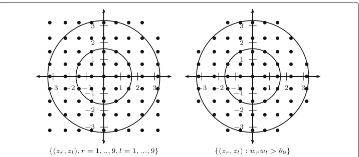
One can alternatively use a Cholesky decomposition, but as noted by Jäckel (2005), the spectral decomposition provides a better rotation of the sampling points, which makes the evaluation of the integral potentially more robust. Another issue is the waste of com-putation time. The two-dimensional standard normal density for example has circular level curves centered at the origin. Its mass is concentrated within circles of rays less than or equal to 3. However, the set of sampling points obtained by taking the cartesian prod-uct of one-dimensional sets of sampling points is a square in two dimensions. The mass at the points located at the extremities of the axes of the square is almost zero and does not contribute to the integral, which wastes computation time. One way to deal with this issue is to use what is called “pruning” (Jäckel 2005) which is a way of eliminating these non-important points. This can be done by rewriting the integral approximation as:
∞
−∞
∞
−∞ Ti
t=1
f(yit|ξi1,ξi2)g(ξi1,ξi2)dξi1dξi2≈ 1 π
R
r=1
R
l=1
I{wrwl>θR}wrwl Ti
t=1
×f(yit|az1r+bz2l,cz1r+dz2l)
where
θR=
w1w"R+1 2
#
R .
Using the MATLAB function mherzo.m written by Zhang and Jin (1996) I have generated 9-point one-dimensional Gauss-Hermite weights,wrand nodeszr(r=1,..,9).
Fig. 1An example showing the effect of pruning. The number of points is reduced from 81 on the left to the most heavily weighted 69 points on the right
not only reduce computation time but also provide better accuracy in the case of logistic regressions.
Alternatively, one can use theh-likelihoodmethod by Lee and Nelder (1996) and bypass the computation of the integral. In this case the random effects are treated as addi-tional parameters that are estimated with the other parameters. For panel data with a large number of units this method increases significantly the number of parameters to be estimated.
A Hidden Markov Model (M5)
One problem with the models already presented is that they do not allow the group mem-bership at timetto be dependent on the group membership at timet-1. When the groups are made of firms having the same financial status, one should note that several of the variables used in the literature to determine the presence or the absence of financial con-straints such as the firm’s size, the fraction of its assets that can be used as collateral, are likely to be time-dependent and as a result, the firm’s financial status at timetis poten-tially dependent on its status at timet-1. One way to capture this time dependence is to make the following assumption
p(wit=1)=p(wit=1|wit−1=j),j=1, 2.
Let
p(wit=l|wit−1=k)=iPkl,k=1, 2;l=1, 2.
I assume thatwitis an unobserved variable following a first order Markov chain on a
discrete state-space. The bivariate discrete-time process(Yit,Wit)whereYit|witis
inde-pendent, is a hidden Markov model (Cappé et al. 2005). Thus, the joint density for (Yit,Wit)is given by
f(yit,wit)=
p(wit=1|i(t−1))f(yit|wit=1) p(wit=2|i(t−1))f(yit|wit=2)
If, for a given firmi, the path of the chain is:{wi1=j1,wi2=j2,. . .,wiTi=jTi}, the joint
density for this firm would be
f(yi1,. . .,yiTi),(wi1=j1,. . .,wiTi =jTi)
=p(wi1=j1,. . .,wiTi=jTi)
×f(yi1,. . .,yiTi)|wi1=j1,wi2=j2,. . .,wiTi
=p(wi1=j1)p(wi2=j2|wi1=j1)×. . .
×p(wiTi=jTi|wi(Ti−1)=jTi−1) ×f(yi1|wi1=j1)×f(yiTi|wiTi=jTi).
Note that the total number of possible paths is 2Tifor firmi. Suppose that the initial
probability vector for firmiis
iπ=(iπ1,iπ2).
The joint density can be rewritten as
iπj1 ×iPj1j2×. . .×iPjTi−1jTi×f(yi1|wi1=j1)×. . .×f
yiTi|wiTi=jTi
=iπj1f(yi1|wi1=j1) Ti
t=2
iPjt−1jtf(yit|wit=jt).
The preceding is true if we know a priori the full path of the state variable,wit. If we
don’t, the joint density can be written as
2
j=1
iπjf(yi1|wit=j)
I(wi1=j) Ti
t=2 2
k=1 2
l=1
iPklf(yit|wit=l)
I(wit−1=k,wit=l)
.
The marginal density for firmifor the observed data is then
2
j1=1 . . .
2
jTi=1
iπj1iPj1j2×. . .×iPjTi−1jTi×f(yi1|wi1=j1)×. . .×f
yiTi|wiTi=jTi
.
If
λ(yit)=
f(yit|wit=1) 0
0 f(yit|wit=2)
,γit=
iP11 iP12
iP21 iP22
,
then the marginal density can be rewritten using vector-matrix operations (MacDonald and Zucchini 1997)
iπλ(yi1)γi2λ(yi2)×. . .×γiTiλ(yiTi)1=iπλ(yi1) T
t=2
γitλ(yit) 1, (16)
where1is a column vector of ones.
Parameters Estimation (EM Algorithm)
Letθ =iπ1,iP11,iP22,β1,β2
be the vector of parameters of the model. WithNfirms, the dimension of the vectorθis
dim(θ)=3N+2 dim(βi)
which is a large number of parameters. To reduce the number of parameters to be estimated, I assume that
then,
dim(θ)=3+2 dim(βi).
Thecomplete-data likelihoodis given by
Lc(θ)= N
i=1 ⎛ ⎝2
j=1
πjf(yi1|wit=j)
I(wi1=j) Ti t=2 2 k=1 2 l=1
Pklf(yit|wit=l)
I(wit−1=k,wit=l)
⎞ ⎠,
(17)
and thecomplete-data log-likelihoodis
lc(θ)=log(Lc(θ))= n
i=1 ⎛ ⎝2
j=1
I(wi1=j)log(πjf(yit|wi1=j))
+ Ti t=2 1 k=0 2 l=1
I(wi(t−1)=k,wit=l)log(Pklf(yit|wit=l))
⎞ ⎠
or
lc(θ)=log(Lc(θ))= n
i=1 ⎛ ⎝2
j=1
I(wi1=j)log(πjf(yit|wi1=j))
+ Ti t=2 2 k=1 2 l=1
I(wi(t−1)=k,wit=l)log(Pkl)
+ Ti t=2 2 k=1 2 l=1
I(wit=l)logf(yit|wit=l)
⎞ ⎠.
The intermediate quantity of EM is
Q(θ;θ)=Eθ(lc(θ)|T)
=
n
i=1 ⎛ ⎝2
j=1
Eθ"I(wi1=j)log(πjf(yit|wi1=j))|iTi
# + Ti t=2 2 k=1 2 l=1
Eθ"I(wi(t−1)=k,wit=l)log(Pkl)
# + Ti t=2 2 k=1 2 l=1
Eθ"I(wit=l)log(f(yit|wit =l))|iTi
#⎞⎠ .
To get the preceding expectation, onlyEθ(I(wit =j|iTi))andEθ(I(wi(t−1) =k,wit = l|iTi))need to be evaluated. Note that
EθI(wit =j|iTi)
=pwit=j|iTi,θ
EθI(wi(t−1)=k,wit=l|iTi)
=pwi(t−1)=k,wit=l|iTi,θ
p(wi(t−1)=k,wit=l|iTi,θ )
= p
wi(t−1)=k,wit=l,iTi;θ
f(iTi)
= p
wi(t−1)=k,wit=l,yi1,. . .,yi(t−1),yit, ..,yiTi;θ
f(yi1,. . .,yi(t−1),yit, ..,yiTi)
= p
yi1,. . .,yi(t−1),wi(t−1)=k;θ)×p(yit, ..,yiTi,wit=l|wi(t−1)=k,yi1,. . .,yi(t−1);θ
f(yi1,. . .,syi(t−1),yit, ..,yiTi) = αi(t−1)(k)×p
wit=l|wi(t−1)=k;θ×fyit, ..,yiTi|wit=l,wi(t−1)=k;θ
f(yi1,. . .,yi(t−1),yit, ..,yiTi)
= αi(t−1)(k)×iPklf(yit|wit=l)×f
yi(t+1), ..,yiTi|wit=l,wi(t−1)=k;θ
f(yi1,. . .,yi(t−1),yit, ..,yiTi)
= αi(t−1)(k)×iPklf(yit|wit =l)× ˇβit(l) f(yi1,. . .,yi(t−1),yit, ..,yiTi)
where
αit(k)=p(yi1,. . .,yit,wit=k)
ˇ
βit(k)=f(yi(t+1),. . .,yiTi|wit=k).
The EM algorithm for this model proceeds as follows:
1. Choose initial valuesθ0and,
2. Computep(wit=j|iTi;θ0)andp(wi(t−1)=k,wit=l|iTi;θ0)for each
observation,
3. Substitute the computed probability in the intermediate EM quantity(Q)(θ1,θ0),
4. Solve
θ1=argmax
θ Q(θ,θ0)
subject to:
2
j=1 πj=1
2
l=1
Pkl =1;k=1, 2
0≤πj≤1,j=1, 2.
5. Repeat step 2 after replacingθ0byθ1,
6. Keep going until convergence.
It should be noted that the forward-backward algorithm used to obtainαit(k)andβˇit(k)
is subject to numerical underflow. To avoid this problem the FORTRAN codes used for this algorithm apply the scaling method proposed by Rabiner (1989). The version of the EM algorithm just presented is also known as the Baum-Welch algorithm. Step 4 is called the M-step or maximization step. The Lagrangian for the problem is
L(θ,λ,λk;θ)=Q(θ;θ)+λ ⎛ ⎝1−2
j=1 πj
⎞ ⎠+2
k=1 λk
1−
2
l=1
Assume, as before, thatf(yit|wit=l)is the density function of the normal distribution. Then, n i=1 Ti t=1
logf(yit|wit=l)= −
1 2 n i=1 Ti t=1 lnπ−
n i=1 Ti t=1 lnσl−
1 2σl2
n i=1 Ti t=1
(yit−xiβl)2.
Let
$
p(wit=l|iTi;θ)yit=y
(l)
it
$
p(wit=l|iTi;θ)xit=x
(l) it
y(11l),. . .,y(1lT1) ,y(21l),. . .,y(nTl) n
=y(l)
x11(l),. . .,x1(lT1) ,x21(l),. . .,x(nTl)n =x(l),
then
p(wit=l|iTi;θ)logf(yit|wit=l)= −
1 2 n i=1 Ti t=2
p(wit=l|iTi;θ)ln(2π)
− n i=1 Ti t=2
p(wit=l|iTi;θ)lnσl
− 1
2σl2
y(l)−x(l)βl
y(l)−x(l)βl .
The first order conditions for the maximization problem are the following:
wrt:πj
n i=1p
wi1=j|iTi;θ
πj =λ
(18)
wrt:Pkl
n i=1
Ti
t=2p(wi(t−1)=k,wit=l|iTi;θ)
Pkl =λk
,k=1, 2;l=1, 2 (19)
wrt:βl x(l) x(l)βˆl=
x(l) y(l) (20)
wrt:σ2 − 1
2 n i=1 Ti t=2
pwit=l|iTi;θ
σ2
l
= 1
2σl4
y(l)−x(l)βl
y(l)−x(l)βl
(21)
wrt:λ
2
j=1
πj=1 (22)
wrt:λk
2
l=1
Pkl =1. (23)
Combining Eqs. (18) and (22) one gets
n i=1 2 j=1
p(wi1=j|iTi;θ)= n
j=0
ˆ
λπˆj
⇒
n
i=1 1= ˆλ
Thus,
ˆ
πj=
1 n
n
i=1
p(wi1=j|iTi;θ). (24)
Combining Eqs. (19) and (23)
n
i=1
Ti
t=2 2
l=1
pwi(t−1)=k,wit=l|iTi;θ
= ˆλk
2
l=1
ˆ
Pkl
⇒
n
i=1
Ti
t=2
pwi(t−1)=k|iTi;θ
= ˆλk,
which implies
ˆ
Pkl=
n
i=1 Ti
t=2p
wi(t−1)=k,wit=l|iTi;θ
n
i=1 Ti
t=2p
wi(t−1)=k|iTi;θ
. (25)
From Eq. (20) one gets
ˆ
βl =
x(l) x(l)
−1
x(l) y(l). (26)
From Eq. (21) one obtains
ˆ
σ2=
y(l)−x(l)βl
y(l)−x(l)βˆl
n i=1
Ti
t=2p(wit=l|iTi;θ)
. (27)
One main drawback with the HMM model with constant transition matrix is that the probability for a firm to move from one state to another does not depend on any observable, which is unrealistic for reasons considered in the case of the first model.
HMM Model with Time dependent Transition Matrix (M6)
To relax the constraint imposed on the preceding model by the constant transition prob-abilities, a transition matrix whose components are functions of some observables can be used. Suppose
wit=
1 ifw∗it >0,t=1,. . .,Ti;i=1,. . .,n
2 otherwise (28)
where
w∗it=zitγ +λ(wi(t−1)−1)−it;it∼N(0, 1) (29)
The preceding equation means that it is possible to predict the financial situation of firmiat timetusing its situation at timet-1 and some exogenous variableszit. Thus,
p(wit=1|wi(t−1)=1)=p(it≥zitγ)=(zitγ)
p(wit=2|wi(t−1)=2)=p(it<zitγ +λ)=1−(zitγ +λ),
the transition matrix is then
(zitγ) 1−(zitγ)
(zitγ +λ) 1−(zitγ +λ)
.
possible to use a probit or logit model for each row of the transition matrix. In fact, when the Markov chain has more than two states a multinomial probit or logit model would be the most convenient choice. However, for a chain with two states, the current specifi-cation appears to be better since it involves a smaller number of parameters and offers a nice way to test for time dependence by testing the hypothesisλ=0.
Parameters Estimation
The complete-data log-likelihood function looks the same as in the previous section. The only difference is that the transition probabilities depend now on the parametersγ andλ. As a result, instead of estimating the transition matrix, I will have to estimateγ andλ. Note that there are no closed form solutions for the first order conditions with respect toγ andλ. So, the M-step of the EM algorithm will include a Newton-Rapthon maximization step.
(γˆ,λ)ˆ =arg max (γ,λ)
n
i=1
Ti
t=2 2
k=1 2
l=1
Ewit
"
I(wi(t−1)=k,wit=l)log(iPkl);θ
# ,
whereiPkl,k= 1, 2;l =1, 2;i= 1, ..,nare given in the preceding transition matrix. The
HMM model presented in this section does not account for within group heterogeneity which opens the door for a possible extension.
Hidden Markov Model with Time Varying Transition Matrix and Random Effects (M7) Even though the groups are homogeneous with respect to the financial characteristics used to form them, there are still some unobserved characteristics with respect to which the firms within a given group can be considered to be heterogeneous. One such char-acteristic is the difference in management. To take account of this additional source of heterogeneity, I introduce an unobserved firm specific variable in each of the two components. Let
α1i= ¯x.iζ1+ξi1 α2i= ¯x.iζ2+ξi2
(30)
ξ1i
ξ2i ∼
N(0,) (31)
ξji (j=1,2) are random effects that are uncorrelated with xit and x¯.i. The conditional
expectations will be modeled such that
E(yit|xit,x¯it,ξji,wit=j)=xitβj+ ¯xitζj+ξji,j=1, 2. (32)
I also assume that the random effect is independent of the firm’s financial situation captured with the variablewit and that conditional on the random effects and{wit}T1i, investment is independent. The complete-data likelihood can be written as
Lc(θ)= n
i=1 ⎛ ⎝2
j=1
πjf(yi1|wit=j,ξij)I(wi1=j)
×
Ti
t=2 2
k=1 2
l=1
iPklf(yit|wit=l,ξij)
I(wit−1=k,wit=l)
h(ξ1i,ξ2i)
The complete-data log-likelihood is then
lc(θ)=log(Lc(θ))= n
i=1 ⎛ ⎝2
j=1
I(wi1=j)log(πjf(yit|wi1=j,ξij))
+ Ti t=2 2 k=1 2 l=1
I(wi(t−1)=k,wit=l)log(iPkl)
+ Ti t=2 2 k=1 2 l=1
I(wit =l)logf(yit|wit=l,ξij)
+ logh(ξi1,ξi2) ⎞ ⎠.
The intermediate EM quantity is given by
Q(θ;θ)=Eξ"Ewit(lc(θ)|iTi;θ)
# = n i=1 ⎛ ⎝2
j=1
Ewit
"
I(wi1=j)log
πj
|iTi;θ
#+Ti t=2 2 k=1 2 l=1
×Ewit
"
I(wi(t−1)=k,wit=l)log(iPkl)|iTi;θ
# + Ti t=1 2 k=1 2 l=1
×Ewit
"
I(wit=l)log(f(yit|wit=l,ξil))|iTi;θ #h(ξ
i0,ξi1|iTi)dξi0dξi1
+
log(h(ξi0,ξi1))h(ξi1,ξi2|iTi)dξi0dξi1
⎞ ⎠.
Closed-form solution for the maximization of the intermediate EM quantityQ(θ,θ) exists only for the first component. The other three components have to be maximized using a Newton-type method. Let the Lagrangian for the first component be
L(πj,ζ)= n
i=1 ⎛ ⎝2
j=1
Ewit
"
I(wi1=j)log(πj))|iT;θ
#⎞⎠
+ζ
⎛ ⎝1−2
j=1 πj
⎞ ⎠.
The first order conditions are
n
i=1
Ewit
"
I(wi1=j)|iT;θ #
= ˆζπˆj;j=1, 2 (33)
2
j=1
ˆ
πj=1. (34)
Thus, n j=0 n i=1
E"I(wi1=j)|iT;θ # = ˆζ 2 j=1 ˆ
πj. (35)
Using Eq. (34) in Eq. (35), I get
ˆ ζ= n j=0 n i=1 Ewit "
I(wi1=j)|iT;θ #
since 2
j=1
n
i=1
Ewit
"
I(wi1=j)|iT;θ#=
n
i=1 2
j=1
p(wi1=j|iT)=
n
i=1 1=n.
Thus
ˆ
πj=
1 n
n
i=1
Ewit
"
I(wi1=j)|iT;θ #
= 1
n n
i=1
p(wi1=j|iT)
= 1
n n
i=1
p(wi1=j,iT)
f(iT) =
1 n
n
i=1
p(wi1=j,iT|ξi1,ξi2)h(ξi1,ξi2)dξi1dξi2
f(iT|ξi1,ξi2)h(ξi1,ξi2)dξi1dξi2
= 1
n n
i=1
p(wi1=j,yi1|ξi1,ξi2))×f(yi2,· · ·,yiTi|wi1=j,ξi1,ξi2)h(ξi1,ξi2)dξi1dξi2 f(yi1,· · ·,yiTi|ξi1,ξi2)h(ξi1,ξi2)dξi1dξi2
= 1
n n
i=1
νit(j|ξi1,ξi2)βˇit(j|ξi1,ξi2)h(ξi1,ξi2)dξi1dξi2 2
j=1 νit(j|ξi1,ξi2)βˇit(j|ξi1,ξi2)h(ξi1,ξi2)dξi1dξi2 ,
where
νi1(j|ξi1,ξi2)=p(wi1=j,yi1|ξi1,ξi2)=p(wi1=j|ξi1,ξi2)f(yi1|wi1=j,ξi1,ξi2)
ˇ
βi1(j|ξi1,ξi2)=f(yi2,· · ·,yiTi|wi1=j,ξi1,ξi2)
=
2
k=1
f(yi2,· · ·,yiTi,wi1=j,wi2=k|ξi1,ξi2) p(wi1=j|ξi1,ξi2)
=
2
k=1
p(wi1=j|ξi1,ξi2)p(wi2=k|wi1=j,ξi1,ξi2)
p(wi1=j|ξi1,ξi2)
× f(yi2,· · ·,yiTi|wi1=j,wi2=k,ξi1,ξi2)
=
2
k=1 "
p(wi2=k|wi1=j,ξi1,ξi2)
× f(yi2|wi2=k,ξi1,ξi2)f(yi3,· · ·,yiTi|wi2=k,ξi1,ξi2)
#
=
2
k=1
iPjkf(yi2|wi2=k,ξi1,ξi2)βˇi2(k|ξi1,ξi2) .
Let
νit(j|ξi1,ξi1=p(wit=j,yit|ξi1,ξi1)
ˇ
βit(j|ξi1,ξi1)= 2
k=1
iPjkf(yi(t+1)|wi(t+1)=k,ξi1,ξi2)βˇi(t+1)(k) ,
then
νit(j)= (νit(j|ξi1,ξi2)h(ξi1,ξi2)dξi1dξi2
ˇ
βit(j)= βˇit(j|ξi1,ξi2)h(ξi1,ξi2)dξi1dξi2.
Hidden Markov Model with Time Varying Transition Matrix and endogeneity (M8) An alternative way of extending modelM6is to assume that the states of the Markov chain and the response variable are dependent. More precisely, we can assume
yit=
yit1=xitβ1+u1it, ifwit=1 yit2=xitβ2+u2it, ifwit=2
,
together with Eqs. (28), (29) and
it u1it
∼N
0 0
,
1 σ1 σ1 σ12
it u2it
∼N
0 0
,
1 σ2 σ2 σ22
.
The last distributional assumptions make the states of the Markov chains and the response variableyitinterdependent. The resulting model is an extension to the panel data
setting of a modified version of the model by Kim et al. (2008). The transition matrix of the current model uses less parameters and the correlations between the state-indicator variable and the component distributions are allowed to be different.
Parameters estimation
Because of the interdependence between the states of the Markov chains and the response variable, during the maximization step of the EM the parameters of the transi-tion matrix and the component distributransi-tions have to be estimated together. As a result, the EM algorithm does not have any computational advantage over a Newton-type algo-rithm applied to the marginal likelihood. The latter can be written as in Eq. (16) after some suitable transformation. Note that
f(yit|wit=1)=
f(yit,wit =1)
(zitγ +λ(wi(t−1)−1)) .
Thus, to evaluate this conditional density the current state and the previous state are both needed. The computation of the likelihood will require conditional densities that depend on the current state and the previous state. Since the transition matrix has two states, four conditional densities will result. To write the likelihood as in Eq. (16), the Markov chain has to be written as a four-state chain. LetWWitbe the new Markov chain
with state space
{11, 12, 21, 22}.
wwit equalskl is equivalent towi(t−1) equalskandwit equalsl. The transition matrix
associated to the new chain can be written as
γit=
⎡ ⎢ ⎢ ⎢ ⎣
itP11 itP12 0 0 0 0 itP21 itP22
itP11 itP12 0 0 0 0 itP21 itP22
⎤ ⎥ ⎥ ⎥ ⎦
Since the component densities now depend on the current state and the previous state, if the initial distribution of the old state-indicator variable (wit) is still the distribution