Fereshteh Poorahangaryan
1and Hassan Ghassemian
2*Abstract
This paper aimed to present a new method for the spectral-spatial classification of hyperspectral images, based on the idea of modified minimum spanning forest (MMSF). MMSF works on the obtained regions of pre-segmentation step that are considered as nodes of an image graph. In the proposed method, the image is first smoothed by the multiscale edge-preserving filter (MSEPF) and then the MMSF is built in each scale. Finally, all the classification maps of each scale are combined with a majority vote rule. The suggested method, named as MSEPF-MMSF, is performed on four hyperspectral images with different properties, and the experiments deal with the impacts of parameters of filter and the number of markers. The results demonstrate that the proposed method has improved the classification accuracies with respect to the previous methods.
Keywords:Edge-preserving filter, Hyperspectral images, Segmentation, Spectral-spatial classification, Minimum spanning forest
1 Introduction
Image processing and video analysis are one interesting topic in intelligent systems in recent years [1–3]. In hyper-spectral images, a vector with several hundreds of spec-trums is assigned to each spatial position. Such numbers are tantamount to the reflexive light spectrum. Such precious spectral information enhances the capability of recognizing physical material and other different objects. One of the valuable uses of hyperspectral images analysis is classification process through which a class is assigned to each image pixel. Hyperspectral image classification represents a hot research area [4–6]. However, the funda-mental problems are high dimension and limitation in number of training samples. In order to tackle the prob-lems, different dimension reduction methods [7–9] have been suggested. Extensive researches have been carried out into hyperspectral image classification, most of which only use spectral information. Methods such as neural networks [10], decision tree [11], kernel-based methods
[12], and support vector machine (SVM) [13] have been proposed in order to fulfill the goal. SVM works very well, specifically to limited training samples [13]. Image spatial resolution has been enhanced thanks to advances in the
technology of hyperspectral image equipment [14–24].
Therefore, if spatial information (the information obtained from pixel neighborhood) combined with spectral infor-mation, classification accuracy will increase. As a result, several numbers of spatial-spectral classification tech-niques have been introduced in recent years. In general, spatial-spectral classification methods can be divided into two groups. The first group is composed of methods based on a crisp neighborhood system such as the Markov random field (MRF) [14] and related gener-alized methods [15, 16]. These methods have achieved appropriate performance in classification. But if neigh-borhood pixels strongly depended on each other, the concept of neighborhood may not include effective samples. On the other hand, using a large neighbor-hood may cause computational problems [17]. The second group is composed of methods based on adaptive neighborhood. The morphology-based methods [18] and
the segmentation-based methods [19–24] fall in this
category. Although morphology-based methods are
* Correspondence:[email protected]
2Image Processing and Information Analysis Lab. Faculty of Electrical and
Computer Engineering, Tarbiat Modares University, Jalale Ale Ahmad Highway, P.O. Box 14115-111, Tehran, Iran
Full list of author information is available at the end of the article
instrumental tools for obtaining spatial information, the shape of the structuring element (SE) and computational complexity are still key issues in such classifications [18]. Segmentation is also a powerful tool for defining spatial dependency where, by this tool, an image can be divided into homogenous regions. Segmentation techniques ex-tract a large neighborhood for large regions. Meanwhile, small regions containing one or more pixels are not eliminated. Methods like watershed [19], clustering [20], hierarchical segmentation [21], and marker-controlled mentation methods [22, 23] have been presented for seg-mentation and classification of hyperspectral images. Meanwhile, marker-controlled segmentation methods such as SVM-MSF (SVM-minimum spanning forest) [22] and MSSC-MSF (multispectral-spatial classifier-MSF) [23] can decrease over-segmentation and increase classification ac-curacy more than other methods [21]. The SVM-MSF uses probability SVM and consequently MSF. The MSSC-MSF uses multispectral-spatial classification for marker selection, and MSF is built on the obtained markers. However, marker selection is still a fundamental challenge. In addition, applying an extra step for marker selection leads to an increase in computation time.
Spatial filtering has been recently used in researches into hyperspectral image processing and has shown its efficiency in this topic [24, 25]. The simplicity of under-standing this type of filters is their main advantage, and their complexity are low [24]. Filters like weighted mean filter (WMF) [24] and edge-preserving filter (EPF) [25] are utilized to reduce image noise, increase consistency of neighborhood pixels, and provide homogenous regions.
In this paper, we propose a combination of spatial filter and MSF segmentation method for spatial-spectral hyperspectral image classification. In most of the researches related to hyperspectral image processing, single-scale filtering has been taken into use. But single-scale spatial filters have no capability to describe different spatial struc-ture of the hyperspectral images. Therefore, a multiscale edge-preserving filter has been proposed and used in the mentioned hybrid scheme. Furthermore, a modified model of MSF has been proposed and used in the suggested scheme. Despite traditional MSF that operates at the pixel scale, our model operates at the regional scale, and this process leads to a decrease in computational time.
2 Multiscale edge-preserving filter
Gaussian filtering is one of the most common methods for smooth an image. In this method, the underlying assumption is that images change slowly over space. On the other hand, the assumption does not work at edges. Despite Gaussian filters, EPF preserves the edges. In order to cope with this issue, the bilateral filter as one type of EPFs can be used. The bilateral filter has had wide applications thanks to the advantage of preserving
edges up to now. There are two conditions where the pixels can be close to each other. They can have a nearby spatial location, or they have a similar spectral signature. The traditional filtering is a spatial domain filtering. The combination of both the spatial domain and range filtering is known as bilateral filtering.
Since the hyperspectral images may consist of information in different resolutions, one scale of the filtering cannot extract the significant information [25]. To overcome this challenge, we present a multiscale edge-preserving filter called MSEPF. The proposed MSEPF (denoted as H) is defined as follows:
H½Ip ¼ 1
Wp
X
qNσsGσsð∥p−q∥ÞGσrðIp−IqÞPq ð 1Þ
with
Nσs¼ð2σsþ1Þ ð2σsþ1Þ σs¼1; 2;…;Q: ð2Þ
Wp ¼
X
q∈NσsGσsðkp−qkÞGσr Ip−Iq
ð3Þ
wherepand qrepresent thep-th andq-th pixels; Pand
I are the input image and reference image, respectively; σsdenotes theσs-th level (scale) of the decomposition;Q
is the number of the scale;Nσs is a local window of size
(2σs+ 1)×(2σs+ 1) at the σs-th scale around pixel p; and
Wp is a normalization factor. Gσs and Gσr can be
obtained from Eqs. (4) and (5), respectively.
Gσsðkp−qkÞ ¼ exp −
p−q
k k
σ2 s
!
ð4Þ
Gσr Ip−Iq
¼ exp − Ip−Iq
2
σ2 r
!
ð5Þ
where the vectorspandqepitomize the spatial location of the image. Furthermore,IpandIqare the intensity values of the locationspandq, respectively, andPandIare the input image and the reference image, respectively.Gσs is a
spatial Gaussian function. The more the distance from the center, the less Gσs becomes. Gσr is a range Gaussian
function. According to Eq. (4), the increase in the intensity difference betweenIpandIqleads to the decrease in Gσr.
Parametersσsandσr, which are the standard deviations of
Gaussian functions Gσs and Gσr, respectively, determine
the amount of filtering for the imageI[25].
3 Modified minimum spanning forest
For constructing a minimum spanning forest (MSF), a B-band hyperspectral image is given, which can be considered as a set ofn-pixel vectors X= {xj∈RB,j= 1, 2,…, n}.V andE are the sets of vertices and edges, respectively, and
a vertexv∈Vand each edgeeij∈Econnects two verticesi and jto each other. A non-zero weightwi,jis assigned to each edge. In order to compute weights of edges, spectral angle mapper (SAM) and L1 vector norm can be used [22]. Generation of an MSF on an image is performed as the following steps:
Convert image to graph according to the abovementioned way.
Compute weights of edges.
Add additional verticesti,i= 1,…,m, corresponding tom-selected markers.
Link per additional vertextito the pixels
representing a markeriby the zero-weighted edge and construct a new graph [22].
An MSF in G is included in the minimum spanning
tree of the graph, and every tree is grown on a vertexti;
when the vertex r is taken away, the MSF is produced.
Prim’s algorithm is employed for generating the MSF;
for more details, please see [22].
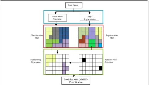
The modified MSF (MMSF) as a part of the overall flowchart of the proposed spectral-spatial classifica-tion method is shown in Fig. 1. As shown in Fig. 1,
Fig. 2Flowchart of the proposed spectral-spatial classification method (MSEPF-MMSF)
the image is firstly pre-segmented. So, the image is segmented to many small regions regarded as the nodes of MMSF. Compared to traditional MSF, the MMSF algorithm is presented in a smaller number of nodes and edges. On the other hand, a pixel-wised classification is performed. After the mentioned steps,
Nm pixels are chosen randomly. One region is
speci-fied for each selected pixel based on the pre-segmentation map. Subsequently, all the pixels of a region are appointed to the class with the highest frequency according to the result of the pixel-wised classifier in the given region. These regions are regarded as markers for MMSF construction. Also, a seg-mentationSis a division ofVinto regions such that each
region R∈S accords with a connected component in a
graphG′= (V,E′), whereE′∈E. The differences between the two regionsR1, R2⊂ Vcan be obtained by the mini-mum weight edge linking the two regions. That is,
w Rð 1;R2Þ ¼ min w vi;vj
vi∈R1;vj∈R2; vi;vj
∈E
and w vi;vj
¼wij
ð6Þ
w(R1, R2) = ∞ is allowed if no edge links R1 and R2. According to this measure, the algorithm will combine
two regions even though there is an edge with a low weight between them.
4 Proposed spectral-spatial classification method This section introduces a new spectral-spatial classifica-tion scheme for hyperspectral images. The overall flow-chart of the proposed spectral-spatial classification method (MSEPF-MMSF) is given in Fig. 2.
The MSEPF-MMSF is composed of the following three main steps: (1) preprocessing using MSEPF, (2) spatial-spectral classification of each individual scale of filtering using MMSF, and (3) majority vote rule for class decision.
There is a B-band hyperspectral image X = {xj ∈ RB, j = 1, 2, …, n} at the input. At first, the hyperspectral image is smoothed by multiscale bilateral filter defined in Section 2. At this point, the controversial issue is the
reference image selection, I. In order to tackle this
problem, principal component analysis (PCA) is applied because the optimum portrayal of the image is presented in the mean-squared sense. Original hyperspectral image
undergoes dimension reduction via PCA, and the firstr
principal components are chosen as the reference image for the bilateral filter. The value ofrcan be automatically selected by analyzing the eigenvalues of scatter matrices computed from the PCA [26]. In this step, we haveQ -fil-tered images. A spectral-spatial classification using MMSF is done in each individualQscale. We propose to use an
(a)
(b)
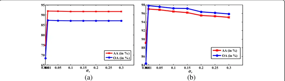
Fig. 4Analysis of the influence of the parameterσr.aIndian Pines image.bPaviaU image
(a)
(b)
SVM classifier for pixel-wised classification, which is strongly suitable for hyperspectral data classification [13]. In the pre-segmentation stage, we implemented watershed since it detects good boundaries and retains small differ-ences within the objects. Typically, the watershed trans-formation is used for a one-band image. There are several ways for generalizing this technique to an r-band hyper-spectral image [19].
In the final step, the classification maps of each individual scale are combined with a maximum vote decision rule and the final classification map is obtained. At this step of the algorithm, there areQspectral-spatial
classification maps corresponding to the Q scale of the
filtering step. The majority vote procedure is described
in the following way: For each pixel, a 1 × Q vector is
considered based on assigned classes in Q
spectral-spatial classification maps. In addition, the pixel is allo-cated to the highest frequency class. Every pixel of the image undergoes the abovementioned procedure. So the final classification map is acquired.
5 Results and discussion
The experimental study is done to indicate the perform-ance of the proposed spectral-spatial classification scheme. In this section, the experimental data sets are introduced and two various experiments are explained.
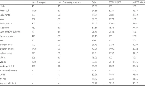
Table 1Information classes, number of training samples, and classification accuracy for the Indian Pines
No. of samples No. of training samples SVM SSEPF-MMSF MSEPF-MMSF
Alfalfa 46 15 95.65 100 100
Corn-notill 1428 50 64.85 80.31 86.55
Corn-mintill 830 50 61.57 91.81 90.72
Corn 237 50 86.08 98.73 100
Grass-pasture 483 50 92.55 95.86 94.62
Grass-trees 730 50 87.81 98.36 97.95
Grass-pasture-mowed 28 15 96.43 96.43 100
Hay-windrowed 478 50 99.16 100 100
Oats 20 15 100 100 100
Soybean-notill 972 50 66.46 87.74 88.79
Soybean-mintill 2455 50 47.94 84.95 85.38
Soybean-clean 593 50 71.5 93.57 92.22
Wheat 205 50 99.02 100 100
Woods 1265 50 83.32 96.13 97.15
Buildings-G-T-D 386 50 71.76 99.22 98.96
Stone-steel-towers 93 50 91.4 100 100
AA (%) – – 82.21 94.87 95.64
OA (%) – – 69.79 90.31 91.45
Kappa coefficient – – 66.27 89.18 90.32
(a)
(b)
In the first experiment, two well-known data sets includ-ing the non-urban data set (e.g., Indian Pines) and urban data set (e.g., PaviaU) are used. The effectiveness of
parameters (Nm, σr, Q) of the proposed method is
analyzed, and their optimal values are extracted. Also, the classification results and comparison with other methods are given. In the second experiment, the proposed method using the extracted optimal values is applied on two other data sets including Botswana and SalinasA. In this experi-ment, it is demonstrated that the good classification accuracies for various images will be achieved with the presented parameter setting. In addition, the classification results and discussion are presented.
5.1 Data sets
Four well-known hyperspectral data sets, i.e., the Indian Pines, the University of Pavia, the Salinas, and Botswana, go under the classification approach. The Indian Pines image capturing the agricultural Indian Pine test site of north-western Indiana was recorded by the AVIRIS sensor. This image contains 220 bands ranging from 0.4 to 2.5 μm with a spatial resolution of 20 m per pixel. It consists of 145 × 145 pixels and contains 16 classes. Twenty water absorption bands were removed before ex-periments (the removed bands are [104–108], [150–163], and 220). The ROSIS-03 satellite sensor captured an image of an urban area surrounding the University of Pa-via. This image is called PaviaU. The image is with the size 610 × 340 pixels and has 115 bands ranging from 0.43 to 0.86 μm with a spatial resolution of 1.3 m per pixel. In addition, the 12 most noisy channels were removed before experiments. Nine classes are considered for this image. The Salinas image was recorded by the AVIRIS sensor over Salinas Valley, CA, USA. This data set has 224 bands
in the wavelength range 0.4–2.5 μm with the size
512 × 217. The bands of [108–112], [154–167], and 224 are eliminated because of the water absorption bands, and
204 bands with a spatial resolution of 3.7 m per pixel are applied in our study. A subset of this image, named as SalinasA, is used. It is with the size 86 × 83 pixels, located in the [591–678] × [158–240] of Salinas Valley, containing six classes. The Botswana data set was recorded by the Hyperion sensor over Okavango Delta, Botswana. It
contains 242 bands covering the 400–2500 nm with a
spatial resolution of 30 m per pixel. The noisy bands ([10–55, 82–97, 102–119, 134–164, 187–220]) were removed, and the remaining 145 bands were used for experiments. This data set consists of 14 identified classes.
5.2 First experiment
In the used filters, the parameters σs and σr represent
the filtering size and blur degree, respectively. In addition, the numbers of Nminfluence the classification accuracy. In order to indicate the influence ofNm, four
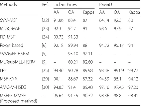
Table 3Average accuracy (AA), overall accuracy (OA), and kappa
for some segmentation-based and filter-based methods on Indian Pines and Pavia University data sets
Methods Ref. Indian Pines PaviaU
AA OA Kappa AA OA Kappa
SVM-MSF [22] 91.06 88.4 87 84.14 92.3 80
MSSC-MSF [23] 92.3 94.2 91 98.6 97.9 97
RD-MSF [24] 93.73 91.33 – – – –
Pixon based [6] 92.18 89.94 88 94.72 95.17 94
SVMMRF-HSRM [5] – 93.10 92.11 – – –
MLRsubMLL-HSRM [5] – 80.21 82.60 – – –
EPF [25] 94.46 90.28 89.98 98.38 99.09 98.77
MSF-KNN [29] 90.1 88.67 87.32 94.39 95.1 94.12
AMG-M-HSEG [30] 94.83 91.4 89.48 97.18 97.45 97.23
MSEPF-MMSF (Proposed method)
– 95.64 91.45 90.32 98.36 98.8 98.41
Table 2Information classes, number of training samples, and classification accuracy for the PaviaU
No. of samples No. of training samples SVM SSEPF-MMSF MSEPF-MMSF
Asphalt 6631 548 82.17 99.14 99.2
Meadows 18,649 540 87.25 97.28 99.23
Gravel 2099 392 81.23 95.95 95.43
Trees 3064 524 93.21 98.66 96.28
Metal sheets 1345 265 99.78 99.93 100
Bare soil 5029 532 91.05 99.54 99.8
Bitumen 1330 375 89.4 99.25 100
Bricks 3682 514 85.17 97.66 98.18
Shadows 947 231 99.89 99.79 97.36
AA (%) – – 89.9 98.57 98.36
OA (%) – – 87.6 99.18 98.8
different values have been determined, i.e., 0.2Nr, 0.4Nr, 0.6Nr, and 0.8Nr.
Nrsymbolizes the number of regions in the
segmenta-tion map obtained from the watershed. While the impact of analysis of the Nm is being analyzed, σr and σs are
supposed to be 0.2 and 3, respectively. The evolution of the overall accuracy (OA) and average accuracy (AA)
against the Nm for Indian Pines and PaviaU data set
is presented in Fig. 3. With an increase in Nm, the
classification accuracies increase until a zenith point is obtained. Reaching the maximum amount, the clas-sification accuracies initiate to reduce up to the SVM results. This figure shows that the highest amount of accuracy values is obtained whenNmis 0.4Nrand 0.6Nrfor the two abovementioned data sets, respectively. Although astounding, this difference of optimal value forNmcan be explained. In the non-unban data set, e.g., Indian Pines image, the objects are pretty wide and usually well delim-ited. So, though it is not high, the number ofNmwill be a fairly accurate classification. However, the PaviaU image in-cludes a lot of small regions. Thus, there should be enough
number of Nm in order to statistically have more
oppor-tunity to get at least one marker in each various region of the image. In conclusion, there is a higher amount of optimal value forNmcompared to the other images.
The impact ofσrand σson the classification efficiency
is investigated in Figs. 4 and 5, respectively. Nm is fixed
to be the optimal value and σs equals 3 during the
analysis of the effect of σr. In Fig. 4a, b, we can see the
evolution of the AA and OA against σr. Seven different
modes, i.e., 1, 2, …, 7, are considered so as to show the influence ofσs. Figure 5a, b shows the changes of
classi-fication accuracies as a function ofσsfor two data.
From Fig. 5, it is concluded that the optimal values of
σs are 4 and 2 for the Indian Pines and PaviaU images,
respectively. The results support that these parameters cannot be too small or too large. If the filtering size and blur degree, i.e., σs and σr, are too large, there may be a
dramatic decrease in the average classification accuracy that may over-smooth the maps. So, those small-scale objects may be misclassified. Likewise, a very small filtering size or blur degree is also unsatisfactory for the
(a)
(b)
(c)
(d)
Fig. 7PaviaU image.aGround truth data.bPixel-wised classification map using SVM.cClassification map obtained by SSEPF-MMSF.
dClassification map obtained by MSEPF-MMSF
(a)
(b)
(c)
(d)
Fig. 6Indian Pines image.aGround truth data.bPixel-wised classification map using SVM.c Classification map obtained by SSEPF-MMSF.
proposed method since it connotes that only very limited local spatial information is used in the filtering process. Hereafter, the optimal values of σr and Nm are
employed in each image. In our previous method [27], single-scale edge-preserving filter (SSEPF) is applied. Then, spatial-spectral classification is constructed using MMSF. Thus, this method is called SSEPF-MMSF. In SSEPF-MMSF, we used optimal values of both ofσsandσr,
which are obtained from the experiment. In MSEPF-MMSF (this work), seven values from 1 to 7 ofσsare used
and construction of MMSF is repeated for each scale. The final classification label for each pixel is achieved by com-bining the multiple results via majority voting.
Tables 1 and 2 present the classification results for the two mentioned data sets. These tables show the com-mon classification indexes, e.g., average accuracy (AA), overall accuracy (OA), and kappa coefficient. Further-more, the classification accuracy of each class obtained by pixel-wised classifier and proposed methods are given. In these tables, the results of Monte Carlo simula-tions (after 10 runs) are reported. Training samples were randomly selected from the Ground truth data.
It can be understood that through using the proposed classifier, the classification accuracies are increased signifi-cantly when compared to the pixel-wised classification. In the Indian Pines, the MSEPF-MMSF increases the classifi-cation accuracy compared to the SVM classifier by about
13%. In the PaviaU data set, the OA is improved by 18% points and the AA by 12.13% points. It is worth noting that the SSEPF-MMSF classifier is presented with better performance than the MSEPF-MMSF classifier in the PaviaU. In the following, the reason for this result is explained. PaviaU data set contained many small areas such as shadow.
As can be seen from Table 3, the MSEPF-MMSF improves all of the accuracies than SSEPF-MMSF except for the classes shadows and trees. These classes contained the very small object. Furthermore, at the small scale of filtering, the SSEPF-MMSF has been proven to be more suitable for classification of such classes. Increasing the scale of filtering may over-smooth the maps, and thus, such classes may be misclassified. In the MSEPF-MMSF method, the results of different scales are combined using majority voting. Because these classes are not on a large scale with good results, the classification accuracy of the MSEPF-MMSF method is lower than that of SSEPF-MMSF. As a result, the MSEPF-MMSF might not be the most suitable one for classifying such images that contain very small objects. Considering the obtained results, it is clear that the final classification results are the best ones although the initial pixel-wised classifier does not perform very well. The adjacent pixel consistency increases and provides more homogeneous objects brought on by the filtering step. Thus, much smoother classification maps
Fig. 9Comparison between the proposed classifier and some state-of-the-art methods for PaviaU
are obtained. The proposed multiscale method can de-scribe different spatial structures, and hence, our proposed algorithm has higher classification accuracy than the SSEPF-MMSF, except for the PaviaU image. It should be noted that the classification results of SSEPF-MMSF and MSEPF-MMSF are so close together for the PaviaU data set. It can be concluded that the SSEPF-MMSF method has been proven to be more adaptable for the classification of the urban area, but the MSEPF-MMSF method is suitable for the non-urban area. The Ground truth data, the classification maps of pixel-wised classifier, and our proposed classifiers (SSEPF-MMSF and MSEPF-MMSF) for the two data sets are shown in Figs. 6 and 7. These figures show that the classification map represented by the SVM is not very well because it is still possible to see some
noisy pixels, whereas the proposed classifiers provide a smoother classification map.
Although the MSEPF-MMSF method has good
performance, the primary problem of this method is
determining the optimal values for the parameters Nm,
σr, and Q. Based on the performed experiments, default
values can be suggested for these parameters. For σr, it
can be shown that with increasing values ofσr, the
com-putation time is increased without giving better results. Therefore, we suggest setting this parameter to 0.05. For
Q, it has been observed in our experiments that after the seventh scale, there is no significant improvement in the accuracy values. We suggest setting this parameter to 7.
The determination of the optimal value of Nm is not a
simple task. It has been indicated that for the images with a big region (such as Indian Pines), the optimal
Table 5Information classes, number of training samples, and classification accuracy for the Botswana
No. of samples No. of training samples SVM SSEPF-RSMSF MSEPF-RSMSF
Water 270 23 100 99.63 100
Hippo grass 101 23 89.11 100 100
Floodplain grasses1 251 25 100 100 100
Floodplain grasses2 215 23 93.49 100 100
Reeds1 269 23 85.5 96.65 98.88
Riparian 269 23 84.76 100 100
Firescar2 259 23 97.68 100 100
Island interior 203 23 97.04 100 100
Acacia woodlands 314 24 92.04 100 100
Acacia shrublands 248 23 95.56 100 100
Acacia grasslands 305 23 90.49 99.67 99.67
Short mopane 181 23 90.61 100 100
Mixed mopane 268 23 92.16 100 100
Exposed soils 95 23 100 100 100
AA (%) – – 93.46 99.7 99.89
OA (%) – – 93.23 99.66 99.88
Kappa coefficient – – 92.66 99.63 99.87
OA (%) – – 96.59 99.4 99.48
value ofNmis 40% of the total number of regions of the pre-segmented image. However, for the image such as PaviaU, which is composed of many small areas, the
optimal value of Nm is 60% of the total number of
regions of the pre-segmented image. Thus, the user should have background knowledge of the image in order to obtain the best results.
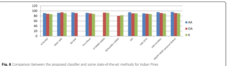
In Table 3 and Figs. 8 and 9, the proposed classifier is compared with classification results obtained with some state-of-the-art methods for Indian Pines and PaviaU data sets. These methods include construction MSF on markers obtained from probability SVM (SVM-MSF) [22], classification by building an MSF on markers extracted from multispectral-spatial classifier (MSSC-MSF) [23], classification by construction of an MSF on random markers (RD-MSF) [28], classification by con-struction of an MSF on extracted markers of KNN (MSF-KNN) [29], classification by the algebraic multi-grid method and hierarchical segmentation algorithm (AMG-M-HSEG) [30], edge-preserving filter (EPF)-based classification [25], adaptive pixon extraction tech-nique [6], and two types of hierarchical statistical region merging (HSRM) [5] for Indian Pines and PaviaU data sets. The classification results obtained by different approaches for the Indian Pines data set with 50 random training samples per class (15 for smaller classes) are given. Furthermore, we reported the classification accuracy of the mentioned schemes for PaviaU data set with 3921 total training samples. The MSEPF-MMSF method can describe different spatial structures, and hence, our proposed algorithm has higher classification accuracy than the other
methods. Although not satisfying, the obtained accuracies of the proposed methods for PaviaU data set are so close to the results obtained by the MSSC-MSF method [23]. Similarly, by comparing the result of our model and EPF [25], we can see that our result for Indian Pines is better than EPF [25], and for PaviaU, both results are so close. Moreover, in [28], the EPF [25] was compared with the sin-gle scale of our model (SSEPF-MMSF), and the results ex-plain that for PaviaU, the SSEPF-MMSF works better [27].
We note that the obtained results of each models depend on the parameter setting and the researchers often insert the best parameters for the results [5, 6, 22–24].
Next, we demonstrate the marker selection process of MSF-based approaches [22, 23] from the point of view of time-consuming.
Marker selection is the main problem when an MSF is created. Even though showing a good performance for hyperspectral image analysis, using a marker-controlled approach of supervised segmentation is challenging due to the issue of marker selection. The SVM-MSF method [22] requires the computation of an SVM probabilistic map. In RD-MSF [24] and in the proposed methods since these methods do not need the probability esti-mates for selection of the markers, this time-consuming step is not used. The random selection of the markers in the proposed methods is at a higher speed compared to the marker selection done by connected component ana-lysis [22]. The MSSC-MSF [23] approach is required to apply multispectral-spatial classifier in the marker selec-tion step. Thus, the marker selecselec-tion strategy is more time-consuming in comparison with the one that is used
(a)
(b)
(c)
(d)
Fig. 11Botswana image.aGround truth data.bPixel-wised classification map using SVM.c Classification map obtained by SSEPF-MMSF.
dClassification map obtained by MSEPF-MMSF
Fig. 10SalinasA image.aGround truth data.bPixel-wised classification map using SVM.cClassification map obtained by SSEPF-MMSF.
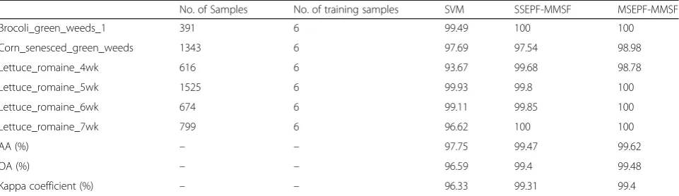
5.3 Second experiment
In order to confirm the discussion of algorithm perform-ance based on the provided parameter setting, the proposed algorithm (MSEPF-MMSF) is applied on two other well-known hyperspectral images including SalinasA and Botswana. In this experiment, the parameters of the algorithms are set at the optimal values extracted from the first experiment. In Tables 4 and 5, the number of training and test samples of each class and the classification accur-acies for these data sets are given. In order to visualize the analysis, the obtained classification maps of the SVM clas-sifier and the abovementioned clasclas-sifiers (SSEPF-MMSF and MSEPF-MMSF) are given in Figs. 10 and 11. It is clear that the obtained classification map of MSEPF-MMSF is less noisy than the other two classification maps. More-over, the classification accuracies are enhanced using the MSEPF-MMSF method. For example, the OA is improved by 6.65% and the AA by 6.43% when compared to the SVM classification for the Botswana data set. The result indicates that the good classification accuracies for the different images will be achieved with the use of the extracted optimal values of the parameters.
The following table represents McNemar’s test [31]
results for the Botswana data set (Table 6). The result of
McNemar’s test indicates the using of MSEPF-MMSF
improves confidence of classification than SSEPF-MMSF. MSEPF-MMSF will remove the statistical fluctu-ations of the classification. So, the efficiency and the robustness of the results will be enhanced. In fact, rather than preserving only the best classification result, the results of all classifiers even the unsuccessful ones are kept. The combination of these rich information using the majority voting decision rule provides the comple-mentary spectral-spectral information and improves the classification accuracy. Thus, the confidence of classification will be improved. The results of the McNemar test for the Botswana image are given be-cause it has a bigger size than the other researched images.
6 Conclusions
In this paper, a new method is proposed for spectral-spatial classification by the combination of modified
itional MSF because of the reduction in the number of nodes and edges. In addition, the marker-based ap-proach of supervised segmentation which suffers from an issue of marker selection does not exist in this new method. The proposed method is also compared to some state-of-the-art methods. The results indicate that the proposed method has good performance in hyper-spectral image classification. It is worth mentioning that the primary problem of the proposed method is deter-mining the optimal values for the related parameters and that an automatic determination of these parameters would be a very interesting direction for future research.
Acknowledgements
The authors would like to thank the management of the Department of Electrical Engineering, Science and Research Branch, Islamic Azad University, Tehran, Iran, for providing us with the infrastructure to complete the research work.
Funding
This work is supported by the Science and Research Branch of Islamic Azad University, Tehran, Iran.
Availability of data and materials
Not applicable.
Authors’contributions
HG is the corresponding author. FP is the first author. Both authors made the algorithm and experiments. Both authors read and approved the final manuscript.
Authors’information
Hassan Ghassemian received his Electronics and Communication degree from Telecommunication College, Tehran, Iran, in 1980. He later got an M.E degree in Communication Engineering from the School of Electrical and Computer Engineering, Purdue University, USA, in 1984. He completed his PhD from the same university in the year 1988. His current research interests include Signal and Information Processing Multisource Image Analysis (Image and Information fusion), Pattern Recognition Remote Sensing System Engineering (Hyperspectral Image Analyses), and Biomedical Signal and Image Processing. He has published more than 100 research papers in reputed journals and conference proceedings. Fereshteh Poorahangaryan received her BE degree in Electronics Engineering from Amirkabir University, Iran, in 2006 and ME in Electronics Engineering from Guilan University, Iran, in 2009. She completed her PhD from the Science and Research Branch of Islamic Azad University, Iran, 2017. Her research interests include image processing, computer vision, and medical image analysis.
Competing interests
The authors declare that they have no competing interests.
Publisher’s Note
Author details
1Department of Electrical Engineering, Science and Research branch, Islamic
Azad University, Tehran, Iran.2Image Processing and Information Analysis
Lab. Faculty of Electrical and Computer Engineering, Tarbiat Modares University, Jalale Ale Ahmad Highway, P.O. Box 14115-111, Tehran, Iran.
Received: 8 June 2017 Accepted: 23 October 2017
References
1. C Yan, H Xie, D Yang, J Yin, Y Zhang, Q Dai, Supervised hash coding with deep neural network for environment perception of intelligent vehicles. IEEE Trans. Intell. Transp. Syst99, 1–12 (2017).
doi: 10.1109/TITS.2017.2749965
2. C Yan, Y Zhang, J Xu, F Dai, J Zhang, Q Dai, F Wu, A highly parallel framework for HEVC coding unit partitioning tree decision on many-core processors. IEEE Signal Process Lett21(5), 573–576 (2014).
doi: 10.1109/LSP.2014.2310494
3. C Yan, Y Zhang, J Xu, F Dai, J Zhang, Q Dai, F Wu, Efficient parallel framework for HEVC motion estimation on many-core processors. IEEE Trans. Circuits Syst. Video Technol24(12), 2077–2089 (2014). doi: 10.1109/TCSVT.2014.2335852 4. X Ma, J Geng, H Wang, Hyperspectral image classification via contextual
deep learning. EURASIP J Image Video Process2015, 20 (2015). doi: 10.1186/s13640-015-0071-8
5. M Golipour, H Ghassemian, F Mirzapour, Integrating hierarchical segmentation maps with MRF prior for classification of hyperspectral images in a Bayesian framework. IEEE Trans Geos Remote Sens54(2), 805–816 (2016). doi: 10.1109/TGRS.2015.2466657
6. A Zehtabian, H Ghassemian, An adaptive pixon extraction technique for multispectral/hyperspectral image classification. IEEE Geos. Remote Sens. Lett12(4), 831–835 (2015). doi: 10.1109/LGRS.2014.2363586
7. L Zhang, D Tao, X Huang, Tensor discriminative locality alignment for hyperspectral image spectral-spatial feature extraction. IEEE Trans. Geos. Remote Sens51(1), 242–256 (2013). doi: 10.1109/TGRS.2012.2197860 8. M Imani, H Ghassemian, Ridge regression-based feature extraction for
hyperspectral data. Int. J. Remote Sens36(6), 1728–1742 (2016). doi: 10.1080/01431161.2015.1024894
9. A Kianisarkaleh, H Ghassemian, Nonparametric feature extraction for classification of hyperspectral images with limited training samples. ISPRS J. Photogramm. Remote Sens119, 64–78 (2016).
doi: 10.1016/j.isprsjprs.2016.05.009
10. Y Zhong, L Zhang, An adaptive artificial immune network for supervised classification of multi-/hyperspectral remote sensing imagery. IEEE Trans Geos Remote Sens50(3), 894–909 (2012). doi: 10.1109/TGRS.2011.2162589 11. HR Bittencourt, DA de Oliveira Moraes, V Haertel, inProceedings of IEEE
International Geoscience Remote Sensing Symposium. A binary decision tree classifier implementing logistic regression as a feature selection and classification method and its comparison with maximum likelihood (2007), pp. 1755–1758. doi: 10.1109/IGARSS.2007.4423159
12. G Camps-Valls, L Bruzzone, Kernel-based methods for hyperspectral image classification. IEEE Trans. Geos. Remote Sens43, 1351–1362 (2005). doi: 10.1109/TGRS.2005.846154
13. G Mountrakis, J Im, C Ogole, Support vector machines in remote sensing: a review. ISPRS J. Photogramm. Remote Sens66(3), 247–259 (2011). doi: 10.1016/j.isprsjprs.2010.11.001
14. Q Jackson, D Landgrebe, Adaptive bayesian contextual classification based on Markov random fields. IEEE Trans Geos Remote Sens40(11), 2454–2463 (2002). doi: 10.1109/TGRS.2002.805087
15. G Zhang, X Jia, Simplified conditional random fields with class boundary constraint for spectral-spatial based remote sensing image classification. IEEE Geos. Remote Sens. Lett9(5), 856–860 (2012). doi: 10.1109/LGRS.2012.2186279
16. P Ghamisi, JA Benediktsson, MO Ulfarsson, Spectral–spatial classification of hyperspectral images based on hidden Markov random fields. IEEE Trans Geos Remote Sens52(5), 2565–2574 (2014). doi: 10.1109/TGRS.2013.2263282 17. M Fauvel, Y Tarabalka, JA Benediktsson, J Chanussot, JC Tilton,
Advances in spectral-spatial classification of hyperspectral images. Proc. IEEE101(3), 652–675 (2013). doi: 10.1109/JPROC.2012.2197589 18. P Ghamisi, M Dalla Mura, JA Benediktsson, A survey on spectral–spatial
classification techniques based on attribute profiles. IEEE Trans Geos Remote Sens53(5), 2335–2353 (2015). doi: 10.1109/TGRS.2014.2358934
19. Y Tarabalka, J Chanussot, JA Benediktsson, Segmentation and classification of hyperspectral images using watershed transformation. Pattern Recogn
43(7), 2367–2379 (2010). doi: 10.1016/j.patcog.2010.01.016
20. Y Tarabalka, JA Benediktsson, J Chanussot, Spectral spatial classification of hyperspectral imagery based on partitional clustering techniques. IEEE Trans. Geosci. Remote Sens47(9), 2973–2987 (2009). doi: 10.1109/TGRS.2009.2016214 21. Y Tarabalka, JC Tilton, JA Benediktsson, JA Chanussot, A marker-based
approach for the automated selection of a single segmentation from a hierarchical set of image segmentations. IEEE J Sel Top Appl Earth Obs Remote Sens5(1), 262–272 (2012). doi: 10.1109/JSTARS.2011.2173466 22. Y Tarabalka, J Chanussot, JA Benediktsson, Segmentation and classification
of hyperspectral images using minimum spanning forest grown from automatically selected markers. IEEE Trans. Syst. Man Cybern. B Cybern
40(5), 1267–1279 (2010). doi: 10.1109/TSMCB.2009.2037132
23. Y Tarabalka, JA Benediktsson, J Chanussot, JC Tilton, Multiple spectral-spatial classification approach for hyperspectral data. IEEE Trans. Geosci. Remote Sens48(11), 4122–4132 (2010). doi: 10.1109/TGRS.2010.2062526
24. A Kianisarkaleh, H Ghassemian, Spatial-spectral locality preserving projection for hyperspectral image classification with limited training samples. Int. J. Remote Sens37(21), 5045–5059 (2016). doi: 10.1080/01431161.2016.1226523 25. X Kang, S Li, JA Benediktsson, Spectral-spatial hyperspectral image
classification with edge-preserving filtering. IEEE Trans. Geosci. Remote Sens
52(5), 2666–2677 (2014). doi: 10.1109/TGRS.2013.2264508
26. JA Benediktsson, P Ghamisi,Spectral-spatial classification of hyperspectral remote sensing images(Artech House, Norwood, 2015)
27. F Poorahangaryan, H Ghassemian,Minimum spanning forest based approach for spatial-spectral hyperspectral images classification, 2016 Eighth
International Conference on Information and Knowledge Technology (IKT)
(2016), pp. 116–121. doi: 10.1109/IKT.2016.7777749
28. K Bernard, Y Tarabalka, J Angulo, J Chanussot, JA Benediktsson, Spectral– spatial classification of hyperspectral data based on a stochastic minimum spanning forest approach. IEEE Trans. Geosci. Remote Sens21(4), 2008–2021 (2012). doi: 10.1109/TIP.2011.2175741
29. RD da Silva, H Pedrini, Hyperspectral data classification improved by minimum spanning forests. J. Appl. Remote. Sens10(2), 025007 (2016). doi: 10.1117/1.JRS.10.025007
30. H Song, Y Wang, A spectral-spatial classification of hyperspectral images based on the algebraic multigrid method and hierarchical segmentation algorithm. Remote Sens8(4), 296 (2016). doi: 10.3390/rs8040296