R E S E A R C H
Open Access
Cascaded reconstruction network for
compressive image sensing
Yahan Wang, Huihui Bai
*, Lijun Zhao and Yao Zhao
Abstract
The theory of compressed sensing (CS) has been successfully applied to image compression in the past few years, whose traditional iterative reconstruction algorithm is time-consuming. Fortunately, it has been reported deep learning-based CS reconstruction algorithms could greatly reduce the computational complexity. In this paper, we propose two efficient structures of cascaded reconstruction networks corresponding to two different sampling methods in CS process. The first reconstruction network is a compatibly sampling reconstruction network (CSRNet), which recovers an image from its compressively sensed measurement sampled by a traditional random matrix. In CSRNet, deep reconstruction network module obtains an initial image with acceptable quality, which can be further improved by residual reconstruction network module based on convolutional neural network. The second
reconstruction network is adaptively sampling reconstruction network (ASRNet), by matching automatically sampling module with corresponding residual reconstruction module. The experimental results have shown that the proposed two reconstruction networks outperform several state-of-the-art compressive sensing reconstruction algorithms. Meanwhile, the proposed ASRNet can achieve more than 1 dB gain, as compared with the CSRNet.
Keywords: Compressive sensing, Sampling net, Reconstruction net, CSRNet, ASRNet
1 Introduction
In the traditional Nyquist sampling theory, the sampling rate must be at least twice of the signal bandwidth in order to reconstruct the original signal losslessly. On the contrary, compressive sensing (CS) theory is a sig-nal acquisition paradigm, which can sample a sigsig-nal at sub-Nyquist rates but realize the high-quality recovery [1]. Later, Gan et al. proposed block compresses sens-ing to reduce the algorithm’s computational complexity to avoid directly applying CS on images with large size [2]. Due to CS’s excellent performance on sampling, CS has already been widely used in a great deal of fields, such as communication, signal processing, etc.
In the past decades, CS theory has advanced consid-erably, especially in the development of reconstruction algorithms [3–10]. Compressive sensing reconstruction aims to recover the original signalx∈Rn×1from the com-pressive sensing measurementy∈Rm×1(mn). The CS measurement is obtained byy=x, where∈Rm×nis a *Correspondence:hhbai@bjtu.edu.cn
Institute of Information Science, Beijing Jiaotong University, Beijing 100044, China
CS measurement matrix. The process of reconstruction is highly ill-posed, because there exist more than one solu-tionsx ∈ Rn×1that can generate the same CS measure-menty. To solve this problem, the early reconstruction algorithms always assume the original image signal has the property oflp-norm sparsity. Based on this assump-tion, several iterative reconstruction algorithms have been explored, such as orthogonal matching pursuit (OMP) [3] and approximate message passing(AMP) [4]. Distinc-tively, the extension of the AMP, denoising-based AMP (D-AMP) [5], employs denoising algorithms for CS recov-ery and can get a high performance for nature images. Furthermore, many works incorporate prior knowledge of the original image signals, such as total variation spar-sity prior [6] and KSVD [7], into CS recovery framework, which can improve the CS reconstruction performance. Particularly, TVAL3 [8] combines augmented Lagrangian method with total variation regularization, which is also a perfect CS image reconstruction algorithm. However, almost all these reconstruction algorithms require to solve an optimization problem. Most of those algorithms need hundreds of iterations, which inevitably leads to high
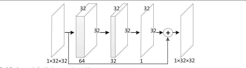
Fig. 1The framework of CSRNet
computational cost and becomes the obstacle for the applications of CS.
In recent years, some deep learning-based methods have been introduced into the low-level problems and get excellent performance, such as image super-resolution [11,12], image artifact removal [13], and CS image recon-struction [14–17]. Recently, some deep network-based algorithms for CS image reconstruction have been pro-posed. ReconNet is proposed in [14], which takes CS measurement of image patch as input and outputs its cor-responding image reconstruction. Especially, for patch-based CS measurement, ReconNet, inspired of SRCNN [11], can retain rich semantic contents at low measure-ment rate as compared to the traditional methods. In [15], a framework is proposed to recover images from CS measurements without the need to divide images into small blocks, but there is no competitive advantage for the performance of the reconstruction compared with other algorithms. In [16, 17], the residual convolutional neural network is introduced in the image reconstruc-tion for compressive sensing, which can preserve some information in previous layers and also can improve the convergence rate and accelerate the training process. Dif-ferent from the optimization-based CS recovery methods, the neural network-based methods often directly learn the inverse mapping from the CS measurement domain to original image domain. As a result, it effectively avoids expensive computation and achieves a promising image reconstruction performance.
In this paper, two different cascaded reconstruction net-works are proposed to meet different sampling methods. Firstly, we propose a compatibly sampling reconstruc-tion network (CSRNet), which is employed to reconstruct high-quality images from compressively sensed measure-ments sampled by a random sampling matrix. In CSRNet, deep reconstruction network module can obtain an ini-tial image with acceptable quality, which can be further improved by residual network module based on convo-lutional neural network. Secondly, in order to improve the sampling efficiency of CS, an automatically sampling module is designed, which has a fully connected layer
to learn a sampling matrix automatically. In addition, the residual reconstruction module is presented, which can match the sampling module. Both the sampling module and its matching residual reconstruction mod-ule form a complete compressive sensing image recon-struction network, named ASRNet. As compared with CSRNet, ASRNet can achieve more than 1 dB gain. The experimental results demonstrate the proposed networks outperform several state-of-the-art iterative reconstruc-tion algorithms and deep-learning-based approaches in objective and subjective quality.
The rest of this paper is organized as follows. In Section2, two novel networks are proposed for different sampling methods. In Section3, the performance of the proposed networks is examined. We conclude the paper in Section4.
2 The methods of proposed networks
In this section, we describe the proposed two networks CSRNet in Fig. 1 and ASRNet in Fig. 4. The first net-work, CSRNet, is designed to reconstruct image from the CS measurement sampled by a random matrix. The sec-ond one is a complete compressive sensing image recon-struction network, ASRNet, consisting of both sampling and reconstruction module. Here, our sampling module contains only one fully-connected layer (FC), which is more powerful to imitate traditional Block-CS sampling process.
Fig. 3The framework of residual reconstruction module
2.1 CSRNet
Our proposed CSRNet consists of three modules, initial reconstruction module, deep reconstruction module, and residual reconstruction module. The initial reconstruc-tion module takes the CS measurement yas input and outputs a B×B-sized preliminary reconstructed image. As shown in the Fig. 1, the deep reconstruction mod-ule takes the preliminary reconstructed image as input and outputs a same-sized image. The deep reconstruc-tion module contains three convolureconstruc-tional layers, shown in Fig.2. The first layer generates 64 feature map with 11×11 kernel. The second layer uses kernel of size 1× 1 and generates 32 feature maps. And the third layer produces one feature map with 7×7 kernel, which is the output of this module. All the convolutional layers have the same stride of 1, without pooling operation, and appropriate zero padding is used to keep the feature map size con-stant in all layers. Each convolutional layer is followed by a ReLU layer except the last convolutional layer. Here, deep reconstruction network module can obtain an ini-tial image with acceptable quality, which is more suitable to residual network module than cascaded residual net-work module [16]. The residual reconstruction network has the similar architecture as the deep reconstruction network, shown in Fig.3, which learns the residual infor-mation between the input data and the ground truth. In our model, we setB=32.
In order to train our CSRNet, we need CS measure-ments corresponding to each of the extracted patches. For a given measurement rate, we construct a measurement matrix,B, by first generating a random Gaussian matrix of appropriate size, followed by orthonormalizing its rows. Then, we applyyi = B×xver−ito obtain the set of CS measurements, wherexver−i is the vectorized version of an image patchxi. Thus, an input-label pair in the training set can be represented as{yi,xi}Ni . The loss function is the average reconstruction error over all the training image blocks, given by
L({W1,W2,W3})= 1 N
N
i=1
f3(f2(f1(yi,W1),W2),W3)−xi2
where N is the total number of image patches in the training dataset, xi is the ith patch, and yi is the corresponding CS measurement. The initial reconstruc-tion mapping, the deep reconstrucreconstruc-tion mapping, and the residual reconstruction mapping are represented asf1,f2, andf3respectively. In addition,{W1,W2,W3}are the net-work parameters which can be obtained in the training.
2.2 ASRNet
Our proposed ASRNet contains three modules, sam-pling module, initial reconstruction module, and residual reconstruction module, as shown in Fig.4. In the sampling
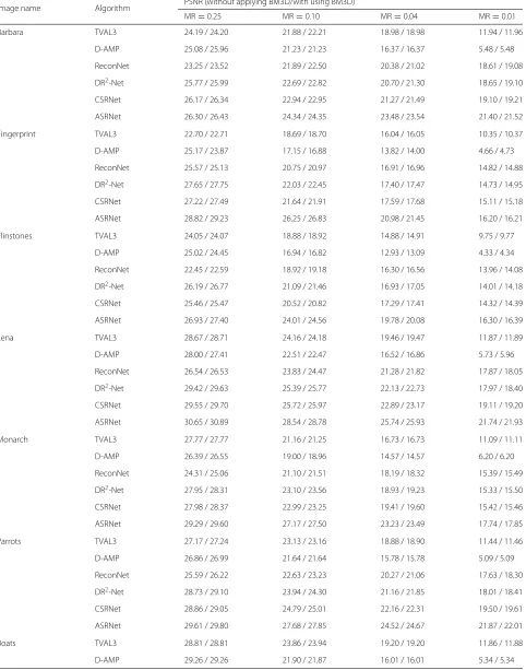
Table 1PSNR valves in dB for testing image by different algorithms at the ratio MR=0.25, 0.1, 0.04, and 0.01
Image name Algorithm PSNR (without applying BM3D/with using BM3D)
MR=0.25 MR=0.10 MR=0.04 MR=0.01
Barbara TVAL3 24.19 / 24.20 21.88 / 22.21 18.98 / 18.98 11.94 / 11.96
D-AMP 25.08 / 25.96 21.23 / 21.23 16.37 / 16.37 5.48 / 5.48
ReconNet 23.25 / 23.52 21.89 / 22.50 20.38 / 21.02 18.61 / 19.08
DR2-Net 25.77 / 25.99 22.69 / 22.82 20.70 / 21.30 18.65 / 19.10
CSRNet 26.17 / 26.34 22.94 / 22.95 21.27 / 21.49 19.10 / 19.21
ASRNet 26.30 / 26.43 24.34 / 24.35 23.48 / 23.54 21.40 / 21.52
Fingerprint TVAL3 22.70 / 22.71 18.69 / 18.70 16.04 / 16.05 10.35 / 10.37
D-AMP 25.17 / 23.87 17.15 / 16.88 13.82 / 14.00 4.66 / 4.73
ReconNet 25.57 / 25.13 20.75 / 20.97 16.91 / 16.96 14.82 / 14.88
DR2-Net 27.65 / 27.75 22.03 / 22.45 17.40 / 17.47 14.73 / 14.95
CSRNet 27.22 / 27.49 21.64 / 21.91 17.59 / 17.68 15.11 / 15.18
ASRNet 28.82 / 29.23 26.25 / 26.83 20.98 / 21.45 16.20 / 16.21
Flinstones TVAL3 24.05 / 24.07 18.88 / 18.92 14.88 / 14.91 9.75 / 9.77
D-AMP 25.02 / 24.45 16.94 / 16.82 12.93 / 13.09 4.33 / 4.34
ReconNet 22.45 / 22.59 18.92 / 19.18 16.30 / 16.56 13.96 / 14.08
DR2-Net 26.19 / 26.77 21.09 / 21.46 16.93 / 17.05 14.01 / 14.18
CSRNet 25.46 / 25.47 20.52 / 20.82 17.29 / 17.41 14.32 / 14.39
ASRNet 26.93 / 27.40 24.01 / 24.56 19.78 / 20.08 16.30 / 16.39
Lena TVAL3 28.67 / 28.71 24.16 / 24.18 19.46 / 19.47 11.87 / 11.89
D-AMP 28.00 / 27.41 22.51 / 22.47 16.52 / 16.86 5.73 / 5.96
ReconNet 26.54 / 26.53 23.83 / 24.47 21.28 / 21.82 17.87 / 18.05
DR2-Net 29.42 / 29.63 25.39 / 25.77 22.13 / 22.73 17.97 / 18.40
CSRNet 29.55 / 29.70 25.72 / 25.97 22.89 / 23.17 19.11 / 19.20
ASRNet 30.65 / 30.89 28.54 / 28.78 25.74 / 25.93 21.74 / 21.93
Monarch TVAL3 27.77 / 27.77 21.16 / 21.25 16.73 / 16.73 11.09 / 11.11
D-AMP 26.39 / 26.55 19.00 / 18.96 14.57 / 14.57 6.20 / 6.20
ReconNet 24.31 / 25.06 21.10 / 21.51 18.19 / 18.32 15.39 / 15.49
DR2-Net 27.95 / 28.31 23.10 / 23.56 18.93 / 19.23 15.33 / 15.50
CSRNet 27.98 / 28.37 22.99 / 23.25 19.41 / 19.60 15.42 / 15.46
ASRNet 29.29 / 29.60 27.17 / 27.50 23.23 / 23.49 17.74 / 17.85
Parrots TVAL3 27.17 / 27.24 23.13 / 23.16 18.88 / 18.90 11.44 / 11.46
D-AMP 26.86 / 26.99 21.64 / 21.64 15.78 / 15.78 5.09 / 5.09
ReconNet 25.59 / 26.22 22.63 / 23.23 20.27 / 21.06 17.63 / 18.30
DR2-Net 28.73 / 29.10 23.94 / 24.30 21.16 / 21.85 18.01 / 18.41
CSRNet 28.86 / 29.05 24.79 / 25.01 22.16 / 22.31 19.50 / 19.61
ASRNet 29.61 / 29.80 27.68 / 27.85 24.52 / 24.67 21.87 / 22.01
Boats TVAL3 28.81 / 28.81 23.86 / 23.94 19.20 / 19.20 11.86 / 11.88
Table 1PSNR valves in dB for testing image by different algorithms at the ratio MR=0.25, 0.1, 0.04, and 0.01 (Continued)
Image name Algorithm PSNR (without applying BM3D/with using BM3D)
MR=0.25 MR=0.10 MR=0.04 MR=0.01
ReconNet 27.30 / 27.35 24.15 / 24.10 21.36 / 21.62 18.49 / 18.83
DR2-Net 30.09 / 30.30 25.58 / 25.90 22.11 / 22.50 18.67 / 18.95
CSRNet 30.14 / 30.36 25.65 / 25.80 22.38 / 22.55 18.99 / 19.09
ASRNet 31.28 / 31.64 28.86 / 29.17 25.52 / 25.72 21.53 / 21.69
Cameraman TVAL3 25.69 / 25.70 21.91 / 21.92 18.30 / 18.33 11.97 / 12.00
D-AMP 24.41 / 24.54 20.35 / 20.35 15.11 / 15.11 5.64 / 5.64
ReconNet 23.15 / 23.59 21.28 / 21.66 19.26 / 19.72 17.11 / 17.49
DR2-Net 25.62 / 25.90 22.46 / 22.74 19.84 / 20.30 17.08 / 17.34
CSRNet 25.85 / 26.15 22.29 / 22.53 20.23 / 20.38 17.75 / 17.90
ASRNet 26.46 / 22.66 25.00 / 25.13 22.74 / 22.88 19.77/ 19.89
Foreman TVAL3 35.42 / 35.54 28.69 / 28.74 20.63 / 20.65 10.97 / 11.01
D-AMP 35.45 / 34.04 25.51 / 25.58 16.27 / 16.78 3.84 / 3.83
ReconNet 29.47 / 30.78 27.09 / 28.59 23.72 / 24.60 20.04 / 20.33
DR2-Net 33.53 / 34.28 29.20 / 30.18 25.34 / 26.33 20.59 / 21.08
CSRNet 34.89 / 35.10 30.96 / 31.35 27.78 / 28.18 23.12 / 23.32
ASRNet 35.85 / 36.19 33.79 / 34.09 30.56 / 30.78 25.77 / 26.14
House TVAL3 32.08 / 32.13 26.29 / 26.32 20.94 / 20.96 11.86 / 11.90
D-AMP 33.64 / 32.68 24.55 / 24.53 16.91 / 17.37 5.00 / 5.02
ReconNet 28.46 / 29.19 26.69 / 26.66 22.58 / 23.18 19.31 / 19.52
DR2-Net 31.83 / 32.52 27.53 / 28.40 23.92 / 24.70 19.61 / 19.99
CSRNet 32.46 / 33.05 28.24 / 28.68 24.55 / 24.85 20.67 / 20.79
ASRNet 33.44 / 33.84 31.47 / 31.87 27.82 / 28.21 23.13 / 23.31
Peppers TVAL3 29.62 / 29.65 22.64 / 22.65 18.21 / 18.22 11.35 / 11.36
D-AMP 29.84 / 28.58 21.39 / 21.37 16.13 / 16.46 5.79 / 5.85
ReconNet 24.77 / 25.16 22.15 / 22.67 19.56 / 20.00 16.82 / 16.96
DR2-Net 28.49 / 29.10 23.73 / 24.28 20.32 / 20.78 16.90 / 17.11
CSRNet 28.58 / 29.19 24.35 / 24.65 21.18 / 21.51 17.61 / 17.67
ASRNet 29.72 / 30.18 27.03 / 27.37 24.03 / 24.32 20.17 / 20.33
Mean PSNR TVAL3 27.84 / 27.87 22.84 / 22.86 18.39 / 18.40 11.31 / 11.34
D-AMP 28.17 / 27.67 21.14 / 21.09 15.49 / 15.67 5.19 / 5.23
ReconNet 25.54 / 25.92 22.68 / 23.23 19.99 / 20.44 17.27 / 17.55
DR2-Net 28.66 / 29.06 24.32 / 24.71 20.80 / 21.29 17.44 / 17.80
CSRNet 28.83 / 29.11 24.55 / 24.81 21.52 / 21.74 18.25 / 18.35
ASRNet 29.85 / 30.17 27.65 / 27.96 24.40 / 24.65 20.51 / 20.66
“MEAN PSNR” is the mean PSNR values among all 11 testing images
module, we use a fully connected layer to imitate the tra-ditional compressed sampling process. And the process of compressed sampling is expressed asyi = Bxiin tradi-tional Block-CS. If the image is divided into B×B blocks, the input of the fully connected layer is aB2×1 vector. For
the sampling ratioα, we can obtainnB=B2×αsampling measurements.
Table 2SSIM valves in dB for testing image by different algorithms at the ratio MR=0.25, 0.1, 0.04, and 0.01
Image name Algorithm SSIM (without applying BM3D)
MR=0.25 MR=0.10 MR=0.04 MR=0.01
Barbara ReconNet 0.6829 0.5732 0.4803 0.3712
DR2-Net 0.7991 0.6364 0.5133 0.3822
CSRNet 0.8024 0.6312 0.5275 0.3957
ASRNet 0.8075 0.7086 0.6213 0.4665
Fingerprint ReconNet 0.9505 0.8026 0.4918 0.1656
DR2-Net 0.9672 0.8576 0.5491 0.1843
CSRNet 0.9635 0.8259 0.5278 0.1802
ASRNet 0.9797 0.9579 0.7938 0.1818
Flinstones ReconNet 0.8553 0.6889 0.4947 0.2758
DR2-Net 0.9279 0.7942 0.5536 0.2959
CSRNet 0.9174 0.7765 0.5743 0.2965
ASRNet 0.9516 0.9262 0.7735 0.4408
Lena ReconNet 0.7784 0.6546 0.5650 0.4390
DR2-Net 0.8540 0.7303 0.6244 0.4529
CSRNet 0.8632 0.7508 0.6471 0.4872
ASRNet 0.8871 0.8398 0.7440 0.5684
Monarch ReconNet 0.7808 0.6494 0.5199 0.3767
DR2-Net 0.8682 0.7401 0.5783 0.3899
CSRNet 0.8691 0.7419 0.5896 0.4032
ASRNet 0.8974 0.8618 0.7506 0.4769
Parrots ReconNet 0.8099 0.7142 0.6315 0.5324
DR2-Net 0.8677 0.7709 0.6741 0.5615
CSRNet 0.8868 0.8032 0.7180 0.6097
ASRNet 0.9019 0.8730 0.7989 0.6790
Boats ReconNet 0.7838 0.6454 0.5277 0.4063
DR2-Net 0.8612 0.7281 0.5876 0.4256
CSRNet 0.8628 0.7198 0.5784 0.4365
ASRNet 0.8842 0.8266 0.6937 0.5054
Cameraman ReconNet 0.7165 0.6193 0.5317 0.4495
DR2-Net 0.7935 0.6872 0.5906 0.4777
CSRNet 0.8043 0.6846 0.6048 0.5053
ASRNet 0.8213 0.7932 0.7014 0.5696
Foreman ReconNet 0.8469 0.7698 0.6802 0.5810
DR2-Net 0.9028 0.8360 0.7506 0.6220
CSRNet 0.9172 0.8598 0.7813 0.6541
ASRNet 0.9280 0.9048 0.8470 0.7247
House ReconNet 0.7832 0.6933 0.6121 0.5286
Table 2SSIM valves in dB for testing image by different algorithms at the ratio MR=0.25, 0.1, 0.04, and 0.01 (Continued)
Image name Algorithm SSIM (without applying BM3D)
MR=0.25 MR=0.10 MR=0.04 MR=0.01
DR2-Net 0.8459 0.7617 0.6753 0.5540
CSRNet 0.8593 0.7785 0.6943 0.5805
ASRNet 0.8751 0.8434 0.7695 0.6296
Peppers ReconNet 0.7488 0.6351 0.5315 0.4222
DR2-Net 0.8232 0.7042 0.5832 0.4365
CSRNet 0.8271 0.7219 0.6195 0.4747
ASRNet 0.8605 0.8386 0.7549 0.5607
Mean SSIM ReconNet 0.7942 0.6769 0.5515 0.4135
DR2-Net 0.8646 0.7497 0.6073 0.4348
CSRNet 0.8703 0.7540 0.6239 0.4567
ASRNet 0.8904 0.8522 0.7499 0.5276
“MEAN SSIM” is the mean SSIM values among all 11 testing images
measurements as input and outputs a B×B-sized pre-liminary reconstructed image. Similar to sampling mod-ule, we also use a fully connected layer to imitate the traditional initial reconstruction process, which can be presented by x˜j = ˜φB× yj. In our design, theφ˜B can be learned automatically instead of computing by the complicated MMSE linear estimation. The residual recon-struction module is similar as the residual reconrecon-struction module in CSRNet, shown in Fig. 3. The output of the residual reconstruction module is the final output of the network.
Given the original image xi , our goal is to obtain the highly compressed measurementyj with the compressed sampling module and then accurately recover it to the original imagexj with reconstruction module. Since the sampling module, the initial reconstruction module, and the residual reconstruction module form an end-to-end network, they can be trained together and do not need to be concerned with what the compressed measure-ment is in training. Therefore, the input and the label are all the image itself for training our ASRNet. Fol-lowing most of deep learning-based image restoration
Table 3Time(in seconds) for reconstruction a single 256×256 image
Models MR=0.25 MR=0.10 MR=0.04 MR=0.01
ReconNet 0.5376 0.5366 0.5415 0.5508
DR2-Net 1.2879 1.2964 1.3263 1.3263
CSRNet 0.5355 0.5375 0.5464 0.5366
Fig. 5The reconstruction results of Parrots at the measurement rate of 0.1 without BM3D.aTVAL3.bDAMP.cReconNet.dDR2-Net.eCSRNet. fASRNet
methods, the mean square error is adopted as the cost function of our network. The optimization objective is represented as
L({W4,W5,W6})= 1 N
N
i=1
f6(f5(f4(xi,W1),W2),W3)−xi2
where{W4,W5,W6}are the network parameters needed to be trained, f4 is the sampling, and f5 and f6 corre-spond the initial reconstruction mapping and residual
reconstruction mapping respectively. It should be noted that we train the compressed sampling network and the reconstruction network together, but they can be used independently.
3 Results and discussion
In this section, we evaluate the performance of the pro-posed methods for CS reconstruction. We will firstly introduce the details during our training and testing.
Fig. 7The reconstruction results of Monarch at the measurement rate of 0.1 without BM3D.aTVAL3.bDAMP.cReconNet.dDR2-Net.eCSRNet. fASRNet
Then, we show the quantitative and qualitative compar-isons with four state-of-the-art methods.
3.1 Training
The dataset used in our training is the set of 91 images in the [14]. The set 5 from [14] constitutes to be our validation set. We only use the luminance component of the images. We uniformly extract patches of size 32×32
from these images with a stride equal 14 for training and 21 for validation to form the training dataset of 22,144 patches and the validation dataset which con-tains 1112 patches. Both CSRNet and ASRNet use the same dataset. We train the proposed networks with different measurement rates (MR) = 0.25, 0.10, 0.04, and 0.01. The Caffe is used to train the proposed model.
Fig. 9The reconstruction results of House at the measurement rate of 0.1 without BM3D.aTVAL3.bDAMP.cReconNet.dDR2-Net.eCSRNet. fASRNet
3.2 Comparison with existing methods
3.2.1 Objective quality comparisons
Our proposed algorithm is compared with four repre-sentative CS recovery methods, TVAL3 [8], D-AMP [5], ReconNet [14], and DR2-Net [16]. The first two belong to traditional optimization-based methods, while the last two are recent network-based methods. For the simu-lated data in our experiments, we evaluate the proposed methods on the same test images as in [14], which con-sists of 11 grayscale images. Here, nine images have size
of 256×256 and two images are 512×512. We compute the PSNR value for total 11 images, and the results are shown in Table1. We use the BM3D [18] as the denoiser to remove the artifacts resulting due to patch processing. It is obvious to see that ASRNet can achieve more than 1 dB gain, as compared with CSRNet. We add SSIM comparison between our proposed networks and network-based methods, ReconNet and DR2-Net, as shown in Table2. From Tables1 and2, it can be found that our proposed CSRNet and ASRNet outperform other
Fig. 11The reconstruction results of Boats at the measurement rate of 0.1 without BM3D.aTVAL3.bDAMP.cReconNet.dDR2-Net.eCSRNet. fASRNet
algorithms under each measurement rates, especially at 0.04 and 0.01. In addition, the performance of our methods decreases slowly compared to other algorithms with the measurement rate down.
3.2.2 Time complexity
The time complexity is a key factor for image compressive sensing. In the progress of reconstruction, the network-based algorithms are much faster than traditional iterative reconstruction methods, so we only compare the time
complexity with ReconNet and DR2-Net. Table3 shows the average time for reconstructing nine sized 256×256 images of those network-based methods.
From the Tables 1, 2, and3, we can observe that the proposed CSRNet and ASRNet outperform the Recon-Net and DR2-Net in terms of PSNR, SSIM, and time complexity. And our ASRNet obtains the best perfor-mance in all objective quality assessments. Notably, ASR-Net run fastest which is very important for real-time applications.
Fig. 13The reconstruction results of Barbara at the measurement rate of 0.25, 0.1, 0.04, and 0.01 without BM3D
Fig. 15The reconstruction results of Flinstones at the measurement rate of 0.25, 0.1, 0.04, and 0.01 without BM3D
3.2.3 Visual quality comparisons
Our proposed algorithm is compared with four rep-resentative CS recovery methods, TVAL3, D-AMP, ReconNet, and DR2-Net in visual. Figures5and6show the visual comparisons of Parrots in the case of measure-ment rate = 0.1 with and without BM3D respectively. It is obvious that the proposed CSRNet and ASRNet are able to reconstruct more details and sharper, which offers better visual reconstruction results than other network-based algorithms. The other three groups are shown in Figs. 7, 8, 9, 10, 11, and 12. The test images under different rates with or without BM3D are shown in the Figs.13,14,15, and16. We can see that our proposed CSRNet and ASRNet outperforms ReconNet and DR2-Net at each measurement rate.
3.3 Evaluation on our proposed architectures
In order to verify the innovation and rationality of our net-works’ architectures in more detail, we add a comparison
Fig. 16The reconstruction results of Flinstones at the measurement rate of 0.25, 0.1, 0.04, and 0.01 with BM3D
express more natural textures and details. All final results outperform previous intermediate results substantially in terms of image quality. It is intuitively confirmed that our proposed networks are reasonable, stable, and reliable.
4 Conclusion
In this paper, two cascaded reconstructed networks are proposed for different CS sampling methods. In most previous works, the sample matrix is a random matrix in CS process. And the first network is a compatibly
sampling reconstruction network (CSRNet), which can reconstruct high-quality image from its compressively sensed measurement sampled by a traditional random matrix. The second network is adaptively sampling recon-struction network (ASRNet), by matching automatically sampling module with corresponding residual reconstruc-tion module. And the sampling module could perfectly solve the problem of sampling efficiency in compres-sive sensing. Experimental results show that the pro-posed networks, CSRNet and ASRNet, have achieved the
Table 4The mean PSNR/SSIM values of 11 test images without applying BM3D
Models MR=0.25 MR=0.20 MR=0.15 MR=0.10 MR=0.04 MR=0.01
CSRNet-i 27.53/0.8322 24.70/0.7554 24.32/0.7405 23.57/0.7068 21.27/0.6085 18.24/0.4401
CSRNet 28.83/0.8703 25.42/0.7847 25.27/0.7818 24.55/0.7540 21.52/0.6239 18.25/0.4567
ASRNet-i 28.48/0.8527 27.39/0.8343 26.81/0.8208 26.76/0.8262 23.89/0.7240 20.37/0.5187
Fig. 17The intermediate and final reconstruction results of CSRNet at the measurement rate 0.20
Fig. 19The intermediate and final reconstruction results of ASRNet at the measurement rate 0.04
significant improvements in reconstruction results over the traditional and neural network-based CS reconstruc-tion algorithms both in terms in quality and time com-plexity. Furthermore, ASRNet can achieve more than 1 dB gain, as compared with CSRNet.
Abbreviations
ASRNet: Adaptively sampling reconstruction network; CS: Compressive sensing; CSRNet: Compatibly sampling reconstruction network
Acknowledgements
The author would like to thank the editors and anonymous reviewers for their valuable comments.
Funding
This work was supported in part by Key Innovation Team of Shanxi 1331 Project (KITSX1331) and Fundamental Research Funds for the Central Universities (2018JBZ001).
Authors’ contributions
YW completed most of the text and implementation of the algorithm. HB and LZ directed this work and contributed to the revisions. YZ reviewed and revised the manuscript. All authors read and approved the final manuscript.
Competing interests
The authors declare that they have no competing interests.
Publisher’s Note
Springer Nature remains neutral with regard to jurisdictional claims in published maps and institutional affiliations.
Received: 2 January 2018 Accepted: 6 August 2018
References
1. D.L. Donoho, Compressed sensing. IEEE Trans. Inf. Theory.52(4), 1289–1306 (2006)
2. G. Lu, Block compressed sensing of natural images. Int. Conf. Digit. Signal Process, 403–406 (2007)
3. J.A. Tropp, Greed is good: algorithmic results for sparse approximation. IEEE Trans. Inf. Theory.50(10), 2231–2242 (2004)
4. D.L. Donohoa, A. Malekib, A. Montanaria, Message-passing algorithms for compressed sensing. Proc. Natl. Acad. Sci. U. S. A.106(45), 18914 (2009) 5. C.A. Metzler, A. Maleki, R.G. Baraniuk, From denoising to compressed
sensing. IEEE Trans. Inf. Theory.62(9), 5117–5144 (2016) 6. Y. Xiao, J. Yang, Alternating algorithms for total variation image
reconstruction from random projections. Inverse Probl. Imaging.6(3), 547–563 (2017)
7. M. Elad, M. Aharon, Image denoising via sparse and redundant representations over learned dictionaries. IEEE Trans. Image Process. 15(12), 3736–3745 (2006)
8. C. Li, W. Yin, H. Jiang, Y. Zhang, An efficient augmented Lagrangian method with applications to total variation minimization. Comput. Optim. Appl.56(3), 507–530 (2013)
9. L. Ma, H. Bai, M. Zhang, Y. Zhao, Edge-based adaptive sampling for image block compressive sensing. Ieice Trans. Fundam. Electron. Commun. Comput. Sci.E99.A(11), 2095–2098 (2016)
10. H. Bai, M. Zhang, M. Liu, A. Wang, Y. Zhao, Depth image coding using entropy-based adaptive measurement allocation. Entropy.16(12), 6590–6601 (2014)
11. C. Dong, C.L. Chen, K. He, X. Tang, Image super-resolution using deep convolutional networks. IEEE Trans. Pattern. Anal. Mach. Intell.38(2), 295–307 (2016)
12. L. Zhao, J. Liang, H. Bai, A. Wang, Y. Zhao, Simultaneously color-depth super-resolution with conditional generative adversarial network. arXiv preprint arXiv:1708.09105. (2017)
13. L. Zhao, J. Liang, H. Bai, A. Wang, Y. Zhao, inIEEE International Conference on Image Processing. Convolutional neural network-based depth image artifact removal (IEEE International Conference on Image Processing, 2017)
14. K. Kulkarni, S. Lohit, P. Turaga, R. Kerviche, A. Ashok, ReconNet: non-iterative reconstruction of images from compressively sensed random measurements. The IEEE Conference on Computer Vision and Pattern Recognition (CVPR) (2016)
15. A. Mousavi, R.G. Baraniuk, Learning to invert: signal recovery via deep convolutional networks. IEEE International Conference on Acoustics, Speech and Signal Processing (2017)
16. H. Yao, F. Dai, D. Zhang, Y. Ma, S. Zhang, DR2-Net: deep residual
reconstruction network for image compressive sensing. The IEEE Conference on Computer Vision and Pattern Recognition (CVPR) (2017) 17. G. Nie, Y. Fu, Y. Zheng, H. Huang, Image restoration from patch-based
compressed sensing measurement. The IEEE Conference on Computer Vision and Pattern Recognition (CVPR) (2017)