R E S E A R C H
Open Access
Cascade of Boolean detector
combinations
Katariina Mahkonen
*, Tuomas Virtanen and Joni Kämäräinen
Abstract
This paper considers a scenario when we have multiple pre-trained detectors for detecting an event and a small dataset for training a combined detection system. We build the combined detector as a Boolean function of thresholded detector scores and implement it as a binary classification cascade. The cascade structure is
computationally efficient by providing the possibility to early termination. For the proposed Boolean combination function, the computational load of classification is reduced whenever the function becomes determinate before all the component detectors have been utilized. We also propose an algorithm, which selects all the needed thresholds for the component detectors within the proposed Boolean combination. We present results on two audio-visual datasets, which prove the efficiency of the proposed combination framework. We achieve state-of-the-art accuracy with substantially reduced computation time in laughter detection task, and our algorithm finds better thresholds for the component detectors within the Boolean combination than the other algorithms found in the literature.
Keywords: Binary classification, Classification cascade, Boolean combination
1 Introduction
Detection and binary classification are fundamental tasks in many intelligent computational systems. They may be considered as the same problem, where an input sample is to be determined into one of two groups, either one of two predefined classes, or as having some property or not. In the field of computer vision, face detection, pedes-trian detection, and car detection are canonical examples that have received a lot of attention [1, 2]. Event detec-tion from audio signal is of wide interest [3]. Detection tasks with multiple measurement modalities available are present, e.g., in biometric identity verification [4] and for medical decisions [5].
For detection of observation from a certain category, i.e., a class, many different types of detectors, trained with dif-ferent data with difdif-ferent statistics—possibly even from different measurement modalities—are often available. Most of the detectors reported in the literature output a score, which denotes the likelihood of the existence of the quested target class, in the input data. A threshold value is then used to provide the classification “target” or “no tar-get” for the input. Thus, a threshold value may be used to
*Correspondence:[email protected]
Tampere University of Technology, Korkeakoulunkatu 1, 33720 Tampere, Finland
control the false negative-false positive trade-off, i.e., an operating point of the detector.
The different detectors may have very different per-formance, and the scores given by them are not fully correlated. Therefore, the combination of their outputs provides an opportunity to obtain a combined detector with performance superior to any of the components.
The cost of classification in terms of time and compu-tational power, besides accuracy, is an important factor in many detection problems. Some of the detectors are very fast to execute while others are computationally heavy. An effective way to reduce the cost of classification is to use a sequential decision making process which asks for new resources only if needed for required accuracy.
We propose a new method for combining multiple sen-sitivity tunable detectors, i.e., detectors which output like-lihood scores, to form a computationally efficient binary classification cascade. The component detectors are not restricted to be based on a single feature set, but may even operate on different measurement modalities. They have preferably been trained with different datasets to introduce uncorrelatedness in their output scores. For
combining the available sensitivity tunable detectors, we propose to utilize a monotone Boolean function built usingAND (∧) and OR(∨) operators in disjunctive nor-mal form (DNF). A Boolean function (BF) is said to be monotone, if changing the value of any of the input vari-ables from 0 to 1 cannot decrease the value of the function from 1 to 0. For continuous data binarization, we use sim-ilar procedure as presented in [6]. Thus, a monotone BF on this data performs a monotone partition of the space of measurement values.
A BF lends itself naturally to sequential evaluation, which is an integral property of a decision process of a classification cascade. Also, by utilizing a BF of thresh-olded detector scores, we avoid inferring class probabil-ities from the scores, which would be error prone while having only a small dataset for combined system train-ing. In the proposed OR of ANDs function (BOA), each
detector score is compared to multiple threshold levels, which allows formulating any monotonic decision bound-ary while making the classification decision in a computa-tionally efficient way. The BOA cascade detector itself is trained to be sensitivity controllable as well.
The contributions of the paper are (1) a monotone BooleanORofANDs (BOA) binary classification function to build a cascaded combination of multiple sensitivity tunable detectors, (2) an algorithm to train a BOA com-bination, and (3) utilizing a cascaded decision making process for audio-visual detection task.
For evaluating the proposed BOA detector cascade and the training algorithm to set its parameters, we use two audiovisual databases for two detection tasks, namely MAHNOB laughter dataset [7] for laughter detection task and CASA dataset [8] for video context change detec-tion task. In the laughter detecdetec-tion task, we show that the accuracy of detection with a BOA cascade is superior to the other detection accuracies reported in the literature, while the computation time of detection is remarkably reduced compared to the other solutions. With three com-ponent detectors for the video context change detection, we show that the proposed BOA training algorithm out-performs alternative Boolean combination training algo-rithms found in the literature.
In the following section, we introduce the work related to Boolean detector combinations and algorithms for training Boolean combination parameters, as well as the work on cascaded detectors presented in the literature. The proposed Boolean OR of ANDs combination, and the algorithm to set its parameters are presented in Section3. The experimental setup and the results obtained are pre-sented in Section4.
2 Related work
This paper proposes combining multiple tunable detec-tors robustly utilizing a monotone DNF-BF, named BOA,
the evaluation of which is formulated as a computationally efficient classification cascade. Thus, we first review the literature on Boolean detector combinations and BFs in general. Then, we review the algorithms suitable for train-ing a Boolean combination. Finally, we discuss the litera-ture on classification cascades.
2.1 Boolean detector combinations
Using a Boolean conjunction or a Boolean disjunction for combining multiple detectors has been proposed in several studies, for example in [9–11]. Sensitivity tunable detector functionsfm : x → Rform=1. . .Mare uti-lized within a combination. Each detector functionfm(x) produces a scorelm, which denotes likelihood of the target appearing in the samplex. The Boolean conjunction ofM sensitivity tunable detectors is
B(x;θ)= M
m=1
fm(x)≥θmAND
, (1)
and the Boolean disjunction is
B(x;θ)= M
m=1
fm(x)≥θmOR
, (2)
where θ denotes all the thresholds θm∗ used within the combination. All of the studies [9–11] report that either a conjunctive or a disjunctive Boolean combi-nation of detectors do improve the detection accuracy over component detectors, provided that the thresholds
θ∗
1,θ2∗,. . .,θM∗are set appropriately.
Mixtures of AND and OR operators within a Boolean
combination have been investigated in [12]. Utilizing notation, where the detector functionfm(x)identifiersm are listed in vectors zq, q = 1. . .Q, eachzq containing
Mq identifiers, this kind of Boolean OR of ANDs
combination is
B(x;θ)= Q
q=1 ⎡ ⎣
Mq
i=1
fzq(i)(x)≥θzq(i) ⎤⎦
. (3)
As a big limitation of (3) proposed in [12], compared to the BOA combination that we suggest, is that only one thresholdθmfor each target likelihood scorefm(x)=lmis allowed.
In addition to AND and OR operators, the Boolean
negation, (NOT), and as a consequence also the exlusive-OR (XOR) are utilized in the detector combinations in
Boolean detector combinations where each of the avail-able target likelihood scoresfm(x) = lm, m = 1. . .M may be cast to Boolean values using multiple thresholds
θ1
m, θm2,. . . are first made use of in [14]. However, the space of the Boolean combinations generated by their algorithm is left unspecified.
A question of how to select the best performing Boolean combination for a certain problem, while havingM sen-sitivity tunable detectors, has been posed in many of the abovementioned works. To select between conjunc-tive (1) and disjunctive (2) combinations, in [10, 16], it is suggested to investigate the class-conditional cross-correlations of detector scores and to consider whether the specificity or the sensitivity is more important. The conjunctive fusion rule (1), which emphasizes specificity, should be used if there is negative correlation between detector outputs for samples of the “non-target” class. If on the other hand the correlation of detector output scores for samples from the “target” class is weak, disjunc-tive fusion rule (2) emphasizing sensitivity should be used. All in all, a Boolean combination is able to exploit negative or weak correlation of detector scores.
To select among the combinations of the form (3), rules of thumb have been drawn in [12] according to average cross-correlations between the scores from the used detectors. It is shown for three detectors with Gaussian score distributions and identical pairwise cross-correlations that either a conjunctive combination (1), a disjunctive combination (2), or a type (3) combination
B(x;θ)= f1(x)≥θ1vote
∧f2(x)≥θ2vote ∨ f1(x)≥θ1vote
∧f3(x)≥θ3vote ∨ f2(x)≥θ2vote
∧f3(x)≥θ3vote ,
which stands for a majority vote rule, is the best and out-performs the component detectors. The one of those to be selected depends on class conditional cross-correlations between detectors.
The Iterative Boolean Combination (IBC) method in [14] is specifically designed to find the best possible Boolean combination, not restricted to monotone func-tions, for a certain sensitivity level of a combination. The search space of BFs is nevertheless restricted to avoid an unfeasibly large number of possibilities. The IBC method results in variety of Boolean detector compounds, but the study does not provide analysis of the form of the gen-erated compounds nor characteristics of their resulting decision boundaries.
Theory of constructing BFs of unrestricted form, specif-ically in DNF as well as in CNF (conjunctive normal form), has been studied in depth, e.g., in [17]. BFs for classifica-tion have been studied vastly under terms logical analysis and inductive inference. Logical Analysis of Data (LAD)
[18,19] is a combinatorics- and optimization-based data analysis method first introduced in [20]. LAD methodol-ogy focuses on finding DNF-BF-type representations for classes.
The term inductive inference is used in many early texts concerning topics of machine learning, many of those discussing Boolean decision-making, e.g., [21,22]. Using data binarization, e.g., as proposed in [6], all these results concerning BFs may be utilized in conjunction with continuous valued data.
Any BF may be converted into a binary decision tree, while the structure of the tree is generally not unique. In case of the proposed BOA DNF-BF, the
correspond-ing deterministic read-once binary tree has depth ≥
log2(Nθ+1). In maximally deep node arrangement, the tree becomes a single branch tree with depth equal to the numberNθ of thresholds used in the BOA function. However, this kind of binary tree representation does not highlight the computational advantages of BOA cascade that we are interested in.
2.2 Algorithms for training a Boolean combination
The parameter θ of a Boolean combination function
B(x;θ)denotes all the thresholdsθmn ∈θ form=1. . .M, n=1. . .Nmused in the combination. For a Boolean com-bination B(x;θ) to perform well, suitable values for the set θ of thresholds must be found. Most of the studies rely on training data-based exhaustive search for select-ing the threshold values for θ, e.g., [10, 12, 13]. The computational load of this approach is OT|θ|, where |θ| = M
m=1Nm is the total number of thresholds in θ andT is the number of threshold values tested for each detector. The exhaustive search becomes computationally prohibitive if there are more than a couple of threshold values to find. Thus, more efficient algorithms are needed. In addition to algorithms readily proposed for tunable classification function training, we shortly review algo-rithms which have been developed for BF training for one operating point and their extensions to incremental learning.
A fast method for finding setsθ of thresholds for differ-ent sensitivity levels of a Boolean combinationB(x;θ)is presented in [10]. The method exploits the receiver oper-ating characteristic (ROC) curve of each utilized detector dm(x,θ) =
fm(x)≥θ
. The ROC curve shows the true positive rate (tpr) against the false positive rate (fpr) at every operating point, defined by the thresholdθ, of the detector. When θ = −∞, the classification by d(x,θ)
results intpr = 100% and fpr = 100%. On the other
hand, when θ = +∞, then tpr = fpr = 0. The
disjunctive combination of detectorsdAanddB,dA=dB, are provided as
tpr∧fpr∧= max
fprA·fprB=fpr∧
tprA(fprA)·tprB(fprB)
(4)
and
tpr∨fpr∨=
max fprA+fprB−fprA·fprB=fpr∨
tprA(fprA)+tprB(fprB)−tprA(fprA)·tprB(fprB)
,
(5)
wheretpr∗(fpr∗)denotes the true positive rate of a detec-tord∗(x;θ)at an operating pointθ where its false positive rate isfpr∗.
The efficiency of the method is based on an assump-tion that the classificaassump-tions made by different detectors are independent. Unfortunately, this often does not hold in practice. If the same measurement set or the same set of features are used for multiple detectors, or if multiple thresholds are to be found for a certain target likelihood lmwithin a Boolean combination, dependencies between classifications are very likely. We compare our algorithm to this Boolean algebra of ROC curves in the Section 4
and use an implementation for BOA training shown in Appendix1.
Another algorithm that does not assume independence of the used detectors was proposed in [11]. It suggests training the combination iteratively by finding thresholds for two detectors or partial combinations at a time, sim-ilarly to the Boolean algebra of ROC curves presented above. In this approach, the search of the best thresh-olds for a Boolean combination is done via exhaustive search over all the possible threshold settings for the two systems to be merged. In the ROC space, with all the pos-sible threshold settings, a Boolean combination produces a constellation of performance points. The left top edge of this constellation, consisting of the operating points of superior performance, was introduced by [23] as the con-vex hull of the ROC constellation. In the algorithm of [11], before each new component fusion, the set of possible threshold values for the newly built partial combination is pruned to constitute of only the thresholds correspond-ing the performance points at the convex hull of this ROC constellation. The algorithm is originally designed for pure conjunctive (1) or disjunctive (2) Boolean combi-nations, but we have implemented it to deal with a BOA as described in the Appendix1, and we use it for comparison to our algorithm.
In the literature concerning BFs, there are many algo-rithms, which are designed to find a BF which perfectly classifies the training data X0,X1 in {0, 1}Nattr. Find-ing the simplest possible BF to explain some data is an NP complete optimization problem with 22Nattr
possible solutions. Some of the algorithms are designed assuming
monotonicity of data, the assumption which diminishes the number of possible solutions remarkably [24]. The number of possible BFs is further reduced in the case of continuous data which is binarized as in [6]. In this case, the data withM Nattrcontinuous attributes actually resides in theM-dimensional manifold of theNattr dimen-sional space of binarized data. However, the number of possible BFs is still exponential. A few of the approaches target finding a BFn with imperfect classification perfor-mance, which usually is the desirable learning result with imperfect data.
Because of NP completeness of finding the best BF to explain some data, most of the algorithms in the lit-erature operate in iterative manner using some greedy heuristics. An Aq algorithm [25] and LAD [20]-based methods construct a DNF-BF via iteratively searching for good conjunctions, each of which covers a part of pos-itive training samples, to be combined disjunctively. On the contrary, OCAT-RA1 -algorithm [26], based on idea of one-clause-at-a-time (OCAT) [27], builds a CNF-BF via iterative selection of disjunctions. In case of continuous data binarized as in [6], algorithms developed for decision tree learning, e.g., ID3 [28], C4.5 [29], CART [30] are also suitable for DNF-BF building.
TheAqalgorithm and LAD-based methods are to find two DNF-BFs which provide perfect classification of the training data. One function is to be used for detection of the positive class, and the other one for detecting the negative class. The covers, i.e., subspaces for which BF = true, of these DNF-BFs are disjoint, leaving part of the input space uncovered by either function. The algorithms use different heuristic criteria when searching for suitable conjunctions, i.e.complexesin terms ofAq.
For Aq algorithm the user may choose the criterion, one possible choice beings the number of positive sam-ples covered by the complex, that is, conjunction. For LAD methodology, different criteria for optimality of con-junctions, calledpatternsin LAD, are discussed in [31]. Selectivity criterion favors minterms based on data, and evidential criterion favors patterns covering as many data samples as possible. Algorithms for constructing pat-terns according to these different criteria are given in [18,32,33].
iteratively selecting attributes for it based on their rank of Ntp(a)/Nfp(a), whereNtp(a)(Nfp(a)) is the number of positive (negative) training samples, which have attribute a = 1. New attributes are selected until all the positive samples are covered by their disjunction.
The binary tree building algorithms, which iteratively build the tree by starting from the root node and per-forming a new split at every iteration, implicitly facilitate different level generalizations of data and generate a deci-sion function of DNF-BF form. The splitting criterion for selecting attributes for new nodes in ID3, C4.5, and C5.0 is gain in information entropy. ID3 is applicable with bina-rized data, while C4.5 and C5.0 can handle continuous data by implicitly performing the binarization by usage of thresholds. The CART algorithm uses either Gini impu-rity or Twoing criterion to decide about the attributes used in nodes of the tree.
Incremental learning algorithms enable updating a clas-sification function when new data becomes available. Some of the algorithms keep all the data available for future updates, while some algorithms discard the orig-inal data and perform the update based on new data only. Incremental algorithms, which utilize all the original training data aside of some new data, for updating a BF are for example GEM [35] and IOCAT [36].
Both of the algorithms assume a DNF-BF, and their update procedures consist of two phases. At the first phase, if some of the new negative samples are misclas-sified by the original DNF-BF, the faulty conjunctions are located and specialized to not to cover those new samples. Both of the algorithms perform this step by replacing each faulty conjunction by new conjunctions which are trained using data inside the cover of the orig-inal conjunction. GEM utilizesAqalgorithm and IOCAT utilizes OCAT-RA1 algorithm for this re-training. At the second phase of BF update, the DNF-BF is updated in terms of the uncovered new positive samples. GEM generalizes the existing conjunctions to cover the new positives usingAq.
In IOCAT, for each uncovered new positive sample, a conjunction, i.e.,clausein terms of IOCAT, to be gener-alized is selected based on ratioNtp(clause)/Nattr(clause) of the number of positive samples covered by the clause Ntp(clause) and the number of attributes in the clause Nattr(clause). The selected conjunction is then retrained with non-incremental OCAT-RA1 algorithm using all the negative samples, the new positive sample and the pos-itive samples within the space covered by the selected conjunction.
2.3 Cascade processing for reduced computational load of classification
The goal in cascaded processing for detection is in reduc-ing the computational cost of classification. The idea is
to evaluate the input in stages, such that at each cas-cade stage new information about the input is acquired and then either the classification is released or the next cascade stage is entered for new information. Decision cascades have been investigated mostly in the field of machine vision starting from [37,38]. Face detection and pedestrian detection are the most common application areas where decision cascades have been used, e.g., in [39–42]. Decision cascades have been utilized in other fields, e.g., in [43] for cancer survival prediction and in [44] for web search.
In the task of object detection from images, the heavily imbalanced class distribution, as most of the search windows of different sizes and positions do not contain the target object, offers great possibilities to make “non-target” classification with minor examina-tion. Object detection cascades are designed such that gradually more and more features are extracted for increased classification certainty. A class estimate is released as soon as the classification certainty is high enough. If this is the case before all the obtainable features or measurements have been extracted, computational savings appear.
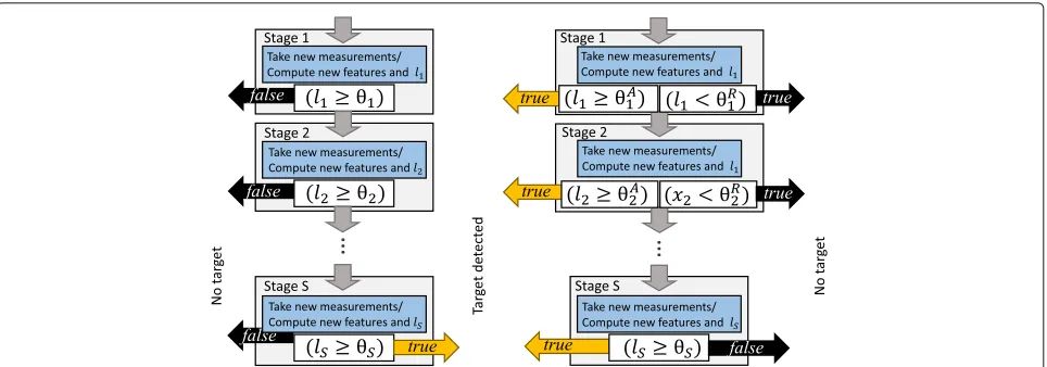
The first generation object detection cascades, used for example in [38], are able to make early classification to the “non-target” class only, as illustrated in Fig.1(left). To classify the input into the “target” class, the input must pass all testsfs(x)≥θs
of the cascade stagess=1. . .S. This kind of one-sided cascade performs a conjunctive Boolean combination function
B(x;θ)= S
s=1
fs(x)≥θs
.
The solutionB(x;θ) = truedenotes classification to the “target” class, andB(x;θ)=falsedenotes classification to the “non-target” class.
The second generation object detection cascades intro-duced in [45] and used also in [46] are able to make the early classification to both the classes, as illustrated in Fig.1(right). They utilize two thresholds on the tar-get likelihood score fs(x) = ls at each cascade stage s = 1. . .S− 1. One threshold,θsreject, is used for early rejection, i.e., early classification to “non-target” class, if fs(x) < θsreject
= true. Another threshold, θsaccept, is used for early detection if fs(x)≥θsaccept
Fig. 1Two types of binary classification cascades. Typical object detection cascades utilized in computer vision. Left: an asymmetrical type cascade for classifying efficiently the “non-target” windows. Right: a symmetrical detection cascade which is capable of early classification to both classes
B(x;θ)= S
s=1 s−1
m=1
fm(x)≥θmreject
∧fs(x)≥θsaccept
,
(6)
whose outputB(x;θ)= truedenotes the classification to the “target” class andB(x;θ)=falsedenotes classification to the “non-target” class.
A cascade may be seen as a one branch decision tree, if the notion of tree is broadened from the traditional def-inition that a node makes a decision based on only one input attribute. In a “cascade-tree,” a node function may utilize multiple input attributes, and the function may partition the corresponding input space freely to assign inputs to any of the leaves, i.e., classes, or down the branch to the next level node (stage of the cascade). In a cascade, the order of attribute acquisition is fixed in con-trast to input-dependent order of attribute usage with a traditional decision tree.
For training, a detection cascade for computer vision applications, where the detectors to be utilized are designed having close to infinite pool of image features, e.g., Haar, HoG, an efficient cascade structure is guaran-teed by concurrent design of detector functions fs,s = 1. . .S, their thresholds θs∗ and the cascade length S as proposed in [40, 47]. For a cascade with fixed length S, a method for concurrent learning of object detectors and their operating points is proposed in [39]. The methods proposed in the literature for finding operating points for pre-trained detectors within a detection cascade mostly assume strong correlation among detector scores. This is the case in [48], where an object detection cascade is designed using cumulative classifier scores, as well as in [45,46], where the proposed algorithms are based on the assumption that the detector scores are highly pos-itively correlated. If the detector scores are negatively
or not correlated, those cascade training strategies turn unsuitable.
3 Methods
For combining multiple detector functions fm(x) = lm, m=1. . .M, which output likelihood scoresl1,l2,. . .,lM for the same target class, we propose to use a a BF. The proposed combination function utilizes BooleanAND(∧) andOR(∨) operators and it is defined in disjunctive
nor-mal form. The proposed Boolean OR of ANDs function
(BOA) B yields a Boolean output B :x→ {false, true}. The BOA output B(x)=truedenotes inputxclassification to the “target” class and the BOA output B(x) = false, i.e., ¬B(x) = true, denotes classification to the “non-target” class.
Generally, a BF—possibly infinite—over a combina-tion of thresholded detector scores is capable of
pro-ducing any binary partition of the input space x or
the space of target likelihood scores (l1,l2,. . .,lM).
Due to exclusion of the Boolean NOT rule, a BOA
combination restricts the space of different partitions such that the spaces (l1,l2,. . .,lM) |B(x)=false
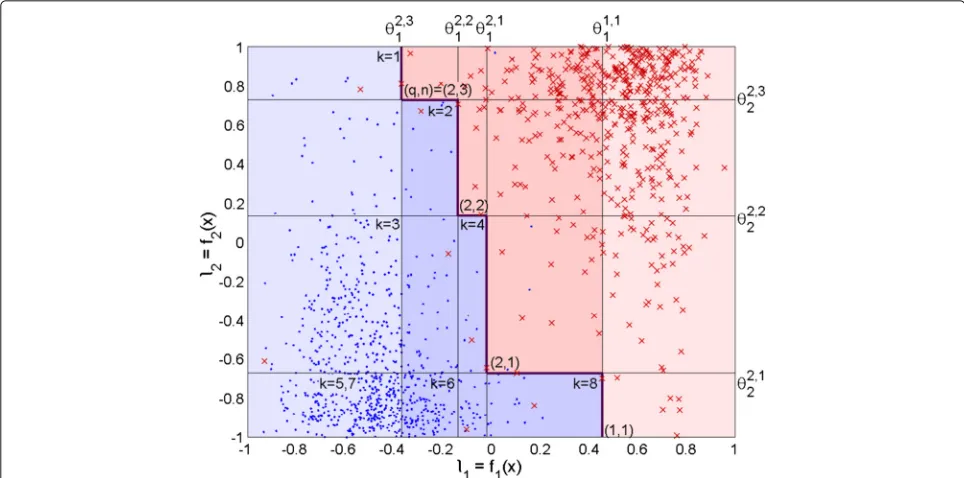
and {(l1,l2,. . .,lM) | B(x)=true}are simply connected and the decision boundary is monotonic. This is illustrated in the example of Fig.2, where the data points indicate laugh-ter likelihoods from videos of MAHNOB laughlaugh-ter dataset [7], which is used in our evaluations.
We build a BOA combination of detector functions fm(x) = lm, m=1. . .Musing BooleanOR(∨) andAND
(∧) operators as
B(x;θ)= Q
q=1 Nq
n=1 ⎡ ⎣Mq
i=1
fzq(i)(x)≥θ q,n zq(i)
⎤
⎦, (7)
Fig. 2Example of BOA decision boundary. Illustration of classification of MAHNOB Laughter dataset videos with BOA. Datax∈X= {X0,X1}from
two classes, “laughter” and “speech,” is represented in terms of two target likelihood scoresl1andl2. The data samples from the “laughter” classX1
are shown with red crosses and the data samples of the “speech” classX0are shown with blue dots. The resulting decision boundary by the BOA
combination (10) is shown with the bold angular line. Each thresholdθmq,n,m=1, 2,q=1, 2,n=1, 2, 3 is illustrated with a thin line. The space of
target likelihood scores where B(x;θ)=trueis colored with pink background, and the space where¬B(x;θ)=trueis colored with blue background. The palest background colors illustrate the subspaces, where the decision is done using the scorel1only
term Mi=q1
lzq(i)≥θ q,n zq(i)
in (7) is aconjunction over the Boolean threshold comparisons of the target likeli-hood scores {lm| ∃i m = zq(i)}. The multiplicity of a conjunction typezqis denoted byNq.
Every conjunction, enumerated by(q,n), operates with a distinct set of thresholdsθzq,nq(i), i=1. . .Mq.
The negation of the BOA function (7) is used for the cascade implementation of its evaluation. In the BOA cas-cade, the classification to the “non-target” class is formu-lated via the negation of the BOA function—whenever the negated BOA function equalstrue. The Boolean negation of B(x;θ)in (7), in disjunctive normal form, is
¬B(x;θ) = K
k=1 ⎡
⎣ Q
q=1 Nq
n=1
fzq(I(k,q,n))(x) < θ q,n zq(I(k,q,n))
⎤
⎦
= M1
i1,1=1 M1
i1,2=1 M1
i1,3=1 · · ·
M1
i1,N1=1
N1-operators , i.e.,MN11conjunctions M2
i2,1=1 M2
i2,2=1 · · ·
M2
i2,N2=1
N2-operators, i.e.,MN22conjunctions · · ·
· · · MQ
iQ,1=1 MQ
iQ,2=1 · · ·
MQ
iQ,NQ=1
NQ
-operators, i.e.,MNQQ conjunctions ⎡
⎣ Q
q=1 Nq
n=1
fzq(iq,n)(x) < θ q,n zq(iq,n)
⎤
⎦.
where the number of conjunctions is given by K =
Q
q=1M Nq
q , and the indexI(k,q,n)of the detector func-tion identifiermwithin vectorzqof the first representa-tion is given by
I(k,q,n)= ⎢ ⎢ ⎢ ⎢ ⎢ ⎢ ⎣ ⎢ ⎢ ⎢
⎣Qk−1 i=q+1MNi i
⎥ ⎥ ⎥ ⎦
MqNq−n ⎥ ⎥ ⎥ ⎥ ⎥ ⎥
⎦modMq +1, (9)
Figure2illustrates the decision boundary using a BOA combination withz1=[1] ,z2=[1, 2], andN1=1,N2=3, which is
B(x;θ)=l1≥θ11,1
∨ 3
n=1
l1≥θ12,n
∧ l2≥θ22,n
(10)
and its negation is
¬B(x;θ)=
8
k=1
⎡ ⎣2
q=1 Nq
n=1
fzq(I(k,q,n))(x) < θ q,n zq(I(k,q,n))
⎤ ⎦
=
2
i1=1 2
i2=1 2
i3=1
⎡
⎣f1(x)<θ11,1∧
Nq
n=1
fzq(in)(x)<θzqq,n(in)
⎤ ⎦
= l1< θ11,1∧l1< θ12,1∧l1< θ12,2∧l1< θ12,3
∨l1< θ11,1∧l1< θ12,1∧l1< θ12,2∧l2< θ22,3
∨l1< θ11,1∧l1< θ12,1∧l2< θ22,2∧l1< θ12,3
∨l1< θ11,1∧l1< θ12,1∧l2< θ22,2∧l2< θ22,3
∨l1< θ11,1∧l2< θ22,1∧l1< θ12,2∧l1< θ12,3
∨l1< θ11,1∧l2< θ22,1∧l1< θ12,2∧l2< θ22,3
∨l1< θ11,1∧l2< θ22,1∧l2< θ22,2∧l1< θ12,3
∨l1< θ11,1∧l2< θ22,1∧l2< θ22,2∧l2< θ22,3. (11)
The corners of the resulting decision boundary are formed by the conjunctions (q,n) = (1, 1), (2, 1),(2, 2), and(2, 3)of (10), which are designated in Fig.2by the con-junction indexes(q,n) next to each corresponding outer corner of space { (l1,l2) | B(x;θ) = true }. The outer corners of space { (l1,l2) | ¬B(x;θ) = true }, which are generated by the conjunctionsk = 1. . .8 of (11), are similarly designated in Fig.2.
There may be redundancy in the BOA equation or its negation, depending on values of the
thresh-olds selected for θ. A conjunction within a BOA
is redundant, if the BOA decision boundary does
not change by removing that conjunction from the BOA equation.
Considering a BOA with conjunction listsz1,z2,. . .,zQ and conjunction multiplicities N1,N2,. . .,NQ, to find out whether a conjunction (q,nq) is redundant or not, its thresholds θzq,nq
q(i)|i=1. . .Mq
must be examined.
Each threshold θzq,nq
q(i) must be compared to thresholds θp,np
zp(j), zq(i) = zp(j) = m, on the same target likelihood score lm, which are used within other conjunctions
p,np
of the BOA. The conjunctions p,np
to be considered are those with zp containing m = zq(i) and possibly other identifiers from zq. The list zp may not contain identifiers not listed in zq. Formally,
zp|p=qand ∃i,jm=zp(j)=zq(i)and∀i∈1. . .Mp ∃j zp(i)=zq(j). The range ofnpfor(p,np)is naturally np = 1. . .Np. For a conjunction (q,nq) to be non-redundant, one of its thresholdsθzq,nq
q(i), i=1. . .Mqmust be smaller than any thresholdθzp,np
p(j),zq(i)=zp(j)=m, in its corresponding conjunctions p,np. That is, in conjunc-tion(q,nq)there must exist at least one thresholdθmq,nqfor whichθmq,nq < θmp,npof all the corresponding conjunctions
p,np
.
3.1 BOA as a binary classification cascade
Algorithmically, a BF is evaluated in steps, i.e., sequen-tially. If any of the conjunctions of BOA function (7) or its negation (8) resolves astrue, the entire functions (7) and (8) become determinate. In other words, as soon as any of the conjunctions(q,n), q=1. . .Q,n=1. . .Nqof a BOA B(x;θ)outputstrue, i.e., Mi=q1
lzq(i)≥θ q,n zq(i)
= true, it means that B(x;θ) = true. Without evaluating the rest of the BOA conjunctions the detection result “target event detected” may then be announced. Sim-ilarly, if any of the conjunctions k = 1. . .K of the negation of the BOA ¬B(x;θ) outputs “true,” that is, if
Q
q=1
Nq
n=1
lzq(I(k,n,q))< θ q,n zq(I(k,n,q))
=true, it means that¬B(x;θ)=true. The evaluation can then be stopped and the classification result “non-target” can be released.
Computationally, the heaviest part of BOA evaluation is the acquisition of target likelihood scoreslmfor an input samplex by computing the functionsfm(x) = lm, m= 1. . .M. The cost of threshold comparisons within BOA may be considered negligible. From computational aspect of evaluating a BOA, once the likelihood score lm is acquired, all the Boolean comparisons (lm ≥ θm∗) and
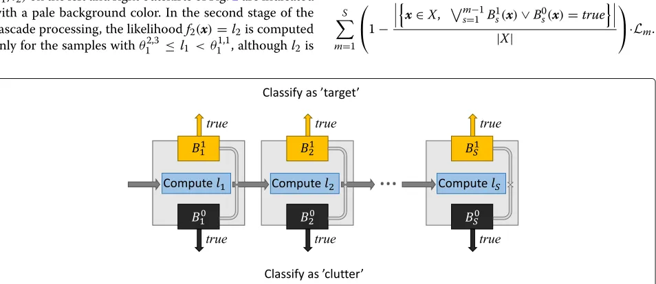
We have implemented the BOA as a binary classifica-tion cascade, where a cascade stages∈ {1. . .S}calculates a score fm(x) = lm = ls using a predefined detector functionfmand offers a possibility for releasing the clas-sification result, as shown in Fig.3. Internal decisions at each stages=1, 2,. . .,Sof the BOA cascade, whether to release a class estimate or to enter the next cascade stage, are made with BFsBclasss ((l1,l2,. . .,ls)), s = 1. . .S, i.e. B11(l1),B01(l1),B12(l1,l2),B02(l1,l2),. . . ,B1S(l1,l2,. . .,lS)and B1S(l1,l2,. . .,lS). That is, the functionsB1s andB0s of cas-cade stagesutilize the target likelihood scoresl1,l2,. . .,ls. All these functions are partitions of the BOA function B(x;θ)of (7) and its negation¬B(x;θ)of (8) such that
B(x;θ)=B11∨B12∨. . .∨B1S (12)
and
¬B(x;θ)=B01∨B02∨. . .∨B0S. (13)
Formal expressions for the partition of the BOA function (7) into functionsB11,B21,. . ..,B1Sand the BOA negation (8) into functionsB01,B02,. . ..,B0Sare derived in Appendix2.
As an example, operation process of BOA cascade B(x;θ)=l1≥θ11,1
∨3
n=1 l1≥θ12,n
∧l2≥θ22,n for MAHNOB laughter data classification is illustrated in the Fig. 2 with the background color of the l1 -vs. l2-axis and is as follows. The classification takes place at the first cascade stage for all the samples x for whom B11(x) =
l1≥θ11,1
= true or B01(x) =
l1<min
θ2,1
1 ,θ12,2,θ12,3
= l1< θ12,3
= true. In the first case, the classification is “Laughter detected,” and in the second case “No Laughter.” These subspaces of
(l1,l2)on the left and right outskirts of Fig.2are indicated with a pale background color. In the second stage of the cascade processing, the likelihoodf2(x)=l2is computed only for the samples withθ12,3 ≤ l1 < θ11,1, althoughl2is
shown for all the samples in the Fig.2. With the dataset in the Fig.2, it means that classification of approximately 65% of the samples are made using the detector function f1only.
The computational efficiency of the cascade naturally depends on the order of detector methods to be utilized at cascade stages. Generally, the faster methods should be evaluated first, and the slower ones later. If the methods fm, m=1. . .Mhave very different computational loads
Lm, m=1. . .M, it is very likely that a cascade ordered such thatLs Ls+1,s=1. . .S−1 is the most efficient one. Precisely, the most computationally efficient cascade structure may be defined via local inequalities among each two consecutive stagessands+1 as follows. If we denote the probability of a sample arriving stagesto be classified at stagesafter computingls=fs(x)withP1, and the prob-ability of a sample arriving stagesto be classified at stages if the detector methodfs+1would be utilized instead of the methodfswithP2, it must hold thatP1≥(Ls/Ls+1)P2.
In our work, the computational loads of the detec-tor methods are very different from each other, i.e.
Ls/Ls+1 1. Thus within the BOA cascade the detec-tor methodsfmm=1. . .Mare ordered according to their computational loads. For notational simplicity we assume that the detector methodsfmused in a BOA cascade are enumerated such that for their computational loads Lm it holds that Lm Lm+1, and now in a BOA cascade fs = fm. The Table 3 demonstrates the computational efficiency achieved in our experiments.
For a sample in a datasetX, the computational load of classification with a BOA cascade is on average
S
m=1 ⎛ ⎝1−
!!
!x∈X, ms=−11Bs1(x)∨B0s(x)=true!!! |X|
⎞ ⎠·Lm.
Fig. 3BOA cascade. Classification process with BOA classification cascade. At each stagesof the cascade new target likelihood scorefs(x)=lsis
computed and either classification is made, or next stage is entered. The internal Boolean decision makersB1
1,B12, . . . ,B1Sare partitions of BOA
function (7), andB0
To design a specific type of BOA cascade, e.g., one-sided or symmetrical, the lists zq,q = 1. . .Q, which determine the detector functions to be utilized within the conjunctions of the BOA, must be selected appropri-ately. For data with clearly unbalanced class distribution, one-sided cascade is computationally efficient if the early classification option is available for the prevalent class. This is the case if the decision-makers Bprevalents ,s = q. . .S for the prevalent class are functioning while the decision-makers Brares ,s = 1. . .S −1 for the rare class are null/nonexistent as Brares (x) = false ∀ x. Thus, for the usual case, where the “target” class is rare and the “non-target” class is the prevalent one, to ensure a compu-tationally efficient one-sided BOA cascade, the BOA must be conjunctive, designed with only one conjunction list z1 = [1, 2,. . .,S]. In case the target likelihood scores are negated, i.e.,−f1(x),−f2(x),. . .,−fS(x)are used, conjunc-tion list of every subvector of [1, 2,. . .,S], should be used to build a one-sided cascade capable of early classification to “non-target” class. For example in caseS= 3, the con-junction lists would thus bez1 = [1],z2 = [2],z3 = [3], z4=[1, 2],z5=[1, 3],z6=[2, 3] andz7=[1, 2, 3].
A symmetrical cascade, which enables early classifica-tion to both the classes at all the cascade stages, is suitable for classification tasks with both even and unbalanced class distributions. The time to decision efficiency of the cascade depends on capability of all the internal deci-sion makers B1
s and B0s fors = 1. . .S of the cascade to make early classifications. Functioning decision makers for all the stages and both the classes to build a sym-metrical BOA cascade are ensured by constructing the BOA from cumulative conjunction listsz1 = [1], z2 = [1, 2] ,. . .,zS=[1, 2,. . .,S], that iszs=[1, 2,. . .,s].
3.2 BOA tunability property
Classification performance of the BOA depends on all the values of thresholdsθmq,n, m= 1. . .M, q=1. . .Q, n= 1. . .Nq in θ. Classifying data X =
X0,X1 from two classes with a BOA B(x;θ)results in certain true positive ratetprθ and false positive ratefprθ, which produces one point into a space of precision (P) vs. recall (R). Classifying the dataXwith the BOA B(x;θ)with all the possible sets of different threshold values inθ results in a constellation of performance points in (P,R) space. Best performing threshold values for the BOA are those corresponding to the classification performance on the upper frontier of this
(P,R)constellation.
We want to make the BOA sensitivity tunable with a single parameter in similar way to individual detectors. For that, we introduce a parameterα ∈ [0. . .1], which denotes the sensitivity setting of a BOA. A value of the parameter α corresponds to a fixed setθα of the BOA threshold values such that B(x;α) = B(x;θα). In the
next section, we introduce an algorithm to select thresh-old values forθα for a range of values of the sensitivity parameter α. These operating points result in the BOA performance to be close to the upper frontier of the(P,R) constellation of BOA performance with all the possible settings ofθ.
The user may then select for a BOA B(x;α)the oper-ating point α with the most desirable behavior with the factual costs of a false positive Cfp and a false negative
Cfn of the problem. The operating point α∗ of minimal expected misclassification cost can be found at
α∗=min α
Px∈X1·1−tprα·Cfn+P
x∈X0·fprα·Cfp
.
wherePx∈X1andPx∈X0are the prior probabilities of the classes.
3.3 The proposed algorithm to set parameters of a BOA We train the BOA B(x;α) by finding suitable values for thresholdsθαfor a range of values ofα∈[0. . .1] in terms of training dataX. The possible threshold valuesϑm con-sidered for a target likelihood score lm are given by the scores of target class samplesx∈X1asϑ
m=fm(x)=lm. The proposed algorithm, BOATHRESHOLDSEARCH, for training a BOA is presented in Algorithm 1. As input, the algorithm needs training data X = {X0,X1} from two classes, the conjunction listsz1,z2,. . .,zQ, maximal con-junction set multiplicitiesN1,N2,. . .NQof the BOA and the maximal numberNSmaxof candidates forθα saved by the algorithm for each α. The algorithm produces sets θαt of fixed threshold values for BOA operating points αt= Tt, t=0. . .T, whereT equals the number of sam-plesx ∈ X1. These operating points correspond to true positive rates 0,T1,T2,. . .,TT−1, 1 on training dataX. The algorithm searches for suitable threshold values step by step starting by selecting values for θ0 for α0 = 0 and terminating after selecting values forθ1forαT = 1. The method is greedy in a sense that when searching for values forαtat iterationt, the search starts from a potential set of threshold values forαt−1provided by iterationt−1, and the threshold values are allowed to change only gradually for minimizing the number of false positives locally.
The algorithm starts by fixing the BOA thresholds for sensitivity levelα0 = 0 to beθα0 = {∞}. The BOA with parameter settingα0 = 0 does not accept any sample to the “target” class, i.e., B(x;α0) = false ∀ x ∈ X. Thus, the algorithm starts withtprα0=fprα0=0. The threshold settingθα0 and the corresponding number 0 of false posi-tives are placed into a setS0as an entry(θ={∞},fp=0) for the next step to start with.
Algorithm 1An algorithm to find thresholds for a BOA combination
1: procedureBOATHRESHOLDSEARCH
2: input:Z, N,F,X,NSmax
#Zcontains theQconjunction listsz1,. . .,zQ.
# N contains the maximal conjunction multiplicitiesN1,. . .,NQ.
#Fcontains the detector functionsfm, 1=1. . .M.
#X=X0∪X1is the training data from two classes.
#Nmax
S is the maximal size of setStused within the algorithm.
3: form= 1. . . Mdo 4: Setϑm=
fm(x)|x∈X1
5: end for
6: Setα0=0,θ0= {∞},tp0=0,fp0=0
7: SetS0=
(θ = {∞},fp=0).
8: fort=1. . .|X1|do
9: SetSt= ∅
10: foreach(θ,fp)∈St−1do
11: foreach(q,n)forq=1. . .Q,n=1. . .Nq do
12: foreach subvectorζ ofzqdo
13: Setθnew=θ
14: Withinθnew, set θmq,n = θmq,n−δm,
for allm=ζ(i),i=1. . .Mζ
using suchδmthat B(x;θnew) accepts exactly one more
samplex∈X1than B(x;θ), and
θmq,n∈ϑm.
15: Count the number of false positives
fpnewwith B(x;θnew).
16: Setθallγ,ν = ∞for every conjunction
(γ,ν)ofθnewwhich is redundant.
17: SetSt=St∪(θnew, fpnew).
18: end for
19: end for
20: end for
21: Set αt = Tt, tpt = tpt−1+1, fpt = min(θ,fp)∈Stfp
22: Setθt=θ∗such that(θ∗,fpt)∈Stand within
θ∗the number of
conjunctions(γ,ν)for whichθallγ,ν <∞is the smallest.
23: Prune St by keeping NSmax entries with the
smallestfp.
24: end for
25: return:αt, θt, tpt, fpt ∀ t=1. . .|
p|.
26: end procedure
conjunction (q,n) of the BOA. Within each BOA con-junction (q,n), there are 2Mq −1 subsets of thresholds
θq,n
zq(i)|i⊆ {1. . .Mq}
to search for the best change from θ to θnew. Thus in the complete BOA function there are
P = Qq=1Nq·
2Mq−1possible subsets of thresholds
to change, and thus one θ generates up to P changed
threshold settingsθnew.
When mitigating the values of thresholds
θq,n zq(i)|i⊆
1. . .Mq of a conjunction(q,n)from their values in θ for θnew, the amount of changes are such that B(x;θnew)accepts exactly one more samplex ∈ X1 than B(x;θ). That is, B(x;θ) = B(x;θnew) ∀ x ∈ X1\x∗, B(x∗;θ) =falseand B(x∗;θnew) =true. If redundancy of BOA function appears with the new threshold setθnew, all the thresholds θzq,n
q(i), i = 1. . .Mq of the redundant conjunctions (q,n) are reset to be θ∗q,n = ∞. All the acquired new settingsθnew are saved with their resulting false positive counts into a setStas entries{(θ,fp)new}to be potential settings forαt.
After processing every entry(θ,fp)∈St−1and saving all the generated new entries intoSt, the best setθ∗of BOA thresholds among the entries ofStis selected forθαt =
θ∗ to correspond toαt. The best setθ∗ is a selected to be the one corresponding to the smallest number of false positives among the entries inSt and using as few BOA conjunctions as possible with non-infinite thresholds. The setStis then pruned to keep the maximal allowed number NSmaxof the best entries for the next step to start with. In the experiments, we usedNSmax = 10, as larger number did not improve the recognition accuracy notably while making the algorithm run remarkably slower.
Figure4illustrates the thresholdsθαfound by the algo-rithm withNSmax=1 for a BOA
B(x;α)=B(x;θα)=l1≥θ11
∨ l1≥θ12
∧l2≥θ22 . (14)
forα=0,T1,T2,. . .,TT−1, 1.
The memory requirement of the algorithm, besides the training data and the output variables, during the algo-rithm run is the storage needed for the set St of the potential operating points to be stored at each iteration. As maximallyNSmaxoperation points are passed from one iteration to the next one, the number of operation points to be held in memory during an iteration of the algorithm run is maximallyNSmax×Qq=1Nq
2Mq−1.
Computational complexity of the BOATS algorithm is
O|X1|NSmaxNconjmax2M
Fig. 4BOA training. The sequence of thresholdsθαt=θ1
A,θA2,θV2
t, t=0. . .Tfound by the proposed BOATS algorithm for a BOA (14) with
Nmax
S =1. Thresholds of the operating pointαtwith highest accuracy on train data is marked with asterisks
limit for the time complexity. The number 2M is upper limit of options tested when processing each conjunction, the true number for each conjunction(q,n)is 2Mq−1.
4 Results and discussion
In this section, we report our experiments to evaluate the performance of the proposed BOA cascade of multiple sensitivity tunable detectors both in terms of detection accuracy and computational load of classification. We also analyze the proposed BOA training algorithm to show-case how good operating points it can find for a BOA combination. To substantiate the eligibility of our work, we compare the acquired results with others found in the literature.
We first introduce the datasets used for the two explored tasks, namely laughter detection and context change detection, and discuss the used performance measures. Then, we contrast our results with the proposed BOA classifier and a C5.0 -tree classifier in laughter detection task to results by other solutions found in the literature. We also compare the proposed BOA training algorithm to other training algorithms adopted from literature and explore the detection performance with different BOA combinations.
4.1 Data and performance measures 4.1.1 MAHNOB Laughter dataset
For laughter detection, i.e., laughter vs speech classifica-tion, we use data from the MAHNOB Laughter dataset of [7]. The data consists of 1399 video clips of lengths from 0.15 s to 28 s of 22 different persons. 845 of the video clips represent speech and 554 of them represent laughter. The data is recorded in two modilities; frontal closeup video with frame rate 25 fps, and audio from a lapel microphone with sampling frequency 44.1 kHz.
A frame from one of the videos is shown in Fig. 5 to demonstrate the data.
We run the tests using 22-fold cross-validation where at each fold the videos of one person are left out for test-ing, and all the rest of the videos are used for training.
We build the BOA combinations using similar classifiers as are used for the baseline method in [7]. Those are an audio stream based detector, which provides laugh-ter likelihoodfA(xaudio) = lA, and a video frame based detector, which provides laughter likelihoodfV(xvisual) = lV for each video clip. The computational load of the audio stream based detector is very small compared to the computational load of the visual stream based detector.
The audio stream-based laughter detector utilizes the 6 first MFCC features from audio frames of length 20 ms. A single output feedforward neural network (NN) is trained to produce audio frame-wise target class likelihoods la using mean squared error (MSE) error function. The NN has one hidden layer with 20 neurons and all the neurons of the network use tangential sigmoid transfer function. The target class likelihoodlAfor a video clip is an average over the frame-wise values aslA= N1aτN=a1la(τ), where Nais the number of audio frames in the clip.
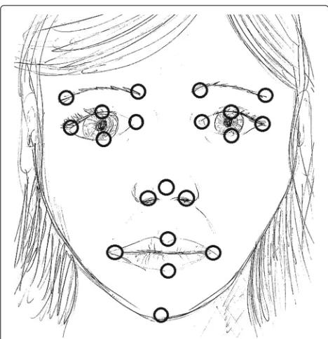
The video frame-based laughter detector starts with extracting the 20 face points, shown in Fig. 6, from each video frame using an algorithm from [49]. The uti-lized face points correspond to points used in [7]. Then, the dimensionality of each face point feature vector is
Fig. 6Face points. The 20 face points used as features for laughter-speech classification of MAHNOB Laughter dataset videos
reduced from 40 to 20 by principal component analy-sis (PCA). For frame-wise laughter likelihood estimates lv an NN is trained. It is built of 1 hidden layer of 10 neurons. All the neurons use tangential sigmoid transfer function, and mean squared error (MSE) loss function is applied for training. Video clipwise laughter likelihood is given as an average over the frame-wise values aslV =
1 NV
NV
τ=1lv(τ), whereNV is the number video frames in the clip.
4.1.2 CASA dataset
For video context change detection problem we use CASA database1 from [8]. Over 7 h of lifelog video material is filmed with a small pen camera, which operates at frame rate 15 frames/second and frame size 176×144 pixels. The stereo sound track is recorded by a pair of in-ear micro-phones with 44.1 kHz sampling rate and stored without compression. The database contains video material from 23 different types of environments.
For a context change detection task we created 30 video files of length 5–20 min. Each file is concatenated on aver-age of 105 clips of length 1–30 s from the video material of CASA database. The context—one of the 23 different environments included in the database—is kept the same for 1–5 successive clips, otherwise each clip is taken from a randomly selected video file. There are on average 42 context changes within each created video file. We run our tests using 6-fold cross-validation, where at each fold 5 files are reserved for testing and the remaining 25 files are used for system training.
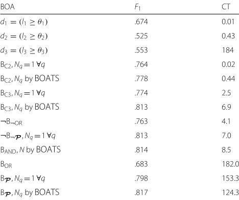
We use three different detectors to spot context changes in the created videos. Brief descriptions of the used detec-tors are given here, while the details of them can be found in [50]. The fastest one of the used detectors operates on the audio stream of the video. The audio is analyzed in frames of length 80 ms with 40 ms overlap of suc-cessive frames. From each audio frame, MFCC features are computed, and within a sliding window of 125 audio frames, mean and variance of 20 MFCC coefficients are computed. Transitions in these statistics are converted to a context change likelihoodl1for each audio frame. The computation time of scores l1 on a single CPU desktop computer is 0.8 ms per audio frame, that is 10 ms per one second of audio.
Two other utilized context change detectors operate on the image modality of the video. The faster one of the detectors on visual modality collects RGB histograms of video frames and produces the context change likelihood valuel2for each video frame according to the city block distance between adjacent RGB histograms. The compu-tation time ofl2 is about 29 ms per video frame, that is approximately 435 ms per one second of video.
The more accurate one of the used detectors on visual modality, proposed in [51], counts incidences of SIFT descriptor codebook elements within each video frame, and collects a SIFT histogram, i.e., so-called bag-of-words feature vector, for each video frame. The context change likelihood valuel3for each video frame is computed as the city block distance between SIFT-histograms of successive video frames. The computation time ofl3is about 12.3 s per video frame, that makes about 184 s per one second of video.
4.1.3 Performance measures
In the literature the performance of detectors is often presented by a receiver operation characteristic (ROC) curve. However, in our evaluations, we prefer the curve of precisionvsrecall(P-R curve) because in case of imbal-anced class distributions P-R curve is more faithful to the absolute number of erroneous classifications than the ROC -curve oftprin respect tofpr. To demonstrate the performance of a certain operating point of a detector, we use measures like accuracy,F1-score, and computational load.
4.2 Comparing BOA cascade to existing work in laughter vs speech classification
We compare the performance of the proposed BOA cas-cade to results we obtained with C5.0 -tree building algo-rithm [52] as well as results obtained by other authors in laughter vs speech classification, i.e., laughter detection, with the MAHNOB laughter dataset. For the task, we use a BOA detector
B(x;θ)=lA≥θA1
∨ N2
n=1
lA≥θA2,n
∧lV ≥θV2,n ,
(15)
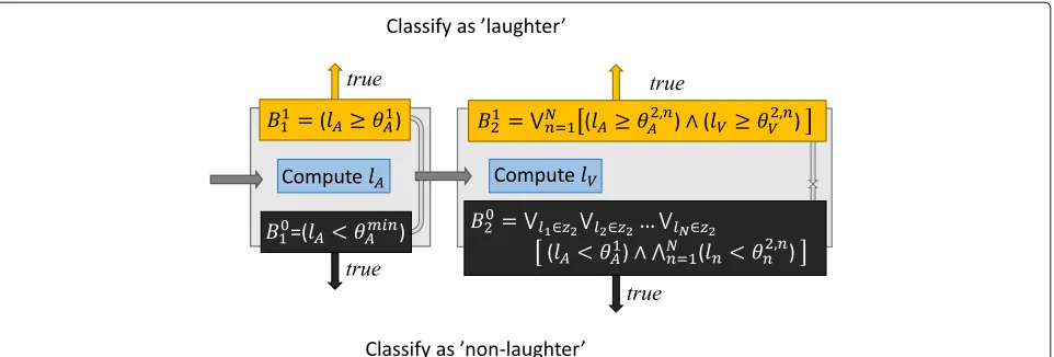
whose threshold parameters θA1, θA2,1, θV2,1, θA2,2, θV2,2, . . . ,θA2,N,θV2,N are learned by the proposed training algo-rithm. The Fig. 7 illustrates the BOA cascade of (15).
The computational load of acquiring lA from audio
stream is only a fraction of the load of computing lV from video frames. Thus, the ratio of samples that need the computation of lV reflects well the average computational load of classifying a sample with BOA cascade of (15).
Table 1 presents results with C5.0 tree building algo-rithm as well as those found in the literature in con-trast to our solution. We report performance numbers
with a BOA cascade of (15) with N = 1 and also
withNselected adaptively by the proposed training algo-rithm. The decision trees obtained with C5.0 algorithm [52] are converted to DNF-BF -form (15) and evaluated in cascaded manner similarly to BOA evaluation. The number N in the DNF-BF (15) of a tree varies accord-ing to the structure of the tree, which is given by the algorithm. The minimal leaf size of a tree was defined
by 10-fold cross validation using the training data. The boosted C5.0 forest contains 10 trees trained with differ-ent weightings by the training algorithm on training sam-ples. The classification of the forest is obtained via voting by the trees.
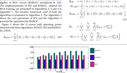
The C5.0 forest outperforms all the other solutions in terms of classification accuracy, whereas the performance of single C5.0 tree is comparable to performance obtained with BOA classifiers. When a C5.0 tree is evaluated in cas-caded manner, very similar computational savings as with a BOA cascade are obtained. Both the BOA detectors out-perform the solutions of [53, 54], albeit the classifier in [54] is trained with another database, which likely explains its lower detection accuracy. The results obtained by [55] reach similar accuracy andF1-scores than our BOA cas-cades, but their result is not fully comparable as they use only a subset of 15 speakers out of 22 used by all the other authors. However, the computational load of our solution is significantly lower, compared to all these other mul-timodal solutions. With our BOA cascade of (15) with N=1, only 11% of samples needed the computation oflV, thus it is about nine times faster than the other solutions. The BOA cascade of (15) withNselected by the proposed training algorithm reaches slightly higher accuracy than the reference solutions while being still three times faster than them.
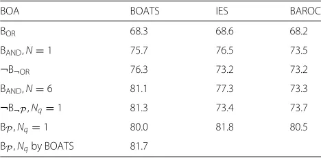
4.3 Comparing training algorithms for BOA combination We use the CASA lifelog data and the context change detection task for illustrating the capability of the pro-posed training algorithm to find successful operating points for a BOA combination. For context change detec-tion we use BOA combinadetec-tions built of three detectors,
Fig. 7Symmetrical BOA cascade for laughter detection. Symmetrical BOA cascade, which is capable of making early classification to both classes, realizing of BOA (15) for laughter detection. The conjunction setz2= {lA,lV}and the thresholdθAminisθAmin=min
θ1
A,θA2,1,θA2,2,. . .,θA2,N
.B0 2
containsK=2Nconjunctions, where the first threshold comparison is alwaysl A≥θA1
. The comparisons indexed byn=1. . .Noperate either on
lAorlVaccording to binary (M2-ary)N-digit representation of the conjunction indexk=1. . .K, bin(k). If then:th digit of bin(k)is 0,lAis used, andlV