Small-angle X-ray scattering study on nanostructural changes with water content in red pine, American pine, and white ash

ORIGINAL ARTICLE

Weidong Cheng · Xueqing Xing · Dehong Wang Kunhao Zhang · Quan Cai · Guang Mo

Zhongjun Chen · Zhonghua Wu

Small-angle X-ray scattering study on nanostructural changes with water

content in red pine, American pine, and white ash

Abstract Wood is a highly sophisticated and multihierarchi-cal material. The nanosmultihierarchi-cale structures in natural cell walls of red pine, American pine, and white ash specimens were investigated using the small-angle X-ray scattering (SAXS) technique. A tangent-by-tangent method was used to analyze the SAXS data. The results demonstrate that the multihierarchical scatterers in the three specimens can be divided into two dominant components, i.e., a sharp compo-nent and a wide compocompo-nent. The sharp compocompo-nent mainly corresponds to the contribution of cellulose microfi brils, and its size is almost unaffected by the water content. However, the wide component includes voids or micro-cracks and cellulose microfi bril aggregates; its size changes, refl ecting swelling and water accumulation in the voids or microcracks. Because of the different morphological fea-tures of the cell walls, softwood (red pine and American pine) displays different tendencies from hardwood (white ash) in terms of changes in the wide component with water content: the average scatterer size of the wide component has an incremental tendency with the water content in soft-wood, but it has a descending tendency in hardwood. Fractal analysis further revealed that in white ash the surface of scatterers is coarser and the scatterers form more compact nanostructures than in the two pine woods. All this nano-structural information can be used to explain well the dif-ference of swelling behaviors between the two pines and the white ash.

Key words Small-angle X-ray scattering · Nanostructure · Water content · Wood

Introduction

It is well known that natural wood is a highly sophisticated and multihierarchical material. There are four distinct length scales of hierarchical ordering, i.e., the macroscopic level of tissue structure, the microscopic level of cell struc-ture, the submicroscopic level of cell-wall organization, and the nanoscopic level of cell-wall polymer assembly. The cell wall is a laminated structure in which the thickest S2 layer occupies 70%–80% of the volume of the cell wall. Due to the hygroscopic property of wood materials, their changes in microstructure with water content are of great interest. It is known that absorbed moisture will cause macroscopi-cally perceptible changes of wood materials, such as swell-ing1

or decay.2

However, the water-absorbing process is mostly associated with the ultrastructure and nanostructure in the texture of wood. Clarifying the nanostructures in wood and their changes with water content is very impor-tant in industrial and environmental applications of wood materials.

There have been a number of studies3–12

about the micro-structural changes in wood with water content, but the con-clusions on water storage and transport in woods are inconsistent. Christensen13

pointed out that the uptake of water by plants involves two stages: wetting at capillary surfaces followed by molecular penetration and swelling of the solid phase. Simonaho14

observed the infl uence of tap water on the cell wall and cavities of Scots pine, and found that the added water was located inside the cell wall matrix and caused macroscopic swelling of the timber sample. Several research groups15–17

thought that wood eventually reaches an equilibrium state when the moisture content in wood increased continually, and the cell walls cease further swelling as liquid water begins to accumulate in the lumens and voids. Stamm18

claimed that the absorbed water was inaccessible to the interior of the cellulose crystallites of the cell wall and was only confi ned in the amorphous regions or the surface of cellulose crystallites. The imbibition16,19 of water in wood was found to push apart the polysaccharide molecules. Ma and Rudolph20

concluded that the main Received: October 25, 2010 / Accepted: May 18, 2011 / Published online: August 7, 2011

DOI 10.1007/s10086-011-1202-1

W. Cheng · X. Xing · D. Wang · K. Zhang · Q. Cai · G. Mo · Z. Chen · Z. Wu (*)

Beijing Synchrotron Radiation Facility, Institute of High Energy Physics, Chinese Academy of Sciences, PO Box 918, Bin 2-7, Beijing 100049, P. R. China

Tel. +86-10-88235982; Fax +86-10-88235982 e-mail: [email protected]

W. Cheng · X. Xing · D. Wang · K. Zhang

contributors to water adsorption were the hydroxyl groups of the carbohydrates from cellulose and hemicelluloses in cell walls. Berry and Roderick15

and Deshpande et al.21 reported that much of the water in wood was held in the S2 layer and tracheids. Kang and Chung22

investigated water transport in wood specimens and found that most species had unimodal pore distributions; however, aspen had a bimodal pore distribution. Recent research23

obtained the nanocrystallite deformation of cellulose microfi brils in spruce wood on dehydration and rehydration. Although all these previous studies are very helpful in understanding the water-absorbing process and the nanostructural changes with water content in wood, due to the structural complex-ity of wood and possible species differences, the swelling mechanism of wood is still ambiguous, and information about the nanostructural changes in wood with water content is still scarce. More studies are necessary for an unambiguous “image” of absorption and water-transport processes in wood.

Usually, absorbed water in wood is in three possible states: as vapor in the gas-fi lled voids, as free or bulk water in the voids, and as bound water in the cell wall matrix. The absorption of water in wood causes nanoscale electron-density changes. The small-angle X-ray scattering (SAXS) technique24,25

is quite suitable for the nondestructive study of nanoscale structures. For example, SAXS has been suc-cessfully employed to investigate the nanostructure26–29

in the natural wood cell of Picea abies. The nanopore contribu-tion was successfully separated from the cell wall matrix with SAXS data analysis. Cellulose microfi brils (CMFs) of

Picea abies were confi rmed to exist with a uniform fi bril

diameter only, but the diameters of CMFs obtained by dif-ferent research groups range approximately from 2 to 4 nm, and the structure function describing the relative arrange-ment of the cellulose fi bers was obtained for the native cell wall. The scanning SAXS30

technique was also successfully used to identify the fi ber direction and size. In this article, SAXS is used to detect the scatterer sizes and their nano-structural evolution with water content in native red pine (Pinus koraiensis), American pine (Pinus elliottii), and white ash (Fraxinus americana). We hope that this study helps elucidate the swelling mechanism and the nanostruc-tural differences between softwood (red pine, American pine) and hardwood (white ash).

Experiments and methods

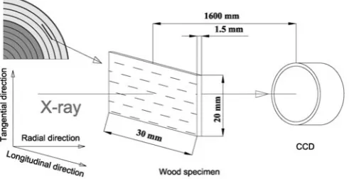
Three types of wood specimens (native red pine, American pine, and white ash) were carefully prepared for SAXS measurements. For all three species, samples were cut out from the sapwood at breast height without resin canals or knots. The dimensions of the samples were approximately 20 mm in the tangential direction, 30 mm in the longitudinal direction, and 1.5 mm in the radial direction. Each sample had an apparent volume of V0 = 0.9 ± 0.04 cm

3

. These slices were taken from a single annual ring consisting of early-wood and lateearly-wood, but the samplings were consciously

approximated to the earlywood region of the annual ring. A schematic of the sampling and the wood specimen is shown in Fig. 1. For each wood type, one slice was cut out in the same way. The three wood samples were polished with 1000-mesh sandpaper without chemical treatment and then were washed with deionized water. Finally, these speci-mens were kept in a desiccator at 150°C and dried until the weight was constant. In our wood slices, the CMFs in the S2 wall were approximately parallel to the longitudinal direc-tion of the stems.

Deionized water was directly added to the specimen sur-faces by using a Gilson pipette with scale of 0–100 μl. Water addition was controlled and accumulated to 0.04, 0.12, 0.20, 028, 0.36, 0.44, 0.60, and 0.68 ml. At the same time, the water was uniformly dropped on the samples and then spread onto the whole surface. In order to add more water into the specimens, the red pine and white ash specimens were also immersed into the deionized water for 7, 20, 30, 45, and 65 min. Then these specimens were enwrapped with imper-meable polyethylene fi lm and closed in vessels for water homogenization in the specimens and to prevent the water from volatilization. About 15 min later, the possible excess water on the specimen surface was removed with fi lter paper. Before SAXS measurements, the water contents absorbed by the specimens were evaluated by comparing the specimen weight after and before adding water with a Mettler Toledo XS205 electronic balance with an accuracy of 10 μg. The relative volume percentage of moisture in the specimen was given by the formula: x = V/V0 = m/V0, where V = m/ρ, is the volume of absorbed water, m is the weight of the absorbed water, and ρ = 1 g/cm3

, the mass density of water.

Because the water was directly added to the surface of the specimens, the moisture distribution in the radial direc-tion (i.e., the thickness direcdirec-tion) of specimens cannot be homogeneous initially. From the surface to the specimen center, a gradient distribution of water content is present. This unevenness of moisture in the sample thickness is the main source of experimental error. If the homogenization time is suffi cient, a homogeneous moisture distribution in the thickness direction of the specimens will hopefully be achieved. In our experiments, the exact distribution of water in the specimens was unknown. Moisture distributions12,16

Fig. 1. Schematic of wood samplings and small-angle X-ray scattering

(a) (b)

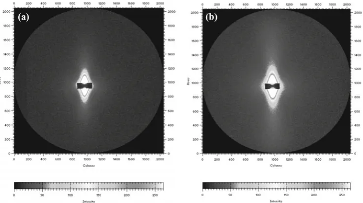
Fig. 2. Two-dimensional SAXS

patterns of American pine in the dry state (a) and in the hygroscopic state with a volume percentage of moisture of 18.4% (b)

have been researched for Scots pines and Norway spruce. It was found that moisture distribution was uneven along the direction of sample thickness after short-term free water soaking, but a fl at gradient of moisture distribution was obtained when the sample was immersed in water for 4 h. That is to say, the moisture distribution was approximately uniform in the plane perpendicular to the thickness direc-tion. Therefore, the unevenness of moisture in these planes perpendicular to the incident X-ray direction can be omitted in our samples, because the incident X-ray spot is much smaller than the specimen surface area. Before each SAXS measurement, specimen homogenization was carried out for at least 15 min. From adding water to the specimen to fi nishing all SAXS measurements with different water con-tents took a few hours. Therefore, the specimens were in a nonequilibrium state.

The SAXS patterns of the specimens with different water contents were collected using beam line 1W2A of the Beijing Synchrotron Radiation Facility (BSRF) with an incident X-ray wavelength of 0.154 nm. The storage ring was operated at 2.5 GeV with a current of about 200 mA. A Mar 165 two-dimensional charge-coupled device (CCD) detector with 2048 × 2048 pixels was positioned perpendicu-larly to the incident beam with a detector–sample distance of 1600 mm, and this was calibrated with a standard sample. During the SAXS measurements, the longitudinal direction of wood growth was placed in the horizontal plane, and the incident X-ray beam was along the radial direction, as shown in Fig. 1. Because SAXS is a statistical average method over the irradiated volume of specimens, one SAXS pattern for each scattering experiment at a specifi ed mois-ture content was enough to get the statistical average infor-mation for nanoscale scatterers. These measured SAXS patterns were fi rstly transformed into one-dimensional SAXS curves with the software Fit2D.31

After removal of the instrumental background, the SAXS intensities were normalized to the primary beam intensity.

Results and discussion

As examples, the SAXS patterns of American pine in the dried state and in the hygroscopic state with a volume per-centage of moisture of 18.4% are, respectively, shown in Fig. 2a and Fig. 2b. Clearly, the water-absorbed sample has a wider SAXS intensity distribution. Without further SAXS data analysis, it can be concluded that the scatterer sizes in the wood specimens change with the absorbed water content. Figure 2 shows clearly that both SAXS patterns have a double-wedge shape. Similar SAXS patterns were also found for the other wood specimens. As expected, these SAXS patterns imply that the wood material is anisotropic, and the longitudinal direction has a larger particle size than the tangential direction.

According to the specimen orientation, the SAXS signal recorded in the vertical direction of the detector refl ects structural information of the tangential direction of the wood specimens. In order to ascertain the scatterer size and distribution, the SAXS data were analyzed using the model-independent tangent-by-tangent (TBT)32–34

method, which has been successfully applied to decompose the contribu-tions of nanoparticles with different sizes. For a polydis-perse particle system, the SAXS intensity with Guinier approximation can be described as:

I q Ie N Rg V R eg dR

q R g

g

( )=

∫

2 2

(1)

where q = 4λsinθ/λ, θ is half the scattering angle, λ is the incident X-ray wavelength, Rg, N, V, and ρ are the radius of gyration, the number of particles with Rg, the volume of a particle with Rg, and the electron density, respectively. Ie is the scattering intensity of one electron. For a system with only a few discrete particle sizes, the integral in Eq. 1 can be discretized as the following summation:

I q I N n ee I N n e I N n e

q R e

q R

e i i q Ri

( )= 1 1 − + − + + −

2 3

2 2

2 3 2 3

2

0.1 1 100

102 104 106 108

1010

1012 1014

(a)

28.4%±1.3% 27.1%±1.2% 26.1%±1.2% 25.7%±1.1% 24.2%±1.1% 19.3%±0.9% 16.0%±0.7% 12.0%±0.5% 9.7%±0.4% 2.9%±0.1% Dryness

SAXS Intensity (a. u.)

q

(nm

)

0.1 1

10-1 101 103 105 107 109

1011 _(b)

19.9%±0.9% 18.4%±0.8%

17.1%±0.8% 15.0%±0.7% 12.7%±0.6% 9.1%±0.4% 3.3%±0.1% Dryness

SAXS Intensity (a. u.)

q

(nm

)

0.1 1

100 102 104 106 108 1010 1012 1014 1016

(c)

53.4%±2.4% 55.7%±2.5% 53.9%±2.4%

51.0%±2.3% 46.9%±2.1% 43.6%±1.9% 39.4%±1.8% 34.4%±1.5% 26.2%±1.2% 17.2%±0.8% 10.2%±0.5% 3.7%±0.2% Dryness

SAXS Intensity (a. u.)

q

(nm

)

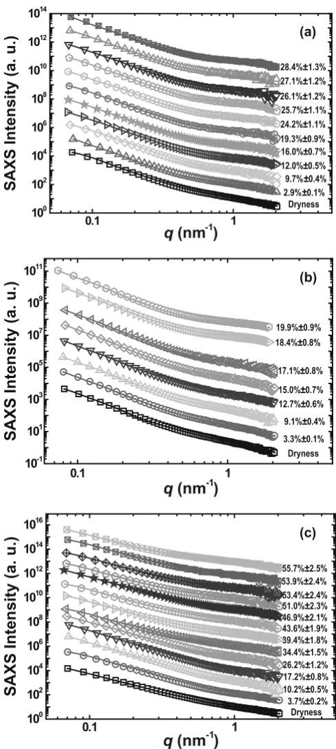
Fig. 3a–c. Comparison between the experimental SAXS intensities

(symbols) and the calculated values (solid lines). a The red pine speci-men. From bottom to top, the volume percentages (V/V0) of absorbed

water are 0%, 2.9%, 9.7%, 12.0%, 16.0%, 19.3%, 24.2%, 25.7%, 26.1%, 27.1%, and 28.4%. b The American pine specimen. From bottom to top, the volume percentages (V/V0) of absorbed water are 0%, 3.3%, 9.1%,

12.7%, 15.0%, 17.1%, 18.4%, and 19.9%. c The white ash specimen. From bottom to top, the volume percentages (V/V0) of absorbed water

are 0%, 3.7%, 10.2%, 17.2%, 26.2%, 34.4%, 39.4%, 43.6%, 49.6%, 51.0%, 53.4%, 53.9%, and 55.7%. The SAXS curves are offset in verti-cal direction for clarity

where i represents the ith size level. ni is the electron number in the particle with gyration radius Ri. When q = 0, the SAXS intensity is given as:

I( )0 =K1+K2+ + Ki (3)

where Ki = IeNin 2 i = IeNiρ

2 Vi

2 _{= I} eρ

2

NiViVi = Ieρ 2

WicRi 3

is the intercept of the ith tangent on the ordinate. The gyration radius Ri can be obtained from the slope of the ith tangent. Therefore, the volume percentage is given by:

W W W K

R K R

K R

i

i

i

1 2

1 1 3

2 2

3 3

: :: = : :: (4)

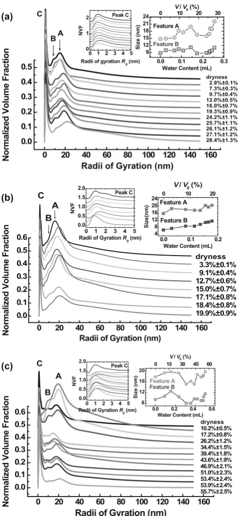
The experimental SAXS intensities and the values cal-culated using the TBT method are shown in Figs. 3a, 3b, and 3c, respectively, for the red pine, American pine, and white ash specimens. The SAXS fi tting curves are all in excellent agreement with the experimental data. The normalized volume fractions (NVFs) were obtained for the three wood specimens, as shown in Fig. 4. Each of the NVFs of the three wood specimens can be divided into two distinct parts: a sharp component (feature C) with a smaller particle size and a wide component (dominant features A and B) with a larger particle size.

In the three wood specimens, feature C is less changeable with variation of the volume percentage of moisture. The most probable values of the gyration radius Rg are, respec-tively, 1.1, 1.1, and 1.2 nm, with slight fl uctuations, for the sharp components in red pine, American pine, and white ash specimens. The average values of the sharp components are, respectively, around 2.3 ± 0.4, 2.2 ± 0.3, and 2.2 ± 0.6 nm for the red pine, American pine, and white ash specimens. Evidently, even for the sharp components, the respective scatterer size is also not a single value for the three specimens.

It is well known that the nanoscopic cell-wall polymer assembly consists of CMFs, amorphous hemicellulose, and lignin. The CMFs of wood specimens are anisotropic and can be approximately described as cylindrical scatterers. Their axial direction is along the longitudinal direction, and their radial direction is perpendicular to the longitudinal direction. According to the orientation of specimens rela-tive to the incident X-ray beam, a wafer model can be used to evaluate the diameter of the cylindrical scatterers. The physical diameters are obtained as 3.1, 3.1, and 3.4 nm for the most probable contribution of the sharp components in red pine, American pine, and white ash specimens, respec-tively. These values are in excellent agreement with the sizes21,27

of CMFs in previous reports. Therefore, we can attribute feature C to the contribution of CMFs and can conclude that the size of CMFs is approximately unchange-able with the volume percentage of moisture. This result demonstrates that the water-absorbing process or the increase of the volume percentage of moisture does not alter the size of CMFs in the three wood specimens studied. In other words, there is almost no interaction between water molecules and cellulose molecules inside CMFs. This con-clusion confi rms the fi ndings of a previous report18

0.0 0.1 0.2 0.3 9 12 15 18 21

24 0 10 20 30

0 20 40 60 80 100 120 140 160

0.0 0.1 0.2 0.3 0.4 0.5 (a)

Normalized Volume Fraction

Radii of Gyration (nm)

dryness 2.9%±0.1% 7.3%±0.3% 9.7%±0.4% 12.0%±0.5% 16.0%±0.7% 19.3%±0.9% 24.2%±1.1% 25.7%±1.1% 26.1%±1.2% 27.1%±1.2% 28.4%±1.3% Feature B C Feature A BA Size (nm)

Water Content (mL) 0 1 2 3 4 5

0 1

2 Peak C

NVF

Radii of gyration Rg (nm)

V / V0 (%)

0.0 0.1 0.2 4

8 12 16 20

24 0 10 20

0 20 40 60 80 100 120 140 160

0.0 0.1 0.2 0.3 0.4 0.5 0.6 dryness 3.3%±0.1% 9.1%±0.4% 12.7%±0.6% 15.0%±0.7% 17.1%±0.8% 18.4%±0.8% 19.9%±0.9%

Normalized Volume Fraction

Radii of Gyration (nm)

Feature B Feature A C B A Size(nm)

Water Content (mL) 0 1 2 3 4 5

0.0 0.5 1.0 1.5 2.0 Peak C NVF

Radii of Gyration Rg (nm)

(b)

V / V 0 (%)

0.0 0.2 0.4 0.6

8 12 16 20

0 15 30 45 60

0 20 40 60 80 100 120 140 160

0.0 0.1 0.2 0.3 0.4 0.5 0.6

Normalized Volume Fraction

Radii of Gyration (nm)

C Feature B B Feature A A Size (nm)

Water Content (mL)

0 1 2 3 4 5

0.0 0.5 1.0 1.5

2.0 V / V0 (%)

Peak C

NVF

Radii of Gyration Rg (nm)

dryness 10.2%±0.5% 17.2%±0.8% 26.2%±1.2% 34.4%±1.5% 39.4%±1.8% 43.6%±1.9% 46.9%±2.1% 51.0%±2.3% 53.4%±2.4% 53.9%±2.4% 55.7%±2.5% (c)

Fig. 4a–c. Normalized volume fraction of scatterers. a The red pine

specimen. From top to bottom, the volume percentages (V/V0) of

absorbed water are 0%, 2.9%, 7.3%, 9.7%, 12.0%, 16.0%, 19.3%, 24.2%, 25.7%, 26.1%, 27.1%, and 28.4%. b The American pine speci-men. From top to bottom, the volume percentages (V/V0) of absorbed

water are 0%, 3.3%, 9.1%, 12.7%, 15.0%, 17.1%, 18.4%, and 19.9%. c The white ash specimen. From top to bottom, the volume percentages (V/V0) of absorbed water are 0%, 10.2%, 17.2%, 26.2%, 34.4%, 39.4%,

43.6%, 46.9%, 51.0%, 53.4%, 53.9%, and 55.7%. The insets enlarge feature C or show the size evolutions of feature A and feature B with the water content (bottom abscissa) or the volume percentage (top

abscissa)

units21,35–37

with a diameter of about 7–30 nm. Terashima et al.38

also suggested that the cross section of the composite unit [CMF bundle + hemicellulose–lignin module] was square with a side of 18 ± 1 nm, with a possible parallelo-gramic or hexagonal cross section of a bundle of CMFs of 12 ± 3 nm across. In addition, there were also some molecule-scale cavities and voids15,25,27

in the hemicellulose– lignin matrix, which could divide the cell wall into smaller regions. It is these smaller regions and the smaller CMF aggregations that can contribute partially to the sharp com-ponents of the three wood specimens, which results in an asymmetrical distribution in the NVFs of the sharp components.

The wider components in the NVFs of the three wood specimens are variable. The much wider distribution of scat-terer sizes can be attributed to the contribution of polydis-perse scatterer sizes (for example, the possible voids or microcracks as well as the CMF aggregates) and the gradi-ent distribution of moisture. Features A and B belong to the wide component. They are, respectively, located at 17.8 nm and 9.4 nm for the initial state (dryness) of the white ash specimen, 15.8 nm and 6.4 nm in the initial state of the American pine specimen, and 14.8 nm and 8.8 nm in the initial state of the red pine specimen. The large difference of gyration radii between features A and B cannot be attrib-uted to the swelling difference in the specimen thickness because the gradient of moisture is approximately continu-ous39

in the thickness direction of specimens. Thus, two dis-tinct gyration radii within the wide component illustrate that a multimodal size distribution exists in the three wood specimens. This result is not in agreement with previous research22

by Kang and Chung who claimed that most species had unimodal pore distributions, except for aspen, which had a bimodal pore distribution. The changes of gyra-tion radii Rg of features A and B with water content (bottom abscissa) or volume percentage of moisture (top abscissa) are shown in the insets of Fig. 4. In general, the sizes of features A and B increase with increasing water content, presenting a swelling behavior versus volume percentage of moisture. Based on the most probable sizes of features A and B, a reasonable conjecture is that features A and B contain, respectively, the contribution of the CMF bundles and the surrounding tubular hemicellulose–lignin matrix (HLM). Under the infi nite cylinder hypothesis, the physical diameters of CMF bundles are, respectively, about 25, 22, and 21 nm for white ash, American pine, and red pine, and the corresponding thicknesses of HLM are, respectively, about 13, 9, and 12 nm. These values are approximately twice those of Terashima’s model.38

The initial average sizes of the detectable scatterers in the wide components are estimated to be 40 ± 3, 41 ± 2, and 38 ± 2 nm for the dry states of red pine, American pine, and white ash specimens, respectively. Evidently, the wide com-ponents not only contain the contribution of CMF bundles and HLM, but also contain other scatterers, such as voids or microcracks, or even the lumens. Nanocrystallite defor-mation of CMFs in the S2 layer of spruce wood tracheids was observed23

of the extra water that created enormous stresses in the cell wall and caused longitudinal contraction, lateral expansion, and changes in the monoclinic angle of the cellulose unit cell during drying of wood fi bres. Because the whole cell wall material is destabilized when drying wood beyond the fi ber saturation point, some voids or microcracks with larger sizes can be formed and contribute to the wide component.

We also noted the following variational tendency of fea-tures A and B. At fi rst, the sizes of feafea-tures A and B increase with the volume percentage of moisture; however, as the water content in the specimens reaches certain values, the sizes of features A and B begin to decrease. With further increase of water content, the sizes of features A and B increase again. From Figs. 4a and 4c, it can be found that there is size “shrinkage” in features A and B when the volume percentage of moisture is around 23% for the red pine specimen, or is around 35% for the white ash specimen. An explanation for this phenomenon is that when water penetrates into a wood specimen, a small quantity of water is stored in the cell wall matrix. With the increase of water in the specimens, liquid water begins to accumulate in the lumens and voids or microcracks. At this stage, the nanoscale voids or microcracks gradually fi ll with water. Therefore, the average size of scatterers (liquid water and the unfi lled por-tions of the voids) with respective uniform electron density would fi rst decrease and then increase, presenting a concave-down feature in the curve of scatterer size versus volume percentage of moisture, as shown in the insets of Figs. 4a and 4c. In this case, the size “shrinkage” of features A and B does not mean that the wood specimens were contracting in the water-absorbing process. It is simply the cumulative progress of water in the nanoscale voids or microcracks and lumens. The volume percentage of moisture related to the “shrinkage” is larger in white ash (~35%) than in red pine (~23%). Red pine and white ash can be classifi ed as soft-wood and hardsoft-wood, respectively. Usually, softsoft-woods have thinner cell walls and larger lumens, while hardwoods have thicker cell walls and narrower lumens. Before the water accumulates in the lumens and voids, the thicker cell wall can hold more water in the initial water-absorbing process so that the “shrinkage” occurs at a larger volume percentage of moisture in white ash than in red pine.

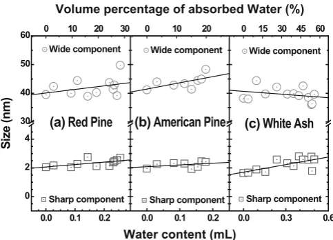
Figure 5 illustrates the evolutionary processes of the average Rg versus the absorbed water content (bottom abscissa) or the volume percentage of moisture (top abscissa). In the cases of the red pine and the American pine specimens, the Rg of the sharp component is almost unchanged with the absorbed water content, but the Rg of the wide component increases slightly with the volume per-centage of moisture. However, in contrast to the red pine and American pine specimens, the white ash specimen has a faster increase in average Rg of the sharp component with water content. Also, the average Rg of the wide component shows a decreasing tendency with the volume percentage of moisture. These different characteristics of the average

Rg versus water content can be ascribed to the different nanostructures in red pine, American pine, and white ash. Both pine specimens are softwoods; they have cells with an

open lumen and thinner cell walls. In contrast, the white ash specimen is a hardwood; its cells are thick-walled with a narrower central lumen. In addition, the nanostructure in the white ash is more compact, which creates better strength and bending tenacity compared with the pine wood. For the softwoods (red pine and American pine), the absorbed water exists mainly in the nanoscale voids or microcracks of cell walls and the larger lumen. Because the cell wall is thinner and with looser structures, the swelling, including the expansion of nanoscale voids or microcracks, makes less contribution to the sharp component, which results in the relatively constant Rg of the sharp component. At the same time, the expansion of the lumen and voids or micro-cracks can cause the increasing Rg of the wider component. But in hardwood (white ash), more water enters the amor-phous hemicellulose and lignin surrounding CMFs. Because of the thicker cell wall and the more compact structures, the swelling of cell walls and the expansion of nanoscale voids or microcracks make a larger contribution to the sharp component. Some small amount of water formed at the cell wall will contribute partially to the sharp compo-nent, causing an increase of average Rg of the sharp com-ponent. Simultaneously, the swelling of the thicker cell walls probably invades the volume of the central lumen (including the voids or microcracks) so that the size of the wider component decreases with the volume percentage of moisture. We believe that the size of water droplets formed in the lumens increases with the increase of water content. Thus, it is the difference of nanostructures between pines and white ash that leads to different trends in average Rg, as shown in Fig. 5.

From the above analysis, we confi rmed that the water content has a prominent infl uence on the size changes of features A and B, which correspond to the contribution of CMF aggregates, voids or microcracks, and water droplets

Fig. 5. Average radii of gyration changes with the water content

(bottom abscissa) or the volume percentage of absorbed water in the specimens (top abscissa) for the sharp component (squares) and the wide component (circles) in the red pine specimen (a), the American pine specimen (b), and the white ash specimen (c). Lines are the linear best fi t values

0.0 0.1 0.2

0 2 4 30 40 50 60

0.0 0.1 0.2 0.0 0.3 0.6

0 10 20 30 0 10 20 0 15 30 45 60

Wide component Wide component Wide component

Sharp component Sharp component

Sharp component

(a) Red Pine

Size (nm)

Volume percentage of absorbed Water (%)

Water content (mL)

0.0 0.2 0.4 20 40 60 0

1 30 40 50

0.0 0.3 0.6 0.0 0.3 0.6 20 40 60

(a)

Water content (mL // min)

(b)

(c)

D_m

D_m

D_S

D_S

D_m

D_S

D_m

D_m

D_m

D_S

D_S

D_S

0 10 20 30 0 10 20 0 15 30 45 60

Volume percentage of absorbed water in the pecimens (%)

White Ash American Pine

Red Pine

American Pine

Red Pine White Ash

Absorbed Water content in the specimens (mL)

Fractal Dimension

(c1)

(c2)

(b2)

(a2)

(b1)

(a1)

ln

I

(

q

)

0.0 0.1 0.2

0.0 0.1 0.2 0.3

0.8 1.2 1.6 2.0 2.4 2.8 3.2

0.0 0.2 0.4 0.6

-3 -2 -1 0 1

-2 0 2 4 6 8 10

-3 -2 -1 0 1 -3 -2 -1 0 1

lnq

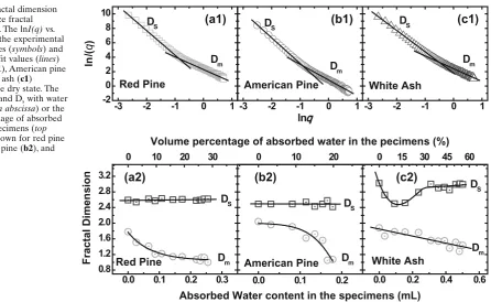
Fig. 6. Mass fractal dimension

(Dm) and surface fractal dimension (Ds). The lnI(q) vs. lnq plots show the experimental SAXS intensities (symbols) and the linear best fi t values (lines) for red pine (a1), American pine (b1), and white ash (c1) specimens in the dry state. The changes of Dm and Ds with water

content (bottom abscissa) or the volume percentage of absorbed water in the specimens (top

abscissa) are shown for red pine

(a2), American pine (b2), and white ash (c2)

in the interior of lumens. For these detectable scatterers in the wider component, the average sizes over specimens with different water contents were estimated to be 42 ± 4, 44 ± 3, and 40 ± 3 nm; the standard deviations of the regression lines were 3, 2, and 2 nm for red pine, American pine, and white ash, respectively. Although softwood (red pine and American pine) has a larger swelling rate than hardwood (white ash), the average sizes of scatterers in the wide com-ponent over the water-absorption process hardly change, if considering the standard deviation; however, the change tendencies of the regression lines are still credible.

It is well known that more voids and cavities are pro-duced40

with the increase of water uptake. On the basis of Fig. 5, we can conclude that the swelling of softwood (red pine and American pine) is mainly dependent on the expan-sion of voids or microcracks and water droplet size in lumens with the volume percentage of moisture, which leads to more marked swelling behavior. However, hardwood, for example white ash, has a more compact structure and thicker cell walls. Its swelling depends mainly on the expan-sion of cell walls with the volume percentage of moisture. The compression of the larger lumens compensates partially the swelling of the amorphous hemicellulose and lignin in the cell wall. As a result, white ash presents a lower swelling value. These behaviors are consistent with the swelling phe-nomena of softwood and hardwood.

In addition to the radius of gyration, fractal dimension41,42 is also a crucial parameter to describe nanoscale structures. SAXS data can be employed to analyze the fractal structure. The fractal dimension D is just used to quantify the changes of the mass or the surface of scatterers. In such a case, the SAXS intensity can be described as:

I q( )=Cq−α (5)

This change implies that the voids or microcracks in white ash specimen have an increasing tendency at the initial stage. Subsequently, the swelling of the cell wall invades partially the volume of the lumen, which causes a compres-sion of the larger voids or microcracks and results in a slow increase of the surface coarseness. The larger Ds values of the white ash specimen indicate that the coarseness of the scatterer surface in the cell walls of white ash is greater than that in the other two specimens. Such a coarse surface might compensate partially the swelling of the wood specimen with the volume percentage of moisture.

The morphological differences of cell wall polymers between softwood and hardwood are mainly focused on the thickness of the cell wall and the lumen size, which refl ect the density of wood. Although the three wood speci-mens all have CMF bundles surrounded by amorphous hemicellulose–lignin matrix (HLM) in the S2 layer of cell walls, the sizes of CMF bundles and the HLM thickness are different. Some molecule-scale cavities exist in the HLM, and nanoscale microcracks exist in the S2 layers of cell walls due to the drying process. Absorbed water can enter these microcracks and the lumens to form water droplets. Some microcracks and the water droplets could be larger than 40 nm. The size of water droplets has an obvious effect on the wide component changes with water content. The morphological features of the cell wall deter-mine the swelling behavior of the wood. However, the nanoscopic morphological features of cell walls could be changed in the drying process of wood due to the weather-ing of hemicellulose or reannealweather-ing of cellulose or the high surface tension of water on CMFs. The rehydration process of dry wood and the dehydration process of green wood are not reversible. That is to say, the water content distribu-tion could be different between the swelling process of dried wood and the drying process of green wood. The difference of nanoscopic characteristics with water content between dehydration and rehydration processes of wood is still ambiguous. Comparing the swelling process of dried wood with the drying process of green wood is worthy of further study in future. It promises to give additional insight into the differences in nanoscopic characteristics between dried samples and never-dried samples.

Conclusions

The nanostructural changes with absorbed water content in red pine, American pine, and white ash specimens were studied using the SAXS technique. The obtained results were compared among the three wood specimens and can be summarized as follows. The nanostructures in the three wood specimens consist of a sharp component and a wide component. The main contribution to the sharp component comes from CMFs, the size of which remain constant (~3 nm) during the whole water-absorbing process. There is no obvious interaction between water molecules and cel-lulose molecules inside CMFs. The wide component includes voids, microcracks, and CMF aggregates. The size change of

the wide scatterer component is related to the swelling behavior. A different nanostructural evolution was found between softwood (red pine and American pine) and hard-wood (white ash). In softhard-wood, the size of the wide scatterer component has an incremental tendency with the volume percentage of moisture, but it has a descending tendency in hardwood. The absorbed water exists mainly in the open lumens in softwood, or in the amorphous hemicellulose and lignin surrounding CMFs in hardwood. The surface or inter-face of the scatterers is coarser in hardwood (white ash) than in softwood (red pine and American pine). Such a coarse surface of scatterers compensates partially the swell-ing caused by the absorbed water. The structural looseness of the scatterers increases with the increase of the volume percentage of moisture in all three wood species.

Acknowledgments This work was supported by the National Natural

Science Foundation of China with Grant Nos. 10374087 and 10835008, the Knowledge Innovation Program of the Chinese Academy of Sciences (Grant No. KJCX3-SYW-N8), and the Momentous Equip-ment Program of the Chinese Academy of Sciences (Grant No. YZ200829).

References

1. Murata K, Masuda M (2006) Microscopic observation of transverse swelling of latewood tracheid: effect of macroscopic/mesoscopic structure. J Wood Sci 52:283–289

2. Chirkova J, Irbe I, Andersons B, Andersone I (2006) Study of the structure of biodegraded wood using the water vapour sorption method. Int Biodeter Biodegr 58:162–167

3. Ashori A, Sheshmani S (2010) Hybrid composites made from recy-cled materials: Moisture absorption and thickness swelling behav-ior. Bioresource Technol 101:4717–4720

4. Berthold J, Rinaudo M, Salmen L (1996) Association of water to polar groups: estimations by an adsorption model for ligno-cellulose materials. Colloid Surf A: Physicochem Eng Aspects 112:117–129

5. Hartley ID, Kamke FA, Peemoeller H (1992) Cluster theory for water sorption in wood. Wood Sci Technol 26:83–99

6. Oliveira FGR, Candian M, Lucchette FF, Salgon JL, Sales A (2005) A technical note on the relationship between ultrasonic velocity and moisture content of Brazilian hardwood (Goupia glabra). Build Environ 40:297–300

7. Qing H, Mishnaevsky L (2009) Moisture-related mechanical prop-erties of softwood: 3D micromechanical modeling. Comput Mater Sci 46:310–320

8. Sadler RL, Sharpe M, Panduranga R, Shivakumar K (2009) Water immersion effect on swelling and compression properties of Eco-core, PVC foam and balsa wood. Compos Struct 90:330–336 9. Simpson WT (1980) Sorption theories applied to wood. Wood Fiber

12:183–195

10. Skaar C (1988) Wood–water relations. Springer-Verlag Berlin, Hei-delberg, New York

11. Sˇvedas V (1998) Cellulose-water vapour interaction investigated by spectrometric and ultra-high-frequency methods. J Phys D Appl Phys 31:1752–1756

12. Virta J, Koponen S, Absetz I (2006) Modeling moisture distribution in wooden cladding board as a result of short-term single-sided water soaking. Build Environ 41:1593–1599

13. Christensen GN (1967) Sorption and swelling within wood cell walls. Nature 213:782–784

14. Simonaho SP, Tolonen Y, Rouvinen J, Silvennoinen R (2003) Laser light scattering from wood samples soaked in water or in benzyl benzoate. Optik 114:445–448

16. Kouali ME, Vergnaud JM (1991) Modeling the process of absorp-tion and desorpabsorp-tion of water above and below the fi ber saturaabsorp-tion point. Wood Sci Technol 25:327–339

17. Stamm AJ, Petering WH (1940) Treatment of wood with aqueous solution. Ind Eng Chem 32:809–813

18. Stamm AJ (1977) Monomolecular adsorption and crystallite diam-eters of cellulose from structural and adsorption considerations. Wood Sci Technol 11:39–49

19. Parham RA, Gray RL (1984) Formation and structure of wood. In: The chemistry of solid wood. American Chemical Society, Wash-ington, DC, pp 3–56

20. Ma Q, Rudolph V (2006) Prediction of vapor-moisture equilibri-ums for a wood-moisture system using a modifi ed UNIQUAC model. Chem Eng Sci 61:6077–6084

21. Deshpande AS, Burgert I, Paris O (2006) Hierarchically structured ceramics by high-precision nanoparticle casting of wood. Small 2:994–998

22. Kang W, Chung WY (2009) Liquid water diffusivity of wood from the capillary pressure-moisture relation. J Wood Sci 55:91–99 23. Zabler S, Paris O, Burgert I, Fratzl P (2010) Moisture changes in

the plant cell wall force cellulose crystallites to deform. J Struct Biol 171:133–141

24. Glatter O, Kratky O (1982) Small angle X-ray scattering. Academic Press, New York

25. Jungnikl K, Paris O, Fratzl P, Burgert I (2008) The implication of chemical extraction treatments on the cell wall nanostructure of softwood. Cellulose 15:407–418

26. Jakob HF, Fratzl P, Tschegg SE (1994) Size and arrangement of elementary cellulose fi brils in wood cells: a small-angle X-ray scat-tering study of Picea abies. J Struct Biol 113:13–22

27. Jakob HF, Fengel D, Tschegg SE, Fratzl P (1995) The elementary cellulose fi bril in Picea abies: comparison of transmission electron microscopy, small-angle X-ray scattering, and wide-angle X-ray scattering results. Macromolecules 28:8782–8787

28. Jakob HF, Fengel D, Tschegg SE, Fratzl P (1996) Hydration depen-dence of the wood-cell wall structure in Picea abies. A small-angle X-ray scattering study. Macromolecules 29:8435–8440

29. Reiterer A, Jakob HF, Stanzl-Tschegg SE, Fratzl P (1998) Spiral angle of elementary cellulose fi brils in cell walls of Picea abies determined by small-angle X-ray scattering. Wood Sci Technol 32:335–345

30. Fratzl P, Jakob HF, Rinnerthaler S, Roschger P, Klaushofer K (1997) Position-resolved small-angle X-ray scattering of complex biologi-cal materials. J Appl Cryst 30:765–769

31. Hammersley A (1987) Program FIT2D. In: European Synchrotron Radiation Facility, http://www.esrf.eu/computing/scientifi c/FIT2D. Accessed: May 13, 2011

32. Jellinek MH, Solomon H, Fankuchen I (1946) Measurement and analysis of small-angle X-ray scattering. Ind Eng Chem 18:172–175

33. Jellinek MH, Fankuchen I (1949) X-ray examination of pure alumina gel. Ind Eng Chem 41:2259–2265

34. Wang W, Chen X, Cai Q, Mo G, Jiang LS, Zhang KH, Chen ZJ, Wu ZH, Pan W (2008) In situ SAXS study on size changes of platinum nanoparticles with temperature. Eur Phys J B 65:57–64

35. Fahlén J, Salmén L (2003) Cross-sectional structure of the second-ary wall of wood fi bers as affected by processing. J Mater Sci 38:119–126

36. Fahlén J, Salmén L (2005) Pore and matrix distribution in the fi ber wall revealed by atomic force microscopy and image analysis. Bio-macromolecules 6:433–438

37. Zhang YHP, Lynd LR (2004) Toward an aggregated understanding of enzymatic hydrolysis of cellulose: noncomplexed cellulase systems. Biotechnol Bioeng 88:797–824

38. Terashima N, Kitano K, Kojima M, Yoshida M, Yamamoto H, Westermark U (2009) Nanostructural assembly of cellulose, hemicellulose, and lignin in the middle layer of secondary wall of ginkgo tracheid. J Wood Sci 55:409–416

39. Espert A, Vilaplana F, Karlsson S (2004) Comparison of water absorption in natural cellulosic fi bres from wood and one-year crops in polypropylene composites and its infl uence on their mechanical properties. Compos Part A 35:1267–1276

40. Robertson AA (1961) The measurement of fi ber fl exibility. Pulp Paper Can 62:T3–T10

41. Chattopadhyay S, Erdemir D, Evans JMB, Ilavsky J, Amenitsch H, Segre CU, Myerson AS (2005) SAXS study of the nucleation of glycine crystals from a supersaturated solution. Cryst Growth Des 5:523–527