O R I G I N A L P A P E R
Open Access
A shift-share based tool for assessing the
contribution of a modal shift to the
decarbonisation of inland freight transport
Olaf Jonkeren
*, Jan Francke and Johan Visser
Abstract
Resulting from the 21st UN Climate Change Conference (COP21) in Paris in 2015, the European Union’s (EU) current climate and energy objective is to reduce greenhouse gas (GHG) emissions by 40% below 1990 levels by 2030, and transportation must play a vital role in achieving this target. Decarbonization is therefore one of the main challenges for the freight transport sector in Europe. Several measures are suggested to contribute to this goal, including clean vehicle technologies, optimising networks and modal shift. This paper focuses on the latter measure; specifically, we reveal the value of shift-share analysis as a method for assessing a freight modal shift’s contribution to carbon dioxide (CO2) emission reduction. The shift-share method is in fact a decomposition analysis that originated in the field of regional economics. However, it can also be applied in other fields, including transport economics. We have exploited this method’s broad applicability to develop a tool that can evaluate how rail and inland waterway transport perform in terms of their contributions to CO2emission reduction due to a modal shift. In demonstrating the tool, we analyse the market for freight transport that has the Netherlands as an origin, destination or both, thereby distinguishing between five distance markets. The goal of this paper is to present and show the value of the tool. The tool can provide policy makers with background information about the changes in CO2emissions of a freight transport modal shift that occurred in the past, which in turn can be helpful in devising future transport policies. A particular strength of the tool is that it can be used on any spatial scale - countries, regions, corridors, etc. In addition, the data requirements and computing complexity of the shift-share method is low.
Keywords:Modal shift, Inland freight transport, Shift-share analysis, CO2emission reduction, Assessment tool
JEL codes:R40, R48
1 Introduction
Transport in the EU1 continues to grow, and on this spatial scale transport’s share of total CO2emissions in-creased from 18.8% in 1990 to 25.3% in 2012 [13]. The EU’s current climate and energy objective is to reduce GHG emissions by 40% below 1990 levels by 2030, and transportation must play a vital role in achieving this target [39]. For the freight transport sector, a range of decarbonisation measures exist, including clean vehicle technologies and optimisation of transport networks. Another, regularly cited measure is the shifting of freight from road to more efficient transport modes, such as rail
and inland waterways. The European Commission has been promoting shifts from road freight transport to more sustainable modes for many years. Unfortunately, these alternative modes currently claim but a modest share in most European regions [27]. The Eurostat fig-ures in Table 1 reveal that, as measured in ton kilome-ters, inland freight transport’s modal split in the EU28, hardly changed between 2005 and 2016 [11]. Road’s share is lower on the global scale than on the European scale. Excluding inland waterways, Kaack et al. [19] found the current global road and rail modal split to be around 60:40. However, they also noted that many coun-tries are experiencing growth in road freight transport and in shifts from rail to road. The road share in the Netherlands was 52% in both 1990 and 2015 [18]. Since * Correspondence:olaf.jonkeren@minienm.nl
KiM Netherlands Institute for Transport Policy Analysis, Bezuidenhoutseweg 20, 2594 AV The Hague, The Netherlands
CO2emissions per ton-km by truck are still higher than CO2emissions per ton-km by rail and inland waterways [20], climate gains can still be achieved by means of a shift. Consequently, this remains an important field of research.
One reason why the more sustainable modes have yet to realise a larger share could be due to the fact that it is often difficult for policy makers to assess how rail and inland waterways can attract cargo. What are the critical success factors? As based on freight transport data, it is often possible to calculate a modal shift that occurred in the past. However, such information does not tell us anything about the background details of the shift. In which cargo markets did rail and inland waterways gain market share? And is the shift likely to last in future? Such information can be valuable for policy makers in the field of freight transport. The objective of this paper is to present a tool that can compile such information. More specifically, the tool assesses how transport modes perform in freight transport markets in terms of CO2 emission reductions resulting from a modal shift. Such a tool does not yet exist. Our newly developed assessment tool is based on the shift-share method and can contrib-ute to developing future freight transport policies.
The remainder of this paper is structured as follows: section 2 presents a literature overview of research methods in the field of modal shift as they pertain to CO2emissions. In addition, the shift-share method is ex-plained. Section 3 forms the core of this paper, present-ing a tool that can assess how a modal shift contributes to CO2emission reduction. This tool is applied to a case study in the Netherlands. Section 4 discusses the usabil-ity of the tool for freight transport policy. Lastly, section 5 presents a conclusion.
2 Methodology
2.1 Literature overview of methods
In 2004, Macharis and Bontekoning [23] and Bontekon-ing et al. [4] stated that intermodal freight transportation research was emerging as a new transportation research application field, arguing that it could and should be a research field in its own right. Bontekoning et al. [4] therefore proposed several research needs, including re-search into policy formulation and evaluation, and
research into methods and techniques for addressing the problems in intermodal freight transport. This paper meets these two research needs by proposing a tool that can help policy makers in the field of freight transport to assess the background of a modal shift.
Since 2004, research of intermodal freight transport has matured. Given the scope of this study, a complete review of the intermodal freight transport literature is not appropriate. Instead, in our discussion of the litera-ture we have only included studies that analyse both modal shift and the resulting change in CO2emissions. We have studied the relevant literature from a methodo-logical perspective; that is, for each study we identified and categorized the method used to analyse a mode shift in freight transport. This facilitates a comparison of existing methods with the method on which our tool is based.
We conducted a literature search in Google Scholar and Scopus, using combinations of the key words‘modal shift’, ‘climate change’, ‘CO2 emission’, ‘models’, ‘tools’,
‘European Union’, and ‘inland freight transport’. Having
found some relevant studies, we then used forward and backward snowballing to find more relevant work. We do not claim to have included all relevant studies in the literature overview. However, we are fairly certain that we have covered all existing methods for the analysis of a modal shift in freight transport.
One way to classify studies on mode shift is the dis-tinction between macro and micro, as explained by Ruesch [38]. The distinction is based on the spatial level of the data and information used. A macro-approach for analyzing modal shift is based on analyses of aggregated freight flows on regional, national or international levels, using freight flows matrices and characteristics of the transport network. A micro-approach analyses freight flows and logistics/transport chains on the company level, using information on these chains, the behavior of individual companies, and the key factors for the deci-sion making process such as cost, reliability and trans-port time. Another way for classifying methodologies on mode shift takes the various types of models as a start-ing point. We have used this latter way as the primary way to structure the discussion, as it better reveals the uniqueness of the methodology behind our tool. Table2 presents the different methods. In general, four methods can be distinguished: choice modelling, Life Cycle Ana-lysis (LCA), strategic freight transport network models, and decomposition analysis. Studies which cannot be classified in one of those four groups are listed in the category ‘Other methods’. Not all the studies in Table2 are discussed below. Only those studies which are needed to illustrate a methodology are referred to.
We have included two examples of freight mode choice modelling in our overview. One is based on Table 1Modal split (% based on ton-kilometres) in EU28,
adjusted for territoriality
Mode 2005 2016
Road 75.7% 76.4%
Rail 17.9% 17.4%
Inland waterways 6.4% 6.2%
Stated Preference (SP) data, and the other on Revealed Preference (RP) data obtained in a survey among ship-pers. Because the data is gathered at the company level, this is clearly a micro-approach. The models include
variables such as costs, transport time and transport reli-ability. The mode shares are generated by using the par-ameter values in combination with average values for the mentioned variables. Applying these shares to the Table 2Methods for analyzing modal shift in freight transport and its CO2gains
Method and approach
Study Transport modes Model name and/ or characteristics
Application modal shift analysis
Remarks
Choice modellinga
(micro)
Regmi and Hanaoka [37]
Road and rail (diesel only)
Binary mode choice model based on SP survey
Corridor between Loas and Thailand, 43 freight forwarders.
A 30.5% reduction in CO2
emissions due to a shift from 100% road to 56.8% road.
Buhler and Jochem [5]
Road and rail Binary mode choice model based on RP survey
498 freight forwarders in Germany
A drop of 1% (if a road user charge applies) to 4% (due to increased rail speed) in CO2emissions.
(Semi-) LCA (macro)
Kim and van Wee [21]
Road, rail (diesel and electricity), Short Sea Shipping (SSS)
Explicitly includes emissions from electricity production
Corridor between Western and Eastern Europe
Comparison of CO2emissions
for 7 unimodal/intermodal scenarios.
Kim and van Wee [22]
Road and rail (diesel and electricity)
Explicitly includes emissions from electricity production
No specific area Comparison of CO2emissions
for 5 unimodal/intermodal scenarios.
Nocera and Cavallaro [32]
Road and rail Well-to-wheel principle
Transalpine corridors
Comparison of CO2emissions in
2030 for 3 scenarios compared to baseline 2030.
Strategic freight transport network models (macro) Nelldal and Andersson [30]
Road and rail TRANSTOOLSb, strategic transport network model
European Union Reduction of 20% of EU transport GHG emissions over land by 2050 compared to baseline.
Jonkeren et al. [17]
Road, rail, Inland Waterways (IWW)
NODUS, GIS-based transport network model based on virtual network concept
The Rhine freight corridor
Increase of 1.1% of annual CO2
emissions due to modal shift from IWW to road.
Mostert et al. [28].
Road, rail, IWW Intermodal allocation model
Freight flows within, from and to Belgium (NUTS 3 level)
Study focuses on effect of modal shift on pollution rather than CO2.
Asuncion et al. [2]
Road, rail, SSS GIS-based optimization model: New Zealand Intermodal Freight Network
Auckland-Wellington
Auckland–Christchurch
Significant CO2emission
savings due to a modal shift
de Bok et al. [3]
Road, rail, IWW BASGOED, strategic transport network model
Netherlands Analyses effect of implementing CO2pricing on modal split.
Macharis et al. [24]
Road, rail, IWW LAMBIT model, GIS-based model for location analysis of Belgian intermodal terminals
Belgium Analyses effect of internalization of external costs, among which CO2on market area of
intermodal transport.
Tavasszy and Meieren [40]
Road, rail, IWW TRANSTOOLS, strategic transport network model
EU Modal shift can cover 8% of the total reduction potential for CO2.
Tsamboulas et al. [42]
Road, rail, IWW, SSS
Macro-scan tool Lerida–Karlsruhe Halkida–Ingolstadt
One of the applications is internalization of CO2costs.
Zhang and Pel [43]
Road, rail, IWW (intermodal and synchromodal)
SynchroMO model Rotterdam hinterland (Rhine river corridor until Duisburg.
Only container flows and for short-term analysis (24 h)
Decomposition analysis (macro)
Notteboom and Coeck [33]
Road, rail, IWW Shift-share analysis Belgian freight transport market
No effect on CO2calculated in this
report. Method used for analysis of change in intermodal competition.
Other methods (mixed micro, macro)
Islam and Zunder [15]
Road, rail Case studies based on interviews, questionnaires, company data and strategic transport network models.
1) Dourges–Mataro 2) Mechelen–Zeebrugge 3) Amiens–Mechelen–Euskirchen 4) Rotterdam–Busto Arsizio
2500 t CO2saved per year in
Corridors 1 and 2 jointly in 2008/2009.
a
We refer to Arencibia et al. [1] for important considerations in choice modelling for freight transport
total amount of ton-kilometers and CO2 emission fac-tors results in total CO2 emissions per transport mode. In this way several modal splits, with corresponding CO2emissions, can be generated for different policy sce-narios. Regmi and Hanaoka [37] explain these steps in detail. A disadvantage of this method is the need for substantial amounts of disaggregated data [44]; conse-quently, application at the European level is difficult to achieve. Marcucci and Gatta [25] recently proposed an innovative procedure for acquiring stakeholder specific data for discrete choice modeling that can reduce data acquisition time and costs. Although they applied this procedure in an urban freight transport context, it could be transferable to a larger spatial scale, thus rendering discrete choice modeling on the EU level more feasible.
Kim and van Wee [21, 22] proffered Semi-LCA modelling as a means of estimating CO2 emissions from transport; they consider their LCA assessment
as ‘Semi’ because they include emissions from
ex-haust and production of fuel, but exclude emissions from the construction of infrastructure and vehicle maintenance.2 In short, as based on the input data for demand, distance, speed, load factor, weight, ves-sel type, engine type, and fuel type, the emissions for rail and inland waterways intermodal systems are estimated according to the drayage, long-hauling and terminal operation processes, and for long-hauling only when it involves an all-road solution. Nocera and Cavallaro [32] also use the LCA methodology, and, based on the ‘Well-to-Wheel’ principle, they es-timated the future CO2 emissions of transalpine cor-ridors for several modal shift scenarios. They then used meta-regression to economically evaluate the CO2 reduction. Given the nature of the inputs, LCA can be deemed a macro-approach.
Models moreover that fall into the category of stra-tegic freight transport network models use a macro-approach. The main characteristic of these models is that they contain several or all steps of the four-step model, which comprises trip generation, trip distribution, mode choice and route assignment (see for example [34]). The first two steps are often supported by an economic model. The TRANSTOOLS model for ex-ample contains a spatial Computable General Equilib-rium (CGE) model, while the modal split module is aggregate logit [16]. NODUS, which only performs the modal split and route assignment steps, needs OD-matrices, cost functions, and transport networks as inputs. BASGOED, a conventional four-step transport model, has a limited number of zones and commodity types; moreover, its distribution and model choice model coefficients are estimated on aggregate data, and it uses inputs (generation and attraction) from the economy model of another transport model called SMILE+. For
more details, we refer to de Jong et al. [16]; they provide a complete overview and description of national and international transport models in Europe. Finally, LAM-BIT (Location Analysis for Belgian Intermodal Termi-nals), a GIS-based location analysis model that allows for ex-ante and ex-post analyses of policy measures in favor of intermodal transport, is built on three main in-puts: transportation networks, transport prices, and con-tainer flows from the municipalities to and from the port of Antwerp.
In the scientific literature, decomposition analyses was used only once to analyse a modal shift in freight transport (see [33]). The purpose of that study was to analyse changing patterns of intermodal competition. Decomposition analysis was never used to analyse how a modal shift impacts CO2 emissions. This paper will be the first to use a decomposition analysis for that purpose. Given the use of aggre-gated data on the sector level, this is clearly a macro-approach.
Lastly, in the category‘Other methods’, Islam and Zun-der [15] apply a mix of methods for analysing modal shift and the resulting drop in CO2emissions in several case studies. The case studies focus on several compan-ies and corridors in Europe, and a mix of macro- and micro-approaches are used.
A key observation from the literature overview in Table 2 is that strategic freight transport network models are most frequently used to analyse the CO2 emission reduction resulting from a modal shift. The advantage of such models is that users usually need not start from scratch. OD matrices, Geographical Information System (GIS)-layers, cost- and choice information are often already available from previous applications. Once used for analysing a certain freight transport problem, the adaptability of such models to analyse other problems is thus high. In order to perform a systematic comparison we have assessed the different methods on several criteria. Table 3 shows this comparison on the basis of the criteria ‘adaptability’,‘data requirements’,‘computation complexity’, and ‘accuracy’.
and good quality data is relatively large. The same applies to LCA and strategic freight transport network models because different types of data is needed: data on quantities transported, cost data, data on economic devel-opment, data on energy production (in case of LCA), etc. The third criterion, computation complexity, is positively correlated with the level of data requirements. Conse-quently, the computation complexity of decomposition analysis is lower than the other methods. Because choice models produce point estimates and confidence intervals this method is considered most accurate. Regarding the remaining three methods it is more difficult to judge on the accuracy. Often the data inputs as well as the model outputs are of an aggregate nature. We have therefore judged the accuracy of these methods‘Moderate to Low’, depending on the level of detail of the model used. Over-seeing Table 3, the advantage of decomposition analysis lies in its low data requirements and low computation complexity.
A last, but important remark which must be made is that except for decomposition analysis, the methods in Table 2 most often analyse what-if sce-nario’s based on policy interventions; this concerns the analysis of a potential modal shift for which the cause is known, and not the background details of a change in CO2 emissions due to a realized modal shift. Nevertheless, this is important knowledge for policy makers in the field of freight transport, as they may want to know if the realized shift is stable, i.e. if the shift is likely to last over the long-term. It makes a difference if the shift is established due to the competitiveness of the less emitting modes or because these modes are possibly coincidentally -present in the strongly growing freight markets and taking advantage of that fact. Our tool can reveal this background information of a realized modal shift, thereby also contributing to the existing litera-ture on methods for analysing a mode shift in inland freight transport. The tool and its use are illustrated in section 3. The method behind the tool is a type of decomposition analysis, shift-share analysis and is explained in section 2.3. Because this method is used to explain a modal shift, we first describe this shift in the next section.
2.2 Descriptive analysis of modal shift
The modal shift analysis focuses on the Netherlands, using freight transport data in tons, as provided by Sta-tistics Netherlands. More specifically, we use a custom-ized freight transport Origin-Destination (OD)-matrix whose origins and destinations comprise the 12 Dutch provinces, Germany, Belgium, Italy and ‘other’. Because our study is from the Dutch perspective, only those freight transport flows relating to the Netherlands (as an origin, destination or both) are included in the OD matrix. Further, the dataset contains information about distances, cargo types, ports of loading and unloading, and the number of tons transported by road, rail and in-land waterways. At this level of detail, the data is avail-able for two years: 2005 and 2014.
The dataset distinguishes between five distance classes, 0–50 km, 50–100 km, 100–300 km, 300–500 km, and more than 500 km. Figure 1 provides a visualization of the modal shift based on tons in those distance classes, presenting the modal splits for the two designated years.
Figure 1 shows that rail and inland waterways in-creased their shares of the modal split in the longer dis-tance classes (transport over 100 km) between 2005 and 2014. Concurrently, these modes lost freight in the less than 100 km transport market. Considering all distances, the shift was −3.0 for road, + 0.2 for rail, and + 2.8 for inland waterways, with the figures representing the per-centage points change between 2005 and 2014.3 The most striking changes occurred in the 300–500 km dis-tance market. In this segment road lost 28.6 percentage points of its 2005 share, while inland waterways gained 30.9 percentage points. It must be noted that this is rela-tively small segment, at around 8%, as shown in Table4. A closer look at the data for this distance market reveals that the gain in modal split for inland waterways can be traced back to the growth of cargo markets 2 and 7, and the gain of market share in cargo markets 0, 2 and 10.4 See Appendix 1 for the used classification of numerical cargo markets.
The shift from road to inland waterways is likely related to developments in the energy industry. CCNR [6] reveals an increase in coal transports on the Rhine between 2009 and 2013, which was Table 3Method comparison
Criteria Method
Choice modelling LCA Strategic freight transport network models Decomposition analysis
Adaptability Low Low High Low
Data requirements High Moderate Moderate Low
Computation complexity Moderate Moderate High Low
expected to continue in 2014, owing to the low price of coal. Moreover, several power plants in Germany are located along waterways within a 300–500 km ra-dius of the Port of Rotterdam [12]. The combination of these two findings could be one explanation for the large increase in the share for inland waterways between 2005 and 2014. The share for rail is highest in the transport market of over 500 km, which indi-cates that rail is cheapest over the longest distances. Moreover, the fact that freight trains can cross nat-ural barriers, like the Alps, and inland waterways cannot, likely contributes rail’s higher share in this distance market compared to the other distance markets.
It appears that at the disaggregate level, changes in modal split can significantly differ from those at the aggregate level. Distinguishing between market seg-ments sheds some light on possible causes for a modal shift. Section 2.3 addresses this point in greater detail by presenting a methodology that de-composes the growth of the transported quantity for each transport mode.
2.3 Explanatory analysis of modal shift: the shift-share method
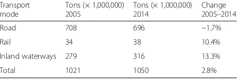
The basis of the modal shift presented in the previous section is a change in the quantities transported by each individual transport mode. Table 5 shows the direction and the size of these changes.
The observed change is negative for road and positive for rail and inland waterways. Of interest is discovering what the possible causes are for these changes. To this end we apply a shift-share analysis to decompose the changes into several components.
The shift-share method [9] derives from the field of re-gional economics, where it is often used to decompose the regional growth of jobs or productivity (see Nazara and Hewings [29], for example). In our study the vari-able of interest is the growth in the number of tons transported, and the three transport modes - road, rail and inland waterways - are the objects to which the method is applied. Notteboom and Coeck [33] have taken a similar approach in examining intermodal com-petition in Belgian inland transportation. Freight trans-port data from 1980 to 1991 and a shift-share analysis were used to position the main inland transport modes -road, rail, and inland waterways - and assess and par-tially explain the changing patterns in intermodal competition.
Table 4Size of the distance markets in tons (including those in containers)
Distance class
Absolute (tons × 1.000.000) Relative
2005 2014 2005 2014
0–50 km 315 317 30.8% 30.2%
50–100 km 131 182 12.9% 17.3%
100–300 km 377 360 37.0% 34.3%
300–500 km 80 82 7.8% 7.8%
> 500 km 118 109 11.5% 10.4%
All 1021 1050 100.0% 100.0%
Source: Statistics Netherlands and calculations by KiM
Table 5Change in transported number of tons per transport mode
Transport mode
Tons (× 1,000,000) 2005
Tons (× 1,000,000) 2014
Change 2005–2014
Road 708 696 −1.7%
Rail 34 38 10.4%
Inland waterways 279 316 13.3%
Total 1021 1050 2.8%
Source: Statistics Netherlands and calculations by KiM
The shift-share analysis decomposes absolute growth in freight transport between two years into a trans-port market effect, a cargo market effect, and a com-petition effect for each transport mode. The transport market effect is equal to the expected growth of each transport mode, as if it had developed like the total transport sector. The cargo market effect results from the specialization of a transport mode in growing and shrinking cargo markets. Finally, the competition ef-fect is the result of an increase or decrease of a transport mode’s market share in the cargo markets where it is active. The competition effect is an indica-tor for transport mode’s competitiveness. The decom-position of each transport mode’s total growth can now be presented in eq. 1. We refer to Table 6 for a description of the symbols.
Qtþli −Qti ¼TMiþCMiþCi ð1Þ
Qtiþl−Qti is total growth in tons during the period under analysis. The three components are calculated as follows:
TMi¼Qtið ÞG ð2Þ
CMi¼QtiðGi−GÞ ð3Þ
Ci¼Qti gi−Gi
ð4Þ
In order to conduct a shift-share analysis for each mode, a summation overiis needed, as shown in eq.5.
X
i Q tþl i −Qti
¼XiTMiþ
X
iCMiþ
X
iCi ð5Þ
In our application of eq. 5, t= 2005 and t + l= 2014. The results of the shift-share analysis is pre-sented in Fig. 2. The horizontal axis shows the vari-ous components’contributions to the total growth.
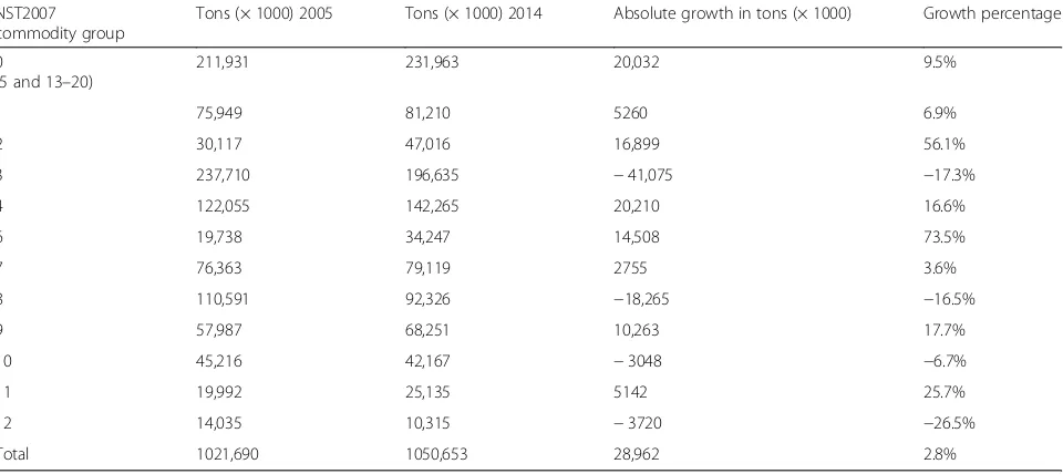
The transport market effect is, logically, equal for all three modes. This effect is represented by the blue bars in Fig. 2. The decomposition reveals that the overall positive growth for inland waterways was the result of a positive transport market effect, nega-tive cargo market effect and strong posinega-tive competi-tion effect. The negative cargo market effect resulted from a specialization in shrinking commodity mar-kets 3 and 8 in the Standard Goods Classification for Transport Statistics 2007 (NST2007). Table 7 shows that these commodity markets experienced the largest absolute decrease. The positive competi-tion effect was mainly due to gains in market share in cargo markets 3, 7, and 8. In total, the inland wa-terways’ competition effect was positive in eight of the eleven cargo markets, which implies that inland waterways possess unobserved factors that render this mode more competitive. These unobserved fac-tors can be highly diverse. CCNR [6] notes that “the waterways still have spare capacity”, and this was ap-parent in 2012 when the inland waterways were able to compensate for the lost production of two oil re-fineries. Inland waterways may therefore be better suited than other modes to handle increases in de-mand for liquid bulk transport and consequently capturing a larger part of the pie. Another possible cause could be improvements to waterway infra-structure. In 2013 a new lock was opened in the Mittelweser waterway in Germany [41]. Desk re-search focusing on specific transport markets can thus identify likely causes for the competition effect. Rail’s positive transport market effect was accompan-ied by a strong positive cargo market effect. In examining the data it appears that rail is specialized in growing cargo markets 2, and a ‘residual’ group ‘0’ consisting of cargo markets 5 and 13–20.5
Fur-ther, rail benefitted from a small positive competition-effect, which was mainly the result of its strong gain in cargo market 2. Road’s negative
overall growth was caused by a negative
competition-effect, which was larger than the sum of the positive transport market effect and cargo ket effect. Road especially lost freight in cargo mar-kets 3, 7, and 8.6
Table 6Explanation of the symbols in the equations (1)–(6)a
Symbol Description
Q quantity, number of tons transported
TM transport market effect, tons
CM cargo market effect, tons
C competition effect, tons
t year
l length of period under analysis, in years
i cargo type
G growth percentage of the total transport market
Gi general growth percentage of cargo typei
gi mode specific growth percentage of cargo typei
ΔCO2 change in CO2 emission
Ad average distance
Ef emission factor
d distance market
m mode before shift
n mode after shift
a
3 CO2emission analysis tool
In addition to the total transport market, shift-share ana-lysis can also be applied to the individual distance mar-kets, as considered in Section 2.2. This offers the opportunity to identify differences in cargo market ef-fects and competition efef-fects between the various dis-tance markets. We have seen in Section 2.3 that the competition effect of inland waterways and the cargo type effect for rail are positive in the total transport mar-ket. However, it is likely that the size of the effect varies among the distance markets. We have therefore repeated the shift-share analysis for all five distance markets. In examining the results in Appendix 2, we observe much more pronounced changes in transported quantities
between 2005 and 2014, as compared to the results for the total market in Fig.2. The amounts transported dou-bled (IWW, 300–500 km) or more than halved (rail, 50– 100 km) for several combinations of distance market and transport mode. Consequently, the three components resulting from the shift-share analysis also garner more extreme values.
The shift-share components offer useful material for a tool that is capable of assessing a modal shift’s contribu-tion to CO2 emission reduction. This tool is presented as a framework in Fig. 3. The framework’s horizontal axis represents the value of the competition effect and the vertical axis the value of the cargo market effect.7 Next, balls are used in the framework to denote all
Fig. 2Result shift-share analysis on growth tons transported between 2005 and 2014 to, from and within the Netherlands. Source: Statistics Netherlands, calculations by KiM. Note: IWW = Inland waterways
Table 7Development of cargo markets between 2005 and 2014
NST2007 commodity group
Tons (× 1000) 2005 Tons (× 1000) 2014 Absolute growth in tons (× 1000) Growth percentage
0
(5 and 13–20)
211,931 231,963 20,032 9.5%
1 75,949 81,210 5260 6.9%
2 30,117 47,016 16,899 56.1%
3 237,710 196,635 −41,075 −17.3%
4 122,055 142,265 20,210 16.6%
6 19,738 34,247 14,508 73.5%
7 76,363 79,119 2755 3.6%
8 110,591 92,326 −18,265 −16.5%
9 57,987 68,251 10,263 17.7%
10 45,216 42,167 −3048 −6.7%
11 19,992 25,135 5142 25.7%
12 14,035 10,315 −3720 −26.5%
Total 1021,690 1050,653 28,962 2.8%
combinations of transport mode, except for road, and distance market.8The color of a ball indicates whether a transport mode is responsible for a decrease (pink) or increase (red) in CO2 emissions due to a modal shift. The size of the balls depends on the distance market, the size of the modal shift due to the CM-effect and C-effect in tons, and the emission factors of the trans-port modes. Consequently, the size of a ball is an indica-tion of the size of the CO2impact resulting from a shift from one transport mode to another in a particular dis-tance market.
In order to estimate the color and size of the balls, the shift in the number of tons transported from one mode to another in each distance market must be
translated into ton-kilometers. Because ton-kilometers are missing in our dataset, we have assumed that ac-tual distances for road transport are uniformly distrib-uted around the mean distance in each distance market. For rail and inland waterways we assume a detour factor of 1.2 compared to road, because the rail and inland waterway networks have a lower dens-ity than the road network. See Table 8 for the average distances. We acknowledge that the above-mentioned assumption is quite strong; however, because our pa-per’s stated aim is to illustrate the use of the tool, we consider this simplification acceptable at this time. We do acknowledge however that it would be better to work with ton-kilometre data.
Fig. 3Positioning of rail and inland waterways based on the shift-share components and according to their contribution to CO2reduction. This framework was inspired by PBL [35]. Note: the ball for IWW 0–50 km is very small and located behind the ball for‘Rail > 500 km’.
Table 8Assumed average distances in the distance markets
Distance market Average distance road Average distance rail and IWW
0–50 25 30
50–100 75 90
100–300 200 240
300–500 400 480
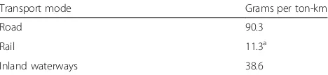
In a next step the shift in CO2 emission is calcu-lated for each distance market as follows: the num-ber of tons shifted due to the joint CM- and C-effect is multiplied by the distance and emission factor of the transport modes before and after the shift. Finally, the mode’s emissions after the shift are subtracted from the mode’s emissions prior to the shift. See Eq. 6 for the mathematical formulation. The emission factors for 2014 are shown in Table 9. These factors are specifically applicable to the Dutch freight transport situation in 2014.
ΔCO2d;m;n¼ Qd;mAdd;mEfm
− Qd;nAdd;nEfn
ð6Þ
In Equation 6 ΔCO2d, m, n is the change in CO2 emission in distance market d due to a shift from mode m to mode n. For an explanation of all symbols we refer to Table 6. By means of Equation 6 the size and color of every ball in Fig. 3 is determined. Thus, the red ball denoting rail in the 300–500 km distance market results from the fact that in this market rail has lost tons to inland waterways. Because inland wa-terways’ CO2 emission factor is higher than for rail, this shift results in increases in CO2 emissions and hence a red ball. Despite the fact that 300–500 km is quite far, the ball’s size is relatively small; this is due to the fact that the number of tons shifted from rail to inland waterways is limited. Although we per-formed several sensitivity analyses by varying the average distances, this does not alter the picture in Fig. 3 very much, as the size of the balls changes only slightly.
We now turn to the interpretation of the quad-rants in the framework. The quadquad-rants are based on
the values of the CM-component and the
C-component of the shift-share analysis. The balls located in the upper right quadrant are called ‘Obvi-ous CO2 winners’; they deserve this name because these balls depict transport modes that have in-creased their market share and are specialized in cargo markets that have above-average growth rates. This is an ideal situation from a CO2 reduction per-spective for two reasons: these modes are active in
the ‘right’ cargo markets, and they are competitive,
offering a good starting position for attracting more cargo in future. The balls in the lower right quad-rant are called ‘Potential CO2 winners’, as these modes are competitive but specialized in the ‘wrong’ cargo markets, i.e. those with below-average growth. Consequently, although these modes already possess factors that make them competitive, it would be de-sirable for these cargo markets to be reorientated, so that they become more involved in the above-aver-age growth markets. Should they succeed, these balls will shift upwards and become ‘Obvious CO2 win-ners’. The balls in the lower left quadrant are called
‘Obvious CO2 losers’, as they have lost tons due to a
negative competition effect and their specialization in the wrong markets. The ‘Masked CO2 losers’, sit-uated in the upper left quadrant, find themselves in a dangerous position; their lack of competitiveness is masked by the fact that they have experienced (modest) growth in the number of tons transported because they are active in above-average growing cargo markets. However, they run the risk of ending up in the lower left ‘Obvious CO2 losers’ quadrant should these cargo markets experience a decline in future.
A first observation from Fig. 3 is that inland wa-terways has experienced a positive competition effect between 2005 and 2014 in all the distance markets. This was not the case for rail, but given the size of rail’s balls on the right side of the y-axis, rail was responsible for considerable CO2 reductions in both the longest distance market of more than 500 km and the medium distance market of 100–300 km. The balls in the ‘Obvious CO2 winners’ quadrant imply that in five out of ten distance markets rail and inland waterways are performing well in terms of competitiveness and specializing in the ‘right’ markets. Moreover, these five balls are also relatively large, implying that in terms of ton-kilometers the shift to rail and inland waterways was accomplished in the more important markets and that the tons were acquired from a mode with a higher CO2 emis-sion coefficient. The five remaining balls are located in the other quadrants, which means that rail and inland waterways are doing less well in those five markets. However, because these markets are smaller in size (in terms of ton-kilometers), the increase in CO2 emissions due to a modal shift is relatively small.9
A point of concern from a CO2 perspective is rail’s performance in the 300–500 km distance market. Rail is active in growing cargo markets within this distance market yet simultaneously has lost market share. A closer look at the data reveals that it is the Table 9CO2emission factors for 2014
Transport mode Grams per ton-km
Road 90.3
Rail 11.3a
Inland waterways 38.6
Source: KiM [20], CE Delft [7] a
fast-growing NST2007 cargo market 2 that is virtu-ally solely responsible for rail’s position in the 300– 500 km distance market. From the perspective of the transition in the energy sector and transition to-wards a circular economy, it is dangerous for rail to depend to a large extent on this cargo market. Should this cargo market shrink, rail will lose more tons than inland waterways and road (modes with higher CO2 emission factors), because rail specializes in this cargo market and will thus run the risk of moving to the ‘Obvious CO2 losers’ quadrant.
Another interesting ball is that for inland water-ways in 300–500 km distance market, where it ap-pears that NST2007 cargo markets 2 and 7 are the drivers of growth in the number of tons trans-ported. Like cargo market 2, cargo market 7 is a bulk market that is likely to be affected by the men-tioned transitions. Nevertheless, inland waterways can rely on its competitiveness in cargo market 7. Inland waterways gained market share in all cargo markets within the 300–500 km distance market, but especially in NST2007 cargo markets 0, which is the
‘residual’ group consisting of commodity groups 5
and 13–20, 2, and 10. This means that inland water-ways is strong in both the bulk and containers mar-kets, which is a good starting point for future CO2 emission reductions in this distance market.
4 Discussion
The presented framework visualizes in a glance how freight transport modes perform from a CO2 emis-sions perspective in a modal shift context. The com-bination of the size and the color of the balls immediately expresses whether, and to what extent, the modal shifts have resulted in reduced CO2 emis-sions. Additionally, the position of the balls in the framework’s quadrants express whether a transport mode is likely to contribute to the decarbonization of freight transport in future. A shift based on im-provements to a transport mode’s competitiveness is more likely to last in future than a shift based on that transport mode’s overrepresentation in above-average growing markets. In the latter case, the transport mode’s position in the framework is highly subject to the volatility of cargo markets. A transport mode’s position is more stable if it is mainly based on its competitiveness, because such competiveness will mute any possible impact from future declines of the cargo markets in which it is overrepresented..
On the basis of the framework, policy makers in the freight transport field are better able to steer their modal shift policies: they can see in which
markets inland waterways and rail perform well in terms of CO2 emission reductions due to a modal shift, and then strive to determine what the factors for success were. Conversely, they can also see where inland waterways and rail have underper-formed. The question to then be answered is how good positions for rail and inland waterways can be guaranteed in future and how less advantageous po-sitions improved. Studying the data that feed the framework in greater detail can reveal which are the most important cargo markets in terms of size, if these markets are growing or shrinking, and how competitive a transport mode is in these markets. Combining this information with expected develop-ments, such as the circular economy, ongoing energy transitions and innovations in the transport sector, can help shape successful policies aimed at the decarbonization of freight transport. Unfortunately, the tool does not elucidate the factors that lie be-hind the competition effect. Possible factors could be identified by means of desk-and field research of the specific transport markets though.
Because the tool does not reveal the reasons for being competitive ex-post, we do not know which policy interventions worked and did not work. Research methods, including those cited in Table 2, cannot reveal this either, but they can be used for ex-ante analysis and thus valuable for shaping future policies. As proposed by Marcucci et al. [26] and le Pira et al. [36], integrated discrete choice and agent-based modeling could be useful additional as-sets. The starting point for their modeling approach is that a good policy is one that provides a package of measures integrating the interests of the diverse stakeholders, which, for inland freight transport, are shippers, carriers, receivers, governments, et al.. The integrated modeling approach takes into account stakeholders’ heterogeneous preferences and simu-lates their interactive behavior in a consensus build-ing process, providbuild-ing useful suggestions for policy makers about the potential acceptability of a set of policies to be eventually discussed with stakeholders. Although these studies apply to an urban context, their approach might also be feasible on the larger spatial scale of a country or the EU.
the tool – has low data requirements and also com-puting complexity is low.
The main drawback of how the tool is applied in this paper is that data on tons was combined with assumed average distances. Hence, a key improve-ment would be to directly use ton-kilometers data instead of ‘derived’ ton-kilometers data. If for ex-ample such data were available on the EU Member State level, comparisons between countries would be possible.10 However, because the stated aim of this paper is to illustrate and explain the tool and its us-ability, the use of derived ton-kilometre data is deemed to be but a minor drawback.
5 Conclusion
We conclude that for freight transport with an origin, destination or both in the Netherlands, a modal shift from road (−3,0 percentage points), to rail (+ 0,2 per-centage points), and to inland waterways (+ 2,8 percent-age points) occurred in the period 2005–2014. No transported freight was shifted in the less than 100 km distance market. This implies that the shift for the total market wholly occurred in the more than 100 km dis-tance market. A shift-share analysis, decomposing growth in the number of tons transported by each mode, for the total transport market reveals that the modal shift mainly results from rail being specialized in the above-average growing cargo markets and from inland waterways becoming more competitive between 2005 and 2014.
The core of this research paper is however the presentation of a tool that can be used to assess how a freight modal shift contributes to CO2 emis-sion reductions. This meets the need for research into methods to address problems in the area of intermodal transport. One of these problems is that in freight transport the shift to more sustainable modes has been very modest in the past 10 to 15 years. This problem can be addressed by our tool. The assessment tool is based on the shift-share method, which is well known in the field of re-gional economics. The tool shows how rail and in-land waterways have performed in terms of CO2 emissions reduction, while taking into account the transport modes’ competitiveness and the develop-ment of the cargo markets in which they are active. The tool thus provides policy makers with valuable information about the background to changes in CO2 emission due to freight modal shifts in past years. This information can be used as a starting point for devising future freight transport policies aimed at attracting more cargo by rail and inland waterways.
6 Endnotes 1
To increase reading convenience, we would like to mention that a list of abbreviations used in this paper can be found between the conclusions and the references.
2
In Nocera and Cavallaro [31], CO2 emissions from construction are taken into account.
3
The mode shares in 2005 were 69.3% for road, 3.4% for rail, and 27.3% for inland waterways.
4
The cargo type classification we use is based on the 2007 standard goods classification for transport statis-tics, in short the NST2007 commodity classification of the European Commission [10]. The classification, with a description of the numerical cargo markets, can be found in Appendix1.
5
For analytical reasons the commodity groups 5 and 13–20 had to be aggregated into one so-called‘residual group’. This is group number 0.
6
Note that these are exactly the markets where inland waterways gained market share, which makes sense, as not all transport modes can gain market share at the same time in one cargo market. Where one mode gains market share, one or two other modes will lose.
7
To describe this as an analogy with a pie: a posi-tive value on the vertical axis implies that the pies (cargo markets) in which a transport mode has a relatively large share have grown between 2005 and 2014. A high positive value on the horizontal axis means that a transport mode has captured a larger part of the pies between 2005 and 2014.
8
Balls for road are not shown because the aim of the framework is to visualise shifts to and from the least emitting transport modes - rail and inland waterways.
9
Considering that rail has the lowest CO2 emission factor, as shown in Table 9, note that it would be ideal from a CO2perspective to have all the rail balls located in the upper right quadrant, and the IWW balls posi-tioned to the left and below the rail balls.
10
Appendix 1
Table 10NST2007 cargo type classification
Division Description
01 Products of agriculture, hunting, and forestry; fish and other fishing products
02 Coal and lignite; crude petroleum and natural gas
03 Metal ores and other mining and quarrying products; peat; uranium and thorium
04 Food products, beverages and tobacco
05 Textiles and textile products; leather and leather products
06 Wood and products of wood and cork (except furniture); articles of straw and plaiting materials; pulp, paper and paper products; printed matter and recorded media
07 Coke and refined petroleum products
08 Chemicals, chemical products, and man-made fibres; rubber and plastic products; nuclear fuel
09 Other non-metallic mineral products
10 Basic metals; fabricated metal products, except machinery and equipment
11 Machinery and equipment n.e.c.; office machinery and computers; electrical machinery and apparatus n.e.c.; radio, television and communication equipment and apparatus; medical, precision and optical instruments; watches and clocks
12 Transport equipment
13 Furniture; other manufactured goods n.e.c.
14 Secondary raw materials; municipal wastes and other wastes
15 Mail, parcels
16 Equipment and material utilised in the transport of goods
17 Goods moved in the course of household and office removals; baggage transported separately from passengers; motor vehicles being moved for repair; other non-market goods n.e.c.
18 Grouped goods: a mixture of types of goods which are transported together
19 Unidentifiable goods: goods which for any reason cannot be identified and therefore cannot be assigned to groups 01–16.
20 Other goods n.e.c.
Abbreviations
CCNR:Central Commission for Navigation on the Rhine; CGE model: Computable General Equilibrium model; CO2: Carbon dioxide; COP21: 21st Conference Of Parties; EU: European Union; EU28: The current 28 members of the European Union; GHG: Green House Gas;
GIS: Geographical Information System; IWW: Inland Waterways; LCA: Life Cycle Analysis; NST2007: Standard goods classification for transport statistics 2007; NUTS: Nomenclature of Territorial Units for Statistics; OD matrix: Origin-Destination matrix; RP: Revealed Preference; SP: Stated Preference; SSS: Short-Sea Shipping
Acknowledgements
The authors would like to thank two anonymous referees and the participants of the NECTAR Cluster meeting on‘The future of freight transport’, held on March 8-9, 2018, in Venice Italy, for their valuable comments.
Funding
For this study no specific funds were received. KiM Netherlands Institute for Transport Policy Analysis has an annual budget from which all research is financed.
Availability of data and materials
The data that support the findings of this study are available from Statistics Netherlands but restrictions apply to the availability of these data, and so are not publicly available. Data are however available from the authors upon reasonable request and with permission of Statistics Netherlands.
Authors’contributions
OJ performed the shift-share analyses, invented the framework and did most of the writing. JF did the acquisition of the data from Statistics Netherlands, made an intellectual contribution to the analyses and assisted in writing the article. JV made an intellectual contribution to the analyses and assisted in writing the article. All authors read and approved the final manuscript.
Competing interests
The authors declare that they have no competing interests.
Publisher’s Note
Springer Nature remains neutral with regard to jurisdictional claims in published maps and institutional affiliations.
Received: 13 June 2018 Accepted: 3 January 2019
References
1. Arencibia, A. I., Feo-Valero, M., Garcia-Menendez, L., & Roman, C. (2015). Modelling choice for freight transport using advanced choice experiments.
Transp Res A.https://doi.org/10.1016/j.tra.2015.03.027.
2. Asuncion J, Rendall S, Murray R, Krumdieck S (2012) New Zealand intermodal freight network and the potential for mode shifting. University of Canterbury, Christchurch New Zealand.
3. de Bok M, Wesseling B, Kiel J, Miete O, Francke J (2017) An exploration of freight transport forecasts for the Netherlands with Basgoed. Paper which follows for a research project for the Dutch Ministry of Infrastructure and Water Management.
4. Bontekoning, Y. M., Macharis, C., & Trip, J. J. (2004). Is a new applied research field emerging?–A review of intermodal rail-truck freight transport literature.Transp Res A.https://doi.org/10.1016/j.tra.2003.06.001.
5. Buhler, G., & Jochem, P. (2008).CO2Emission Reduction in Freight Transports. How to Stimulate Environmental Friendly Behaviour?Discussion Paper No. 08–066. Centre for European Economic Research.
6. CCNR. (2014).Inland navigation in Europe, market observation 2014. Strasbourg: Central Commission for the Navigation of the Rhine. 7. Delft, C. E. (2017).STREAM Freight Transport 2016 (in Dutch), Emissions of freight
transport modes–Version 2, Publication code: 17.4H29.10. Delft: CE Delft.
Appendix 2
Table 11Shift-share results for the five distance markets
Tons 2005 Tons 2014 % change TM-effect CM-effect C-effect
Distance market 0–50 km
Road 291,240,398 293,509,387 0.8% 0.6% 0.8% −0.6%
Rail 1,042,875 424,153 −59.3% 0.6% 58.3% −118.2%
IWW 22,666,423 22,876,538 0.9% 0.6% −12.7% 13.0%
Distance market 50–100 km
Road 90,441,652 131,711,026 45.6% 38.3% 8.8% −1.4%
Rail 1,226,300 315,033 −74.3% 38.3% −4.9% −107.7%
IWW 39,764,105 49,919,460 25.5% 38.3% −20.2% 7.4%
Distance market 100–300 km
Road 208,860,765 188,594,615 −9.7% −4.5% −0.7% −4.5%
Rail 9,531,849 13,940,457 46.3% −4.5% 4.9% 45.9%
IWW 159,125,896 157,924,527 −0.8% −4.5% 0.7% 3.1%
Distance market 300–500 km
Road 53,690,766 31,651,994 −41.0% 2.6% −18.5% −25.1%
Rail 4,287,383 2,585,584 −39.7% 2.6% 74.2% −116.5%
IWW 21,734,196 47,518,322 118.6% 2.6% 31.0% 85.1%
Distance market > 500 km
Road 63,798,975 50,765,389 −20.4% −7.1% −2.9% −10.4%
Rail 18,163,737 20,628,259 13.6% −7.1% 1.6% 19.1%
8. Cloodt, H. (2009).Modal Split of freight transport according to the territoriality principle (2008–2009), statistics in focus, 13/2012. Eurostat.
9. Dunn, E. S. (1960). A statistical and analytical technique for regional analysis.
Papers of the Regional Science Association, 6, 97–112.
10. European Commission. (2007).Commission regulation (EC) no 1304/2007. Brussels: 7 November 2007.
11. Eurostat (2018) Eurostat statistics explained: Freight transport statistics– Modal split. Website:https://ec.europa.eu/eurostat/statistics-explained/index. php/Freight_transport_statistics_-_modal_split#Modal_split_in_the_EU
12. Fraunhofer (2018) Energy Charts, website visited 17/09/2018:https://www. energy-charts.de/osm.htm.
13. Gössling, S., Cohen, S. A., & Hares, A. (2016). Inside the black box: EU policy officers’perspecitves on transport and climate change mitigation.J Transp Geogr.https://doi.org/10.1016/j.jtrangeo.2016.10.002.
14. Islam, D. M. Z., Jackson, R., Zunder, T. H., & Burgess, A. (2015). Assessing the impact of the 2011 EU transport white paper–A rail freight demand forecast up to 2050 for the EU27.Eur Transp Res Rev.https://doi.org/10. 1007/s12544-015-0171-7.
15. Islam, D. M. Z., & Zunder, T. H. (2018). Experiences of rail intermodal freight transport for low density high value (LDHV) goods in Europe.Eur Transp Res Rev.https://doi.org/10.1186/s12544-018-0295-7.
16. de Jong, G., Vierth, I., Tavasszy, L., & Ben-Akiva, M. (2013). Recent developments in national and international freight transport models within Europe.Transportation.https://doi.org/10.1007/s11116-012-9422-9. 17. Jonkeren, O., Jourquin, B., & Rietveld, P. (2011). Modal-split effects of climate
change: The effect of low water levels on the competitive position of inland waterway transport in the river Rhine area.Transp Res A.https://doi.org/10. 1016/j.tra.2009.01.004.
18. Jonkeren, O., Francke, J., & Visser, J. (2017).Ontwikkeling van de modal split in het goederenvervoer, KiM Netherlands Institute for Transport Policy Analysis, KIM-17-A06. The Hague.
19. Kaack, L. H., Vaishnav, P., Morgan, M. G., Azevedo, I. L., & Rai, S. (2018). Decarbonizing intraregional freight systems with a focus on modal shift.
Environ Res Lett.https://doi.org/10.1088/1748-9326/aad56c.
20. KiM. (2016).Mobility report 2016 (in Dutch), KiM Netherlands Institute for Transport Policy Analysis, KiM-16-R01. The Hague.
21. Kim, N.S., & van Wee B. (2008) Assessment of CO2emissions for intermodal freight transport systems and truck-only systems: A case study of the western-eastern Europe corridor. Paper submitted for presentation at NECTAR Cluster Meeting 2008.
22. Kim, N.S., & van Wee, B. (2009). Assessment of CO2emissions for truck-only and rail-based intermodal freight systems in Europe.Transp Plan Technol.
https://doi.org/10.1080/03081060903119584.
23. Macharis, C., & Bontekoning, Y. M. (2004). Opportunities for OR in intermodal freight transport research: A review.Eur J Oper Res.https://doi.org/10.1016/ S0377-2217(03)00161-9.
24. Macharis C, van Hoeck E, Pekin E, van Lier T (2010) A decision analysis framework for intermodal transport: Comparing fuel price increases and the internalisation of external costs. Transp Res A doi:https://doi.org/10.1016/j. tra.2010.04.006.
25. Marcucci, E., & Gatta, V. (2016). How good are retailers in predicting transport providers’preferences for urban freight policies? ,,, and vice versa?
Transp Res Proc.https://doi.org/10.1016/j.trpro.2016.02.058.
26. Marcucci, E., le Pira, M., Gatta, V., Inturri, G., Ignaccolo, M., & Pluchino, A. (2017). Simulating participatory urban freight transport policy-making: Accounting for heterogeneous stakeholders’preferences and interaction effects.Transp Res E.https://doi.org/10.1016/j.tre.2017.04.006.
27. Meers, D., & Macharis, C. (2015). Priorization in modal shift: Determining a region’s most suitable freight flows.Eur Transp Res Rev.https://doi.org/10. 1007/s12544-015-0172-6.
28. Mostert, M., Caris, A., & Limbourg, S. (2017). Road and intermodal transport performance: The impact of operational costs and air pollution external costs.Res Transp Bus Manag.https://doi.org/10.1016/j.rtbm.2017.02.004. 29. Nazara, S., & Hewings, G. J. D. (2004). Spatial structure and taxonomy of decomposition in shift-share analysis.Growth Chang, 35(4), 476–490. 30. Nelldal, B.-L., & Andersson, E. (2012). Mode shift as a measure to reduce
greenhouse gas emissions.Procedia Soc Behav Sci.https://doi.org/10.1016/j. sbspro.2012.06.1285.
31. Nocera, S., & Cavallaro, F. (2014). A methodological framework for the economic evaluation of CO2emissions from transport.J Adv Transp.https://
doi.org/10.1002/atr.1249.
32. Nocera, S., & Cavallaro, F. (2016). Economic valuation of well-to-wheel CO2 emissions from freight transport along the main transalpine corridors.
Transp Res D.https://doi.org/10.1016/j.trd.2016.06.004.
33. Notteboom, T., & Coeck, C. (1994). Strategic positioning within the Belgian freight transport market (in Dutch).Tijdschrift Vervoerswetenschap, 2, 85–110. 34. Ortuzar J de, D., & Willumsen, L. G. (2011).Modelling Transport. Chichester
(UK): John Wiley & Sons.
35. PBL, (2017) Winners and losers in Regional Economic Competition, PBL Netherlands Environmental Assessment Agency, interactive webtool:http:// themasites.pbl.nl/winnaars-verliezers-regionale-concurrentie/#/front?region=R175. 36. le Pira, M., Marcucci, E., Gatta, V., Ignaccolo, M., Inturri, G., & Pluchino, A.
(2017). Towards a decision-support procedure to foster stakeholder involvement and acceptability of urban freight transport policies.Eur Transp Res Rev.https://doi.org/10.1007/s12544-017-0268-2.
37. Regmi, M. B., & Hanaoka, S. (2013). Assessment of odal shift and emissions along a freight transport corridor between Laos and Thailand.Int J Sustain Transp.https://doi.org/10.1080/15568318.2012.754972.
38. Ruesch, M. (2001).Potentials for modal shift in freight transport(Paper presented at the 1st Swiss transport research conference). Monte Verita / Ascona: March 1–3, 2001.
39. Schwierz, S. (2017).The role of transport sector in CO2 reduction in Poland, E3S Web of Conferences(p. 14).https://doi.org/10.1051/e3sconf/ 20171401010.
40. Tavasszy L, van Meieren J (2011) Modal Shift Target for Freight Transport Above 300 km: An Assessment. Discussion paper 17th ACEA SAG Meeting. 41. Totaaltrans (2018) Website visited 01/10/2018:http://www.totaaltrans.nl/
nieuwe-sluis-dorverden-open-voor-grote-schepen/
42. Tsamboulas, D., Vrenken, H., & Lekka, A.-M. (2007). Assessment of a transport policy potential for intermodal mode shift on a European scale.Transp Res A.https://doi.org/10.1016/j.tra.2006.12.003.
43. Zhang, M., & Pel, A. J. (2016). Synchromodal hinterland freight transport: Model study for the port of Rotterdam.J Transp Geogr.https://doi.org/10. 1016/j.jtrangeo.2016.02.007.